Aging processes in systems with anomalous slow dynamics

Abstract

Recently, different numerical studies of coarsening in disordered systems have shown the existence of a crossover from an initial, transient, power-law domain growth to a slower, presumably logarithmic, growth. However, due to the very slow dynamics and the long lasting transient regime, one is usually not able to fully enter the asymptotic regime when investigating the relaxation of these systems toward equilibrium. We here study two simple driven systems, the one-dimensional $ABC$ model and a related domain model with simplified dynamics, that are known to exhibit anomalous slow relaxation where the asymptotic logarithmic growth regime is readily accessible. Studying two-times correlation and response functions, we focus on aging processes and dynamical scaling during logarithmic growth. Using the time-dependent growth length as the scaling variable, a simple aging picture emerges that is expected to also prevail in the asymptotic regime of disordered ferromagnets and spin glasses.

I Introduction

Recent years have seen remarkable progress in our understanding of physical aging in non-disordered systems with slow, i.e. glassy-like, dynamics (see book10 for a recent comprehensive overview). In many systems, ranging from ferromagnets undergoing phase-ordering Bra94 to reaction-diffusion systems Hen07 , a single dynamical length $L(t)$, that grows as a power-law of time $t$, governs the dynamics out of equilibrium. In the aging or dynamical scaling regime these systems are best characterized by two-times quantities, like dynamical correlation and response functions, that transform in a specific way under a dynamical scale transformation Cug03 . The resulting dynamical scaling functions and the associated non-equilibrium exponents are often found to be universal and to depend only on some global features of the system under investigation.

However, growth laws can be much more complicated, as discussed recently in disordered ferromagnets quenched below their critical temperature. Thus, convincing evidence for a dynamic crossover between a transient regime, characterized by a power-law growth with an effective dynamical exponent that depends on the disorder, and the asymptotic regime, where the growth is logarithmic in time, has been found in recent studies of the dynamics of elastic lines in a random potential Kol05 ; Noh09 ; Igu09 ; Mon09 as well as in numerical simulations of disordered Ising models Rao93 ; Aro08 ; Par10 ; Cor11 ; Cor11a ; Cor12 ; Par12 . These indications are compatible with the classical (droplet) theory of activated dynamics that, under the assumption of energy barriers growing as a power of $L$, predicts a slow logarithmic increase Hus85 of this length:

$$L\sim(\ln t)^{1/\psi},$$ (1)

with the barrier exponent $\psi>0$. Whereas in some of the studies on disordered Ising models aging phenomena in the crossover regime were investigated Aro08 ; Par10 ; Cor11 ; Cor11a ; Cor12 ; Par12 , none of these recent numerical studies was able to enter so deeply into the asymptotic regime that no corrections to the logarithmic growth law were detectable any more. Therefore a systematic study of aging processes in this regime with pure logarithmic growth has not yet been done.

In this paper we study two one-dimensional models that exhibit anomalous slow dynamics and that are known to display coarsening where the length of the domains increases logarithmically with time Eva02 . Even though these models are in no way related to disordered ferromagnets and spin glasses, their studies should allow us to gain a better understanding of the generic properties of an aging system with a logarithmic growth law.

The models discussed in the following are the so-called $ABC$ model Eva98a , a driven diffusive system composed of three different types of particles that swap places asymmetrically, and a related domain model Eva98b whose simplified dynamics is supposed to capture the dynamics of the $ABC$ model at the later stages of the coarsening process. The $ABC$ model has recently yielded a flurry of interesting studies Cli03 ; Bod08 ; Ayy09 ; Led10a ; Led10b ; Bar11a ; Ber11 ; Bar11b ; Ger11 ; Coh11 ; Bod11 ; Ger12 ; Coh12 ; Coh12b that helped establishing it as a paradigm for systems far from equilibrium. Not only is the $ABC$ model characterized by its anomalous slow dynamics, making it a representative for a larger class of systems with a similar coarsening process Lah97 ; Arn98 ; Lah00 ; Kaf00 ; Lip09 , it also exhibits a variety of interesting non-equilibrium phase transitions whose properties change dramatically when breaking certain conservation laws. The domain model has been proposed as a simplified version of the $ABC$ model where only movements of particles between domains of the some species are considered. This simplified dynamics accelerates the coarsening process and allows to enter the purely logarithmic growth regime faster Eva98b . In the following we use the $ABC$ model in order to investigate the onset of dynamical scaling, whereas the domain model is used to characterize aging scaling deep inside the logarithmic growth regime.

Our paper is organized as follows. In the next Section we discuss in more detail the two models that we study. Section III is devoted to the aging processes taking place in the $ABC$ model. We thereby focus on the two-times autocorrelation function where the two times are not always in the asymptotic, logarithmic scaling regime. In Section IV we characterize aging scaling in the domain model through the study of both correlation and response functions. We discuss our results in Section V.

II Models and quantities

In the $ABC$ model particles of three different species live on a one-dimensional ring Eva98a . Every lattice site is occupied by exactly one particle, which can swap places with its left and right neighbors. In the symmetric case, where all exchanges happen with the same rate, every particle undergoes a random walk, and nothing interesting takes place. However, this changes dramatically as soon as one introduces a bias which makes the particles diffuse asymmetrically around the ring. This is achieved by randomly selecting a pair of neighboring sites and updating them using the following rates:

$$AB\overset{q}{\underset{1}{\rightleftarrows}}BA$$

$$BC\overset{q}{\underset{1}{\rightleftarrows}}CB$$

$$CA\overset{q}{\underset{1}{\rightleftarrows}}AC$$ (2)

with $q<1$. As a result of these rules, phase separation takes place in such a way that the ordered domains arrange themselves in repetitions of the sequence $ABC$, where $A$ indicates a domain of $A$ particles, followed by a domain of $B$ particles, which itself is followed by a $C$ domain. Once this arrangement has been achieved, the domains coarsen whereby the typical domain size increases logarithmically with time.

Obviously these exchanges keep constant the total number of particles of each species. We consider in our study only lattice sizes divisible by three and initially populate one third of the lattice sites by particles of each species. In that case detailed balance is fulfilled and the system evolves toward an equilibrium steady state Eva98a .

In the domain model one focuses on the later stages of the coarsening process where well-defined, compact domains have already formed. One then defines a simplified dynamics where only events are taken into account that change the sizes of two neighboring domains of the same species. For example, consider the case where two such $A$ domains are selected, called $A_{l}$ and $A_{r}$, that are separated by one $B$ and one $C$ domain, yielding the sequence $\cdots A_{l}BCA_{r}\cdots$. Calling $a_{l}$ respectively $a_{r}$ the domain size of the domain $A_{l}$ respectively $A_{r}$, these domain sizes are then modified in one of the following two ways Eva98b :

$$a_{l}\longrightarrow a_{l}-1~{}~{},~{}~{}a_{r}=a_{r}+1~{}~{}~{}\mbox{with rate}~{}q^{b}$$

$$a_{l}\longrightarrow a_{l}+1~{}~{},~{}~{}a_{r}=a_{r}-1~{}~{}~{}\mbox{with rate}~{}q^{c}$$

where $b$ respectively $c$ are the number of sites of the $B$ respectively $C$ domain separating our two $A$ domains. These rates follow from the observation that in order to go from one domain to the other an $A$ particle has to cross one of the two intermediate domains in the ‘wrong’ direction. The domain model therefore exclusively considers processes where particles successfully travel between domains of the same type, irrespective on how many jumps are needed for that transit.

Two-times quantities are well suited to study relaxation processes far from equilibrium book10 . We here briefly recall the expected behavior of such quantities, without entering into the details on how these quantities are computed for our driven diffusive systems. This will be done in the following Sections when we discuss our numerical results.

The two-times quantities usually at the center of aging studies are the autocorrelation function $C(t,s)$ and the autoresponse function $R(t,s)$. The autocorrelation function measures the extend to which configurations taken at two different times $s$ and $t>s$ are correlated. Here $s$ is the waiting time, whereas $t$ is called the observation time. The autoresponse function, on the other hand, allows us to investigate how the system reacts during the relaxation process to a instantaneous perturbation (as for many other studies, we will focus below on the time integrated response to a longer lasting perturbation which is much easier to measure). In the aging regime, where the observation and waiting times are large compared to any microscopic time scale, the single growth length $L$ dominates the properties of the system, so that the different quantities should depend on time only through this length $L$. Thus one expects the following (very general) scaling forms, using standard notation book10 :

$$C(t,s) = \left(L(s)\right)^{-b}f_{C}\left(\frac{L(t)}{L(s)}\right)$$ (3)

$$R(t,s) = \left(L(s)\right)^{-1-a}f_{R}\left(\frac{L(t)}{L(s)}\right)$$ (4)

with the scaling functions $f_{C}(y)$ and $f_{R}(y)$ and the non-equilibrium exponents $a$ and $b$. In systems undergoing coarsening one usually has $b=0$ and $a\neq 0$, but this can be different in other situations, as for example during non-equilibrium relaxation at a critical point Cal05 . In cases with an algebraic growth law $L(t)\sim t^{1/z}$, as observed in critical systems or coarsening systems without disorder, one usually uses $t/s$ as scaling variable. However, for more complicated cases with subleading contributions to the growth and/or crossover between an initial algebraic growth and the true asymptotic behavior, this approach is too simplistic and $L(t)/L(s)$ has to be used as variable in order to achieve the expected scaling Par10 ; Par12 .

III Aging in the $ABC$ model

In our simulations of the original $ABC$ model we focus on the early time regime where coarsening slowly sets in. We thereby always prepare the system in a disordered initial state with every species occupying one third of the lattice sites chosen at random. The data presented below have been obtained for rings with $N=9000$ sites. This is large enough so that no finite size effects show up for the times accessed in our simulations, as we checked by making additional runs for other system sizes. We define one time step as $N$ proposed updates. For every proposed update we select a pair of neighboring sites at random and then exchange them with the rates given in (II).

III.1 Domain growth

We start by having a look at the average domain size. Fig. 1 shows $L(t)$ for a large range of $q$ values. We note that in all cases an initial regime is observed during which domains are formed and arranged in the correct sequence, so that a $C$ domain follows a $B$ domain that follows an $A$ domain. This initial regime lasts longer for larger values of $q$ as it gets increasingly difficult to form these initial domains the closer $q$ gets to 1.

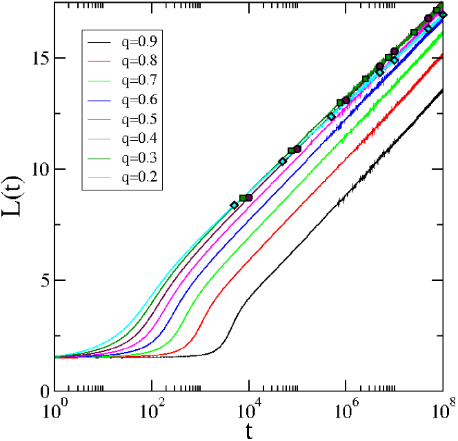
Figure 1: (Color online) Time-dependent average domain size for the $ABC$ model with various values of the rate $q$. After some initial regime, that lasts longer the larger the value of $q$, logarithmic growth sets in. The slopes in the log-linear plot increase with $q$. The data result from averaging over 600 independent runs. For small $t$ values, the curves are ordered in such a way that the largest $q$ value corresponds to the lowest curve, whereas the smallest $q$ value yields the highest curve. For larger $t$ the curves start to cross, due to difference in slopes. In order to make this crossing better visible, some selected data points are shown as symbols (circles: $q=0.4$, squares: $q=0.3$, diamonds: $q=0.2$).

Once these initial domains are formed, they then coarsen, and the system size increases logarithmically with time: $L(t)\sim\ln t$. Obviously, this is a very slow process and even after $10^{8}$ time steps the average domain size does not reach twenty lattice spacings. This coarsening proceeds faster for larger values of $q$. Indeed, the slopes in the log-linear plot decrease when decreasing $q$. Thus, in the interval between $t=10^{6}$ and $t=10^{8}$ we obtain that the slope continuously decreases from 1.05 for $q=0.9$ to 0.86 for $q=0.2$. Whereas at short times the domain size is the largest for the smallest $q$ value, we expect the order to be reversed for very long times, due to the difference in slopes. In fact, indications of this are already seen in Fig. 1, see the two curves for $q=0.2$ and $q=0.3$ that start to be below some of the curves obtained for larger $q$ values.

A closer inspection of the curves in Fig. 1 for the smallest $q$ values 0.2 and 0.3 reveals that their slopes change slightly with time. Even after $t=10^{8}$ time steps we are for these $q$ values not yet completely inside the asymptotic regime where corrections to the logarithmic growth law should be completely absent.

III.2 Autocorrelation

As mentioned in the introduction, valuable insights into relaxation far from equilibrium can be gained through the study of two-times quantities. In this subsection we discuss the autocorrelation $C(t,s)$. For our three species system we characterize lattice site $i$ by a time-dependent Potts variable $p_{i}(t)$(alternatively we could use a species dependent occupation number Afz11 ; Ahm12 ) that can take on the three different values 0, 1, or 2, depending on whether at time $t$ the site is occupied by an $A$, $B$, or $C$ particle. The autocorrelation function $C(t,s)$ is then defined as

$$C(t,s)=\left<\frac{1}{N}\sum\limits_{i=1}^{N}\delta_{p_{i}(t),p_{i}(s)}\right>-\frac{1}{3}$$ (5)

where $\delta_{\alpha,\beta}$ is the Kronecker delta. In that equation $\left<\cdots\right>$ indicates an average over both initial conditions and noise as realized through different random number sequences. We subtract from this average the value 1/3 that one has for two completely uncorrelated configurations, thus making sure that $C(t,s)$ approaches zero when t gets very large.

In our simulations we averaged over a large number of realizations, ranging from 600 for the longest waiting times to 20000 for the shortest waiting times. In all cases we let the system evolve for $t=40~{}s$ time steps where $s$ is the waiting time.

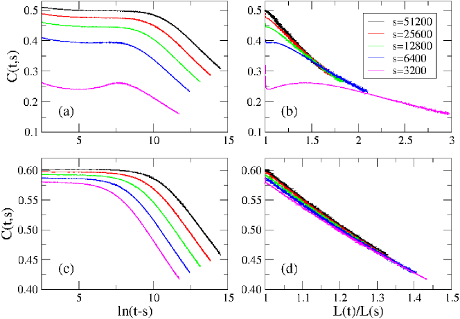
Figure 2: (Color online) Autocorrelation function for the $ABC$ model with (a,b) $q=0.9$ and (c,d) $q=0.3$. For every waiting time $s$ we compute the autocorrelation function for up to $t=40~{}s$ time steps. Plotting the autocorrelation against the scaling variable $L(t)/L(s)$, see (b) and (d), yields indications for the onset of dynamical scaling for the longest waiting times. The data result from averaging over at least 600 independent runs. The values of the autocorrelation increase with increasing waiting times.

The data shown in Fig. 2 for $q=0.9$ and $q=0.3$ are representative for all studied values of $q$. Comparing data for different waiting times reveal the expected physical aging where the two-times quantity is not simply a function of the time difference, see Fig. 2a and 2b. For $q=0.9$ the behavior for the shortest waiting time shown in Fig. 2a clearly differs from that observed for the larger waiting times. In fact, inspection of Fig. 1 reveals that $s=3200$ lies in the time regime where the initial domains are forming and where coarsening starts to set in. As a result correlations dramatically change in the system, which is revealed by the non-monotonous behavior of the autocorrelation function.

In Fig. 2b and 2d we test dynamical scaling by plotting the data as a function of $L(t)/L(s)$. Clear deviations are observed for the smaller waiting times, but these deviations get less and less important the larger $s$ gets, yielding for $q=0.3$ already a good data collapse for the largest waiting times. All this indicates that for very large $s$ we start to be in the aging scaling regime. In agreement with Fig. 1 the scaling regime is accessed more rapidly for the smaller $q$ values. We also note that even for $t/s=40$, the ratio of the corresponding lengths $L(t)/L(s)$ remains rather small. Obviously, the regime $L(t)/L(s)\gg 1$ remains out of reach in systems displaying logarithmic growth.

IV Aging in the domain model

It follows from the discussion in the previous Section that it is extremely difficult to fully enter the asymptotic growth regime for the $ABC$ model. We therefore focus in the following on the domain model with simplified dynamics that captures the essential properties of the $ABC$ model deep inside the coarsening regime while speeding up the dynamics Eva98b .

For the domain model we consider systems with $N=27000$ sites, thereby checking carefully that no finite-size effects affect our data for the times accessed in our simulations. As the dynamics assumes the existence of domains that coarsen, we prepare our system in an initial state where we have 3000 sequences of $ABC$ domains, with every domain extending over three lattice sites. We then start the system with the chosen value of $q$. During the simulations smaller domains tend to disappear as larger domains keep growing. If, say, an $A$ domain vanishes in the original $ABC$ model, this yields a sequence $ABCBCA$, which rapidly evolves into a sequence $ABCA$ as for two neighboring sites $CB$ is replaced by $BC$ with rate 1. The resulting $B$ respectively $C$ domains have then sizes that are identical to the sums of the sizes of the two $B$ respectively $C$ domains at the moment of the dismissal of the $A$ domain. In the domain model this merging is done immediately whenever a domain vanishes Eva98b . For simplicity we increase in our simulations time $t$ by one unit when the number of proposed updates is equal to the number of domains that are in the system at time $t$.

IV.1 Domain growth

In Fig. 3 we verify that we are indeed deep inside the logarithmic growth regime for all studied values of $q$. As already observed in Eva98b , the logarithmic growth sets in very rapidly when using the simplified dynamics. We note that the growth proceeds faster for larger values of $q$. This is of course in agreement with our observation in Fig. 1 that for the system with the full dynamics the prefactor in the equation (which corresponds to the slope in the log-linear plot)

$$L(t)=\gamma\ln t$$ (6)

is decreasing when $q$ decreases. In Eva98b it has been proposed that the length should grow as

$$L(t)=p\ln t/|\ln q|~{}$$ (7)

for the domain model. We indeed obtain consistently a value of $p\approx 2.0$ for all $q$ values. This value is slightly smaller than the value of 2.6 found in Eva98b . This difference should be due to the different definitions of a time step in both studies.

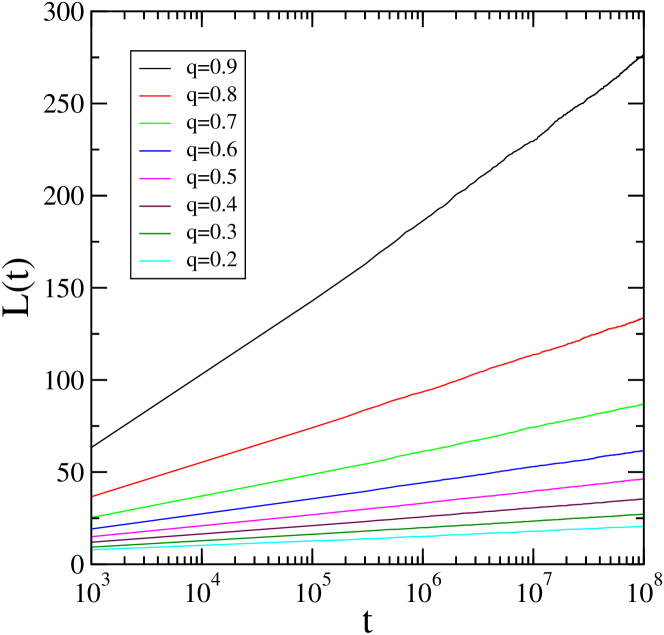
Figure 3: (Color online) Time-dependent average domain size for the domain model for various values of the rate $q$. Logarithmic growth is observed where the slopes in the log-linear plot increase with $q$. The data result from averaging over at least 100 independent runs. For a fixed time $t$ the domain size is larger the larger the value of the rate $q$ is.

IV.2 Autocorrelation

For the autocorrelation we proceed as for the original $ABC$ model. Using Eq. (5) we compute $C(t,s)$ for various waiting times $s$ and plot the data as a function of $L(t)/L(s)$. The result is shown in Fig. 4 for two values of $q$. In all cases we achieve perfect data collapse when plotting the data in this way, see Fig. 4b and 4d. This vindicates the simple aging scaling form (3) also for systems with anomalous slow dynamics. As for the autocorrelation only configurations at different stages of the time evolution are compared, we expect to encounter for that quantity the same scaling in other systems characterized by a single length scale that grows logarithmically with time, including disordered ferromagnets and spin glasses in their asymptotic regime.

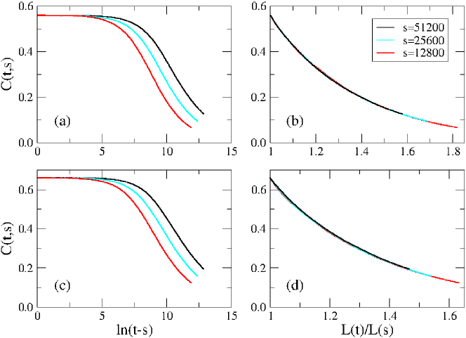
Figure 4: (Color online) Autocorrelation function for the $ABC$ model with (a,b) $q=0.9$ and (c,d) $q=0.7$. Plotting the autocorrelation against the scaling variable $L(t)/L(s)$, see (b) and (d), yields a perfect data collapse. The data result from averaging over 50000 independent runs.

IV.3 Different responses

Changes in the relaxation process due to external perturbations are best captured through the study of two-times response functions. For spin systems, as for example ferromagnets or spin glasses, one of the often used protocols, both in theoretical book10 and experimental Vin06 ; Muk10 studies, consists of applying a (random) magnetic field at the moment of a temperature quench. This field is then removed after the waiting time and the relaxation of the system is monitored.

For the domain model we employ a similar scheme for the computation of the response. Preparing the system in the same way as for the calculation of the autocorrelation, we let the system initially evolve with a given exchange rate $q=q_{i}$. At time $t=s$ we change the exchange rate to its final value $q=q_{f}$ that is kept constant until the end of the run. Due to the initial value of $q$, the average domain size at the waiting time $s$ differs from the typical domain size encountered in a system that evolves at the fixed value $q=q_{f}$. Consequently we choose as our observable the difference in system sizes between the perturbed system, where we switch from $q_{i}$ to $q_{f}$, and the unperturbed system, where $q=q_{f}$ for the whole run:

$$M(t,s)=\left|L_{p}(t,s)-L(t)\right|~{}.$$ (8)

Here $L_{p}(t,s)$ is the actual domain size of the perturbed system, whereas $L(t)$ is the average domain size without a perturbation. As in the long time limit $L_{p}(t,s)\longrightarrow L(t)$, this quantity vanishes for long observation times. The absolute values are used in Eq. (8) as we can have either that $L_{p}(s,s)>L(s)$ or that $L_{p}(s,s)<L(s)$, depending on whether $q_{i}>q_{f}$ or $q_{i}<q_{f}$. In our study we considered multiple cases with various combinations of $q_{i}$ and $q_{f}$. In doing so, we restricted ourselves to values of $q_{i}\geq 0.7$ as well as to not too large changes in $q$, such that $\left|q_{i}-q_{f}\right|\leq 0.1$.

Let us mention that the response $M(t,s)$ is a time integrated global response as (a) it sums up all the changes that accumulate over the time during which the perturbation is switched on and (b) it gives the global response of the system to a perturbation that affects all parts of the system in the same way. As such it is related in a rather complicated way to the response $R(t,s)$ discussed previously, which is the local response to an instantaneous perturbation. It is not clear a priori whether a scaling form like that given in (4) remains valid for the more complicated response studied here.

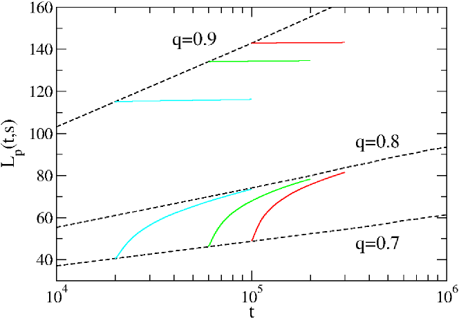
Figure 5: (Color online) Time evolution of the average growth length when changing after the waiting time $s$ the value of the rate $q$ from 0.9 to 0.8 (upper full colored lines) or from 0.7 to 0.8 (lower full colored lines). The different waiting times are s=20000 (cyan lines), s=60000 (green lines), and $s=100000$ (red lines).

Let us start with a discussion of the time evolution of the domain length $L_{p}(t,s)$ after changing the value of the rate $q$. As we see in Fig. 5 for two cases with $q_{f}=0.8$, the behavior of $L_{p}(t,s)$ is remarkably different depending on whether $q$ is decreased or increased. When decreasing $q$ after the waiting time, see the upper colored curves in Fig. 5, the domain size is at the moment of the change much larger than the average domain size in the unperturbed system that evolves at the constant value $q=q_{f}$. As a result domains grow extremely slowly after the change and it takes a very long time for $L_{p}(t,s)$ to approach the unperturbed curve $L(t)$. A closer inspection reveals that the difference $L_{p}(t,s)-L(s)$ varies logarithmically with time, $L_{p}(t,s)-L(s)=\mu\ln t+\nu$, where $\mu$ is found to be independent of the waiting time $s$. The situation is very different for cases where $q$ is increased, see the lower colored curves in Fig. 5. In these cases accelerated growth sets in and the perturbed curve approaches the unperturbed curve very rapidly. Indeed, after an initial short time regime, the difference between the two lengths $L_{p}(t,s)$ and $L(t)$ vanishes in an approximately algebraic way, with an effective exponent whose value is between 1.7 and 1.9, depending on the waiting time $s$.

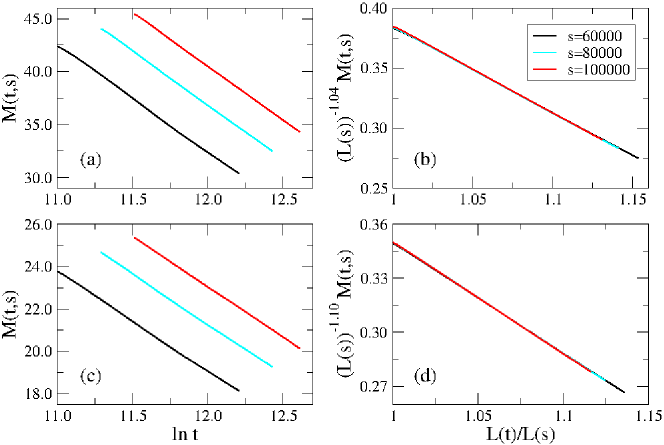
Figure 6: (Color online) Response function for the $ABC$ model where at the waiting time $s$ the exchange rates are decreased from some initial value $q_{i}$ to the final value $q_{f}$: (a,b) $q_{i}=0.9$ and $q_{f}=0.85$, (c,d) $q_{i}=0.8$ and $q_{f}=0.7$. Plotting the response function against the scaling variable $L(t)/L(s)$, see (b) and (d), yields a perfect data collapse. The data result from averaging over 10000 independent runs.

We investigate the possible scaling behavior of the response $M(t,s)$, see Eq. (8), in Figures 6 and 7. The case $q_{i}>q_{f}$ is illustrated in Fig. 6 by two examples: a change from $q_{i}=0.9$ to $q_{f}=0.85$ as well as a change from $q_{i}=0.8$ to $q_{f}=0.7$. We first remark, see Fig. 6a and 6c, that $M(t,s)$ indeed varies linearly with $\ln t$, independent of the waiting time $s$. This observation already suggests that the time integrated response also exhibits a scaling behavior where the time dependence is completely captured through the dynamic correlation length $L(t)$:

$$M(t,s)=\left(L(s)\right)^{-\alpha}f_{M}\left(\frac{L(t)}{L(s)}\right)$$ (9)

with the scaling variable $\frac{L(t)}{L(s)}$. As shown in Fig. 6b and 6d this indeed yields a data collapse of the time integrated response, with an exponent $\alpha$ that depends on the rates $q_{i}$ and $q_{f}$: $\alpha=1.04(2)$ when changing the rate from 0.9 to 0.85 and $\alpha=1.10(2)$ when changing the rate from 0.8 to 0.7. It therefore follows that for the case $q_{i}>q_{f}$ the response shows a standard aging scaling, similar to the autocorrelation, provided that the time-dependent length $L(t)$ is used.

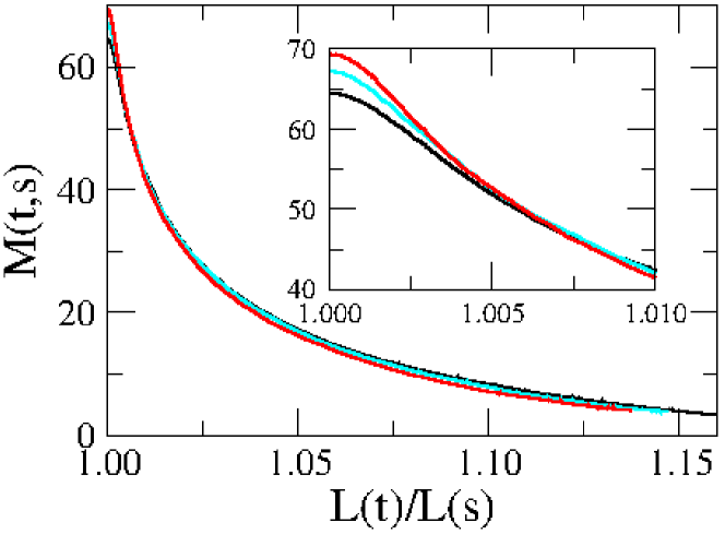
Figure 7: (Color online) Response function for the $ABC$ model where at the waiting time $s$ the exchange rate is increased from the initial value $q_{i}=0.8$ to the final value $q_{f}=0.9$. The waiting times are the same as in Fig. 5. As the different curves intersect, see inset, no data collapse can be achieved by simply multiplying $M(t,s)$ with a waiting time dependent constant. The data result from averaging over 10000 independent runs.

This is completely different for the case $q_{i}<q_{f}$, see Fig. 7. As already discussed, the domains at the moment of the change of the rate are smaller than those encountered in the unperturbed system with the same number of time steps, and the larger rate $q_{f}$ yields a much higher probability for a particle to jump from one domain to another. Consequently, the domain growth proceeds very fast. As shown in Fig. 7 for the case with $q_{i}=0.8$ and $q_{f}=0.9$, no good data collapse is observed when using as scaling variable $L(t)/L(s)$. In fact, see the inset, the curves for different waiting times always cross, which of course renders a data collapse impossible. Clearly, when the approach of $L_{p}(t,s)$ to $L(t)$ is faster than logarithmic, then a scaling behavior like that observed for $q_{i}>q_{f}$ can not be expected. As mentioned before, $L(t)-L_{p}(t,s)$ displays in a certain regime an effective algebraic dependence on $t$. This might suggest that we could choose as scaling variable $t/s$. However, as this effective exponent displays a dependence on the waiting time, this also does not yield a data collapse.

Let us close this Section by mentioning a possible alternative way to probe the response of our system. Adapting a protocol discussed in Hen12 , one can consider a space dependent rate where $q_{x}=q_{0}\pm a_{x}\,\varepsilon$ is the rate at position $x$. Here, $a_{x}=\pm 1$, whereas $\varepsilon$ is a small parameter. One would then consider two different realizations with the same noise (i.e. sequence of random numbers), one where the rate is kept fixed at $q=q_{0}$ and one where the space dependent rate $q_{x}$ is used up to the waiting time, after which the constant rate $q_{0}$ is used. Comparison of the resulting configurations should then allow to monitor how the perturbed system relaxes toward the unperturbed system. This alternative protocol is very close to the standard protocol used to calculate the autoresponse in magnetic systems where a space dependent random magnetic field is applied Bar98 . It remains to be seen, however, whether this approach allows one to sample the local response with good enough statistics. We leave it to a future study to clarify this point.

V Discussion and conclusion

In recent years numerous studies have yielded a rather good understanding of aging processes governed by an algebraic growth of the unique relevant length scale. This is especially true for systems with competing ground states where phase coarsening dominates the out of equilibrium behavior in the ordered phase, thereby yielding a typical domain size that increases as a power-law of time. Perfect magnets, as embodied by the Ising or Potts models, are well studied examples. However, as soon as one adds disorder and/or frustration effects, the dynamics slows down. A series of recent numerical studies Par10 ; Cor11 ; Cor12 ; Par12 have confirmed the existence of a crossover from an initial power-law like regime to an asymptotic regime where the relevant length scale increases much slower with time. Even though it is expected that this long time regime is characterized by logarithmic growth, none of the studies in which the time evolution of the system was followed were able to fully enter this asymptotic regime. Consequently, most of the non-equilibrium relaxation properties in such a regime have not yet been explored.

Motivated by the absence of systematic studies of aging in system with logarithmic growth, we propose to follow a different route and to focus on model systems for which it is possible to access the logarithmic regime. Even though these models are not related to disordered magnetic systems, their study should allow us to gain a better understanding of the more universal properties encountered in this regime.

In this paper we have studied the $ABC$ model and a related domain model with a simplified dynamics. The $ABC$ model allows us to study the crossover from an early time regime to the logarithmic regime. The domain model, on the other hand, very rapidly displays a logarithmic growth of the domains. Therefore, using this model we can test the scaling behavior of two-times quantities like correlation and response functions.

Our study shows that in the crossover regime the correlation function can be rather complicated. Once the domains are formed and coarsening proceeds, one enters the logarithmic regime where for waiting times large enough the two-time autocorrelation starts to exhibit a scaling behavior. This scaling behavior is fully elucidated when studying the domain model. In that case we find for the autocorrelation function a standard aging scaling, provided that the time dependence is expressed through the length scale $L(t)$ that increases logarithmically with time.

In order to study the response of the system to a perturbation, we keep the swapping rate $q$, the only parameter in the model, at some initial value $q_{i}$ up to the waiting time $s$, where we then change this rate and set it equal to the final value $q_{f}$. We then compare the time evolution of the domains formed using this protocol with that of the domains that are formed when from the start the rate is set equal to $q_{f}$. The response function is then a time integrated global response to a global change in the system. Interestingly, we find different types of behavior, depending on whether the rate is decreased or increased at the waiting time. If the rate is decreased, then the difference between the domain sizes of the perturbed and unperturbed systems decreases logarithmically with time. This then yields again a simple aging scaling with the typical length $L(t)$ as scaling variable, in complete analogy to the behavior of the autocorrelation function. This is completely different when considering the case where $q$ is increased. In that case the domains of the perturbed system grow very fast and rapidly approach the size of the unperturbed system, yielding a regime where the approach to the unperturbed regime displays an effective power-law behavior, with effective exponents that depend on the waiting time. Consequently, no dynamical scaling is observed in that case.

We view the present study as a first step in the systematic study of aging properties of systems undergoing logarithmic growth. We expect additional important insights through the study of space-time quantities, like the two-times space-time correlation function. Also, up to now we restricted ourselves to the global response to a global change. In future, this should be extended to the investigation of the local response to a local perturbation.

The two models studied here have of course no direct relation with the magnetic systems that motivated our study. Still, we expect that some of the results obtained in our study should also remain valid for magnetic systems with logarithmic growth. This is especially true for the simple aging scaling with the scaling variable $L(t)/L(s)$ that is found for the autocorrelation. We expect that this is a general feature of systems undergoing anomalous slow dynamics that is characterized by a logarithmic growth of the typical domain size, including the disordered ferromagnets. Future studies of other systems displaying this type of growth should be able to substantiate this statement. Less obvious for us is whether the intriguing behavior encountered for the global response function is also a generic property. For the disordered ferromagnet the corresponding protocol would consist in letting the system relax in the presence of a magnetic field $H$, whose value is then changed after the waiting time (this final value could of course be $H=0$). We then should again have that the domains at the waiting time have a different typical length when compared with the domain size at constant magnetic field. The situation therefore seems rather similar to what is discussed in this paper. Still, the domains in two- and three-dimensional ferromagnets are very different to the pure domains encountered in the domain model. It therefore remains an intriguing question for the future whether responses in other systems with anomalous slow dynamics behave in a similar way to what has been found in our study.

- (1) M. Henkel and M. Pleimling, Non-Equilibrium Phase Transitions, Volume 2: Ageing and Dynamical Scaling Far From Equilibrium (Springer, Heidelberg, 2010).
- (2) A. J. Bray, Adv. Phys. 43, 357 (1994).
- (3) M. Henkel, J. Phys.: Condens. Matter 19, 065101 (2007).
- (4) L. F. Cugliandolo, in Slow Relaxation and Non-equilibrium Dynamics in Condensed Matter, editors J.-L. Barrat, J. Dalibard, J. Kurchan, and M. V. Feigel’man (Springer, 2003).
- (5) A. Kolton, A. Rosso, and T. Giamarchi, Phys. Rev. Lett. 95, 180604 (2005).
- (6) J. D. Noh and H. Park, Phys. Rev. E 80, 040102(R) (2009).
- (7) J. L. Iguain, S. Bustingorry, A. B. Kolton, and L. F. Cugliandolo, Phys. Rev. B 80, 094201 (2009).
- (8) C. Monthus and T. Garel, J. Stat. Mech. (2009) P12017.
- (9) M. Rao and A. Chakrabarti, Phys. Rev. Lett. 71, 3501 (1993).
- (10) C. Aron, C. Chamon, L. F. Cugliandolo, and M. Picco, J. Stat. Mech. (2008) P05016.
- (11) H. Park and M. Pleimling, Phys. Rev. B 82, 144406 (2010).
- (12) F. Corberi, L. F. Cugliandolo, and H. Yoshino, in Dynamical Heterogeneities in Glasses, Colloids, and Granular Media, edited by L. Berthier, G. Biroli, J.-P. Bouchaud, L. Cipelleti, and W. Van Saarloos (Oxford University Press, Oxford, 2011).
- (13) F. Corberi, E. Lippiello, A. Mukherjee, S. Puri, and M. Zannetti, J. Stat. Mech. (2011) P03016.
- (14) F. Corberi, E. Lippielli, A. Mukherjee, S. Puri, and M. Zannetti, Phys. Rev. E 85, 021141 (2012).
- (15) H. Park and M. Pleimling, Eur. Phys. J. B 85, 300 (2012).
- (16) D. A. Huse and C. L. Henley, Phys. Rev. Lett. 54, 2708 (1985).
- (17) M. R. Evans, J. Phys.: Condens. Matter 14, 1397 (2002).
- (18) M. R. Evans, Y. Kafri, H. M. Koduvely, and D. Mukamel, Phys. Rev. Lett. 80, 425 (1998).
- (19) M. R. Evans, Y. Kafri, H. M. Koduvely, and D. Mukamel, Phys. Rev. E 58, 2764 (1998).
- (20) M. Clincy, B. Derrida, and M. R. Evans, Phys. Rev. E 67, 066115 (2003).
- (21) T. Bodineau, B. Derrida, V. Lecomte, and F. van Wijland, J. Stat. Phys. 133, 1013 (2008).
- (22) A. Ayyer, E. A. Carlen, J. L. Lebowitz, P. K. Mohanty, D. Mukamel, and E. Speer, J. Stat. Phys. 137, 1166 (2009).
- (23) A. Lederhendler and D. Mukamel, Phys. Rev. Lett. 105, 150602 (2010).
- (24) A. Lederhendler, O. Cohen, and D. Mukamel, J. Stat. Mech. (2010) P11016.
- (25) J. Barton, J. L. Lebowitz, and E. R. Speer, J. Phys. A: Math. Theor. 44, 065005 (2011).
- (26) L. Bertini, N. Cancrini, and G. Posta, J. Stat. Phys. 144, 1284 (2011).
- (27) J. Barton, J. L. Lebowitz, and E. R. Speer, J. Stat. Phys. 145, 763 (2011).
- (28) A. Gerschenfeld and B. Derrida, EPL 96, 20001 (2011).
- (29) O. Cohen and D. Mukamel, J. Phys. A: Math. Theor. 44, 415004 (2011).
- (30) T. Bodineau and B. Derrida, J. Stat. Phys. 145, 745 (2011).
- (31) A. Gerschenfeld and B. Derrida, J. Phys. A: Math. Theor. 45, 055002 (2012).
- (32) O. Cohen and D. Mukamel, Phys. Rev. Lett. 108, 060602 (2012).
- (33) O. Cohen and D. Mukamel, arXiv:1210.3788.
- (34) R. Lahiri and S. Ramaswamy, Phys. Rev. Lett. 79, 1150 (1997).
- (35) P. F. Arndt, T. Heinzel, and V. Rittenberg, J. Phys. A: Math. Gen. 31, L45 (1998).
- (36) R. Lahiri, M. Barma, and S. Ramaswamy, Phys. Rev. E 61, 1648 (2000).
- (37) Y. Kafri, D. Biron, M. R. Evans, and D. Mukamel, Eur. Phys. J. B 16, 669 (2000).
- (38) A. Lipowski and D. Lipowska, Phys. Rev. E 79, 060102(R) (2009).
- (39) P. Calabrese and A. Gambassi, J. Phys. A: Math. Gen. 38, R133 (2005).
- (40) N. Afzal, J. Waugh, and M. Pleimling, J. Stat. Mech. (2011) P06006.
- (41) A. Ahmed, D. Konrad, and M. Pleimling, J. Stat. Mech. (2012) P07014.
- (42) E. Vincent, in Ageing and the Glass Transition, Lecture Notes in Physics 716, edited by M. Henkel, M. Pleimling, and R. Sanctuary (Springer, Berlin, Heidelberg, 2007).
- (43) T. Mukherjee, M. Pleimling, and Ch. Binek, Phys. Rev. B 82, 134425 (2010).
- (44) M. Henkel, J. D. Noh, and M. Pleimling, Phys. Rev. E 85, 030102(R) (2012).
- (45) A. Barrat, Phys. Rev. E 57, 3629 (1998).