Department of Applied Quantum Physics, Graduate School of Engineering,
Kyushu University, Fukuoka 812-8581, Japan
Abstract. We use Monte Carlo simulations to study multicritical properties of an Ising metamagnet in an external field. According to the mean field theory predictions, a three-dimensional layered metamagnet is expected to display a tricritical point decomposition to a critical endpoint and a bicritical endpoint, when a ratio between intralayer ferromagnetic and interlayer antiferromagnetic couplings becomes sufficiently small. Our simulations show no evidence of such a decomposition and produce a tricritical behaviour even for a coupling ratio as small as $R=0.01$.
$PACS\ codes$: 75.10.Hk; 75.30.Kz; 75.40.Cx; 75.40.Mg; 75.50.Ee.
$Keywords$: Ising metamagnet; Monte Carlo simulation; Multicritical behaviour; Tricritical point decomposition.

$*$Corresponding author.
Permanent address: Department of Applied Quantum Physics, Graduate School of Engineering, Kyushu University, Fukuoka 812-8581, Japan
Tel.: +81-92-642-3811; Fax: +81-92-633-6958

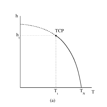
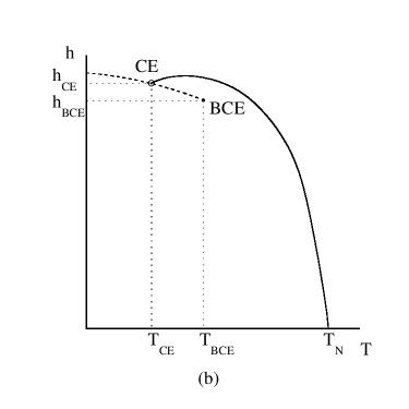
Figure 1: Schematic phase diagrams of a metamagnet displaying two different kinds of behaviour: the second-order and first-order transition lines (solid and dashed, respectively) either (a) meet at the tricritical point (TCP) or, (b) as predicted by the MFT, can end up by a critical endpoint (CE) and a bicritical endpoint (BCE).

1.Introduction
Ising metamagnets, systems with ferromagnetic and antiferromagnetic couplings simultaneously present, have attracted much interest because it is possible to induce novel kinds of critical behaviour by forcing competition between these couplings, in particular by applying a magnetic field. They are generally believed to exhibit a tricritical point (TCP) which separates a second-order phase transition at high temperatures and low fields from a first-order phase transition at low temperatures and high fields (Fig.1a). Although this picture has in principle been confirmed experimentally stryjewski , some ambiguities concerning the tricritical behaviour still remain. In particular, the mean-field theory motizuki (MFT) predicts splitting of the TCP into a critical endpoint (CE) and a bicritical endpoint (BCE) (as shown in Fig.1b), if the ratio between total intrasublattice ferromagnetic and total intersublattice antiferromagnetic couplings is sufficiently small. Such a way, for example, if we increased the field at any temperature between $T_{\mathrm{CE}}$ and $T_{\mathrm{BCE}}$, the system would first undergo a first-order transition from an antiferromagnetic phase to a generally different antiferromagnetic phase, and then a second-order transition to a paramagnetic phase. Since, as we know, the MFT neglects fluctuations, which could destroy this “middle” phase, some more sophisticated methods have been employed to give an answer to the question of whether the kind of phase diagram shown in Fig.1b can really exist or not. However, no definite conclusions have been drawn yet. So far, a two-dimensional next-nearest neighbor model ($nnn-model$) for Ising antiferromagnet has been studied by a Monte Carlo renormalization group landau-swendsen (MCRG) with no indications of the TCP splitting, however, transfer matrix techniques herrmann did not reproduce (possibly because of the limited strip widths which could be studied) tricritical behaviour at very small ratios R. The same model has been also studied in three dimensions, which is more interesting case from the experimental point of view as well as from such a respect that fluctuations are smaller than in two dimensions and hence, the MFT predictions are more likely to be correct. Monte Carlo (MC) and MCRG methods applied to a variety of Hamiltonians for both $meta-model$ and $nnn-model$ of an Ising antiferromagnet showed that the exponent behaviour was consistent with the MFT, however, could not detect any change in the phase diagram itself her-ras-lan . However, more recent MC simulations on $nnn-model$ produced only tricritical behaviour for $R\geq 0.05$ herrmann-landau , i.e. the result contradicting to the MFT predictions.
Clear distinction in critical behaviour between two- and three-dimensional models was observed in the antiferromagnetic Blume-Capel model, which, according to the MFT, should also show decomposition of the TCP. While MC simulations produced only tricritical behaviour in two dimensions kim-bla-car-wan , they provided clear evidence of the decomposition into a CE and a BCE in a three-dimensional model wang-kimel . In light of the previous studies on Ising metamagnets, which seemed to favor a non-decomposition of the TCP, quite perplexing results have been recently obtained by both experimental kleemann1 -kleemann3 and Monte Carlo selke-dasgupta -pleimling-selke studies on one of the typical Ising metamagnets - $\mathrm{FeBr_{2}}$. Although they failed to confirm the decomposition of the TCP, they quite convincingly showed the existence of anomalies of the magnetization and the specific heat, which could be associated with the decomposition. These anomalies were attributed to the effectively weak ferromagnetic intralayer interaction and the high interlayer coordination - features present in the real compound.
In this paper, we perform high precision MC simulations and provide convincing evidence of the stability of the tricritical point in the three-dimensional $meta-model$ of an Ising metamagnet for $R\geq 0.01$. Such a way, we show that merely weak, or even extremely weak, ferromagnetic intralayer interaction should not cause decomposition of the TCP, as predicted by the MFT. Hence, in light of the previous results obtained for $\mathrm{FeBr_{2}}$, the high interlayer coordination, which is present in the real compound but absent in our model, seems to be of crucial importance in producing of such a decomposition, if it really takes place.
2.Model and simulation technique
The considered system is the spin-$\frac{1}{2}$ Ising metamagnet described by the Hamiltonian

$$H=-J_{1}\sum_{<i,j>}s_{i}s_{j}-J_{2}\sum_{<i,k>}s_{i}s_{k}-h\sum_{i}s_{i}\ ,$$ (1)

where $s_{i}=\pm 1$ is an Ising spin, $<i,j>$ and $<i,k>$ denote the sum over nearest neighbors in the plane and in adjacent planes, respectively, and $h$ is an external magnetic field. We choose $J_{1}>0$ and $J_{2}<0$ so that each of the planes is ferromagnetic, but antiferromagnetically coupled to adjacent planes.
According to the MFT scenario, it is only the ratio $R=z_{1}J_{1}/z_{2}|J_{2}|$, where $z_{1}$ and $z_{2}$ are numbers of nearest neighbors of the site $i$ in the plane and adjacent planes, respectively, which determines the phase diagram. While for $R>\frac{3}{5}$ it should look like the one in Fig.1a, i.e. it should display a TCP with tricritical exponents $\alpha_{t}=\frac{1}{2},\beta_{t}=\frac{1}{4},\gamma_{t}=1,\lambda_{t}=\frac{1}{2}$, for $0<R<\frac{3}{5}$ the TCP is expected to split up into a CE and a BCE, as shown in Fig.1b. Then, in the latter case, both the CE and the BCE should probably keep usual three-dimensional critical exponents: $\alpha\approx 0.11,\beta\approx 0.32,\gamma\approx 1.24$. At $R=\frac{3}{5}$ the MFT predicts a four-order critical point with yet different set of exponents.
We have performed MC simulations on simple cubic lattice samples of linear sizes ranging from $L$ = 16 to $L$= 40, assuming the periodic boundary condition throughout. We used an antiferromagnetic initial spin configuration at low temperatures and the field not exceeding the critical value $h_{c}(p)=pz_{2}|J_{2}|$, and a ferromagnetic one at high temperatures. As we moved in the temperature-field $(T,h)$ space, we used the last spin configuration as an input for calculation at the next point. Spin updating followed a Metropolis dynamics. Averages were calculated using at most 25,000 Monte Carlo steps per spin (MCS/s) after equilibrating over another 5,000 to 10,000 MCS/s. Since we focused on the tricritical region, which for very small ratios $R$ lies at very low temperatures, in order to prevent huge fluctuations at field-heating and field-cooling processes (the path of measurement would be virtually parallel to the phase boundary), we only performed $(h\uparrow)$+$(h\downarrow)$ loops, i.e. raised and lowered the field at fixed temperature and measured :
the direct and staggered magnetizations $m$ and $m_{s}$, respectively

$$m=\langle M\rangle/N,\ {\mathrm{where}}\ M=|\sum_{i\in{\mathrm{A}}}s_{i}+\sum_{j\in{\mathrm{B}}}s_{j}|\ ,$$ (2)

$$m_{s}=\langle M_{s}\rangle/N,\ {\mathrm{where}}\ M_{s}=|\sum_{i\in{\mathrm{A}}}s_{i}-\sum_{j\in{\mathrm{B}}}s_{j}|\ ,$$ (3)

where $N$ is a total number of sites, and A, B denote sublattices made up of ”spin-up” and ”spin-down” planes, respectively,
and the corresponding direct and staggered susceptibilities per site $\chi$ and $\chi_{s}$, respectively

$$\chi=\frac{(\langle M^{2}\rangle-\langle M\rangle^{2})}{Nk_{B}T}\ ,$$ (4)

$$\chi_{s}=\frac{(\langle M_{s}^{2}\rangle-\langle M_{s}\rangle^{2})}{Nk_{B}T}\ .$$ (5)

These quantities were used to determine the nature as well as a location of the transition. The simulations were performed on the vector supercomputer FUJITSU VPP700/56.
3.Results and discussion
We studied phase transitions of the system for four different values of $R$: 0.5, 0.2, 0.05 and 0.01, with particular attention paid to the region of the expected TCP. Fig.2 depicts phase boundaries in the vicinity of the TCPs for the respective values of $R$. At sufficiently low temperatures, both the direct and staggered magnetizations displayed besides jumps also pronounced hysteresis formed by the $(h\uparrow)$+$(h\downarrow)$ cycles - features which are characteristic for a first-order transition. In Fig.2 the upper and lower branches in the low temperature region (blank circles) are determined by the jumps of the $m_{s}$ curve in the $(h\uparrow)$ and $(h\downarrow)$ processes, respectively, and outline the region of the coexistence of the antiferromagnetic and ferromagnetic phases. Increasing temperature makes the hysteresis shrink, and eventually disappear at a point which gave us a first guess for the location of the TCP (arrows). Note, however, that if this is not done for sufficiently large $L$, the above mentioned phenomena, accompanying first-order transitions, could be suppressed by the finite-size effects, and hence, lattices of small $L$ are not suitable for such a kind of investigation. Upon further increase in temperature, the $(h\uparrow)$ and $(h\downarrow)$ magnetization curves collapse onto a single smooth curve, signifying a second-order transition (filled circles). Its location was determined by the location of the staggered susceptibility peak, extrapolated for $L$ brought to infinity. As we can see, none of the cases shown in Fig.2 shows any indications of the TCP decomposition. On the other hand, according the MFT the splitting should take place in each of the cases and in very noticeable scale (e.g., for $R=0.05$ the separation between the CE and BCE temperatures is estimated to $50\%$). Note that, in contrast to the results obtained for the three-dimensional $nnn-model$ herrmann-landau , the varying value of $R$ has virtually no influence on the slope of the transition in the tricritical region (however, it is not possible to see it right away from Fig.2 because of different scales).
At this stage, judging by the obtained results, we could draw a preliminary conclusion that there is no decomposition of the TCP in this model, at least for $R\geq 0.01$. In order to confirm this claim, we picked up the case of $R=0.01$ (it is the most likely candidate for the decomposition, if there is any) and investigated it more closely. In particular, we ran additional simulations for lattices of larger $L$ and finally extrapolated to $L\rightarrow\infty$. This data presented on a fine scale allowed us to localize the TCP with fairly high accuracy to $(k_{B}T_{t}/|J_{2}|,h_{t}/|J_{2}|)=(0.0150\pm 0.0001,1.999138\pm 0.000002)$. Then we examined behaviour of some physical quantities as they approach the TCP. Fig.3 depicts a log-log plot of the direct and staggered susceptibilities vs field near the TCP. While a good fit to a power-low behaviour can be observed in a fairly narrow region quite near the TCP, a more distant region shows a deviation from such a behaviour, probably as a consequence of logarithmic corrections predicted for tricritical point in three dimensions wegner-riedel . Nevertheless, slopes of the both lines seem to asymptotically approach the magnitude close to 1 and $\frac{1}{2}$ for $\chi_{st}$ and $\chi$, respectively. This means, however, that both the staggered and direct susceptibilities take on exponents which are very close to the tricritical ones $\gamma_{t}=1$ and $\lambda_{t}=\frac{1}{2}$ rather than those which characterize an usual critical behaviour. These results just confirm the previous conclusion about non-decomposition of the TCP and put it on firmer ground.
In Fig.4 we depict both the tricritical temperature and the tricritical field vs $R$. While the tricritical temperature shows a linear dependence over whole range of $R$, which for a certain smaller range of $R$ was also observed in a diluted $nnn-model$ galam , the tricritical field displays a slight curvature. As expected, for $R\rightarrow 0$, the tricritical temperature moves to zero, while the tricritical field approaches the exact value for the zero-temperature critical field $h_{c}(0)/|J_{2}|=z_{2}(=2)$.
4.Conclusions
We have investigated the possibility of the decomposition of the tricritical point in a three-dimensional layered Ising metamagnet. Since the mean-field theory predicts such a decomposition for small values of the ratio $R$, we mainly focused on that region. However, we observed only tricritical behaviour with no signs of the decomposition for $R\geq 0.01$. In the case of the smallest value of $R=0.01$, where, according to the MFT, the TCP is most likely to decompose, we managed to locate the TCP with a precision of approximately $1\%$ in temperature and $0.0001\%$ in the field. Even for such a small $R$ the analysis of the critical exponents clearly showed tricritical behaviour. Therefore, we conclude that it is very unlikely that the TCP decomposes for any value of $R$, although some very small possibility of the decomposition for $R<0.01$ still remains. Hence, recently found anomalies in $\mathrm{FeBr_{2}}$ (note that it has relatively high value of $R$ aru-kats-kat ; selke-dasgupta ) make us believe that the high interlayer coordination (interlayer superexchange paths present in the real material), supposedly causing the anomalies by inducing local thermal excitations of the second antiferromagnetic phase for weak intralayer couplings $J_{1}$, could play a key role in the possible TCP decomposition.

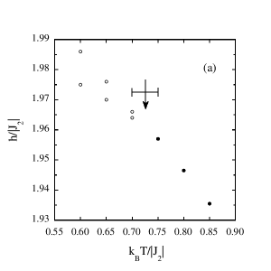
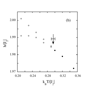
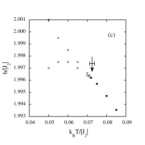
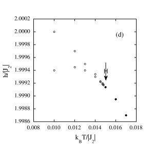
Figure 2: Phase diagrams near the TCP in the $T-h$ plane for four different values of $R$: (a) 0.5, (b) 0.2, (c) 0.05 and (d) 0.01. The TCP (arrow) separates second-order transitions (filled circles) from first-order transitions (blank circles).

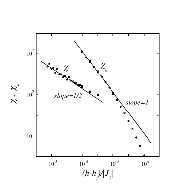
Figure 3: Log-log plot of the direct and staggered susceptibilities $\chi$ and $\chi_{st}$, respectively, as a function of $(h-h_{t})/|J_{2}|$ for $k_{B}T/|J_{2}|=0.0150$, $h_{t}/|J_{2}|=1.999138$ and $R=0.01$. The crosses and the diamonds represent data for two different lattice sizes $L=30$ and $L=40$, respectively, and the solid lines of slopes 1/2 and 1 (expected tricritical exponents for $\chi$ and $\chi_{st}$, respectively) serve as guides to the eye.

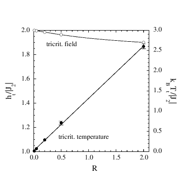
Figure 4: Tricritical temperature $k_{B}T_{t}/|J_{2}|$ and tricritical field $h_{t}/|J_{2}|$ as functions of the ratio $R$. Vertical bars indicate errors and are only shown when they exceed the sizes of the symbols.

References

- (1) E. Stryjewski and N. Giordano, Adv. Phys. 26, 487, (1977).
- (2) K. Motizuki, J. Phys. Soc. Japan 14, 759, (1959).
- (3) D. P. Landau and R. H. Swendsen, Phys. Rev. B 33, 7700, (1986).
- (4) H. J. Herrmann, Phys. Lett. 100A, 256, (1984).
- (5) H. J. Herrmann, E. B. Rasmussen and D. P. Landau, J. Appl. Phys. 53, 7994, (1982).
- (6) H. J. Herrmann and D. P. Landau, Phys. Rev. B 48, 239, (1993).
- (7) J. D. Kimel, S. Black, P. Carter and Y.-L. Wang, Phys. Rev. B 35, 3347, (1987).
- (8) Y.-L. Wang and J. D. Kimel, J. Appl. Phys. 69, 6176, (1991).
- (9) M. M. P. de Azevedo, Ch. Binek, J. Kushauer, W. Kleemann and D. Bertrand, J. Magn. Magn. Mater. 140-144, 1557, (1995).
- (10) J. Pelloth, R. A. Brand, S. Takele, M. M. P. de Azevedo, W. Kleemann, Ch. Binek, J. Kushauer and D. Bertrand, Phys. Rev. B 52, 15372, (1995).
- (11) H. Aruga Katori, K. Katsumata and M. Katori, Phys. Rev. B 54, R9620, (1996).
- (12) K. Katsumata, H. Aruga Katori, S. M. Shapiro and G. Shirane, Phys. Rev. B 55, 11466, (1997).
- (13) O. Petracic, Ch. Binek and W. Kleemann, J. Appl. Phys. 81, 4145, (1997).
- (14) W. Selke and S. Dasgupta, J. Magn. Magn. Mater. 147, L245, (1995).
- (15) W. Selke, Z. Phys. B 101, 145, (1996).
- (16) M. Pleimling and W. Selke, Phys. Rev. B 56, 8855, (1997).
- (17) F. J. Wegner and E. K. Riedel, Phys. Rev. B 7, 248, (1973).
- (18) S.Galam, P.Azaria and H.T.Diep, J. Phys.: Condens. Matter 1, 5473, (1989).