Spectral and transport properties of the
two-dimensional Lieb lattice

Abstract

The specific topology of the line centered square lattice (known also as the Lieb lattice) induces remarkable spectral properties as the macroscopically degenerated zero energy flat band, the Dirac cone in the low energy spectrum, and the peculiar Hofstadter-type spectrum in magnetic field. We study here the properties of the finite Lieb lattice with periodic and vanishing boundary conditions. We find out the behavior of the flat band induced by disorder and external magnetic and electric fields. We show that in the confined Lieb plaquette threaded by a perpendicular magnetic flux there are edge states with nontrivial behavior. The specific class of twisted edge states, which have alternating chirality, are sensitive to disorder and do not support IQHE, but contribute to the longitudinal resistance. The symmetry of the transmittance matrix in the energy range where these states are located is revealed. The diamagnetic moments of the bulk and edge states in the Dirac-Landau domain, and also of the flat states in crossed magnetic and electric fields are shown.

I Introduction

The interest in the line centered square lattice, known as the 2D Lieb lattice, comes from the specific properties induced by its topology. The lattice is characterized by a unit cell containing three atoms, and a one-particle energy spectrum showing a three band structure with electron-hole symmetry, one of the branches being flat and macroscopically degenerate. For the infinite lattice, the three energy bands touch each other at the middle of the spectrum (taken as the zero energy ), and the low energy spectrum exhibits a Dirac cone located at the point $\Gamma=(\pi,\pi)$ in the Brillouin zone. Except for the presence of the flat band, the Lieb lattice shows similarities with the honeycomb lattice in what concerns both spectral and transport properties. For instance, besides the presence of the Dirac cone, the energy spectrum in the presence of the magnetic field shows also a double Hofstadter picture, with the typical $\sqrt{B}$ dependence of the relativistic bands on the magnetic field $B$ Rammal . The Hall resistance of the two systems in the quantum regime behaves alike, but the step between consecutive plateaus equals $h/e^{2}$ in the Lieb case (instead of $h/2e^{2}$ for graphene) because of the presence of a single Dirac cone per BZ. An all-angle Klein transmission is proved by the relativistic electrons in the Lieb lattice Aoki ; Goldman ; Shen .

There are more lattices that support flat bands, however it is specific to the Lieb lattice that the band is robust against the magnetic field, while other lattices develop dispersion at any $B\neq 0$. The intrinsic spin-orbit coupling does not affect the flat band either, but opens a gap at the touching point $\Gamma$, the Lieb system becoming in this way a quantum spin Hall phase Goldman ; Weeks . Topological phase transitions driven by different parameters are studied in Smith ; Tsai . The zero-energy flat bands became a topic of intense study also for other reasons: they may allow for the non-Abelian FQHE Wang ; DasSarma ; Bergholtz or for ferromagnetic order and surface superconductivity Zhang ; Zhao ; Volovik .

In this paper we address the properties of the finite (mesoscopic) Lieb lattice with emphasis on some features of the flat band and of the edge states which are specific to this lattice. We adopt the spinless tight-binding approach, and the spectral properties are examined under both periodic and vanishing boundary conditions applied to the system described in Fig.1. In section II we find that the zero energy flat band exists independently of the boundary conditions. It turns out, however, that in the periodic case the band is built up only from B- and C- orbitals, while in the other case the A-type orbitals are also involved (see Fig.1). We prove this analytically by calculating the eigenfunction in both situations. In this way we also find out that for confined systems (i.e., with vanishing boundary conditions) the degeneracy of the flat band equals $N_{cell}+1$ ($N_{cell}$ is the number of cells of the mesoscopic plaquette). We find in section IIIA that for a confined plaquette two levels separate from the bunch when a perpendicular magnetic field is applied, such that the degeneracy is reduced by 2. This is proved in a perturbative manner for the general case, however it can be observed more easily by the use of the toy model consisting of two cells only.

Next, we study how the flat band degeneracy is lifted by disorder and by an external electric field applied in-plane. An exotic result is that the extended states of the disordered flat band in the presence of a magnetic field behave according to the orthogonal Wigner-Dyson distribution although the unitary distribution is expected. When an electric field is applied, the flat band splits in a Stark-Wannier ladder whose structure is analyzed by calculating the diamagnetic moments of the states in crossed electric and magnetic fields.

In section IIIB we study the edge states which fill the gaps of the double Hofstadter butterfly when the magnetic field is applied on the confined Lieb plaquette. We identify three types of such states. The conventional edge states located between the Bloch-Landau bands and also between Dirac-Landau bands (i.e., the relativistic range of the spectrum) differ, as expected, in their chirality. Additionally, we detect twisted edge states situated in the magnetic gap which protect the zero-energy band, coming in bunches and characterized by an oscillating chirality as function of the magnetic field. The twisted edge states show remarkable properties: surprisingly, they are not robust to disorder, as the other types of edge states are, and does not carry transverse current (i.e., the QHE vanishes in the energy range covered by these states). The last property comes from a specific symmetry of the transmittance matrix which is discussed in section IV.

Finally, one has to note that the line centered square lattices are found in nature as $Cu-O_{2}$ Lieb planes in cuprate superconductors, and can be engineered as an optical lattice Goldman ; Manninen .

II The tight-binding model for the Lieb lattice : periodic versus vanishing boundary conditions

Our aim is to point out specific aspects of the confined Lieb plaquette from the point of view of spectral and transport properties. In order to allow for a comparison we shortly describe also the case of the infinite system, with and without magnetic field, although the eigenvalue problem is already known from the literature. We remind that the continuous model for the infinite Lieb system in perpendicular magnetic field Goldman , shows the $\sqrt{B}$ dependence on the magnetic field of the eigenenergies in the relativistic range. The information obtained in the long-wave approximation of the Schrödinger equation, concerning the dependence on $B$ of the Bloch-Landau or Dirac-Landau bands are recaptured in the spectrum of the discrete tight-binding model (Fig.5a) together with effects coming from the periodic lattice and finite edges.

In this section, starting from the tight-binding Hamiltonian, we built up the eigenfunction of the periodic and finite Lieb plaquette, and prove the degeneracy and structure of the zero-energy flat band. The crossover from the simple Hofstadter spectrum of the simple square lattice to the Lieb spectrum characterized by a double butterfly, magnetic gap and a flat band is shown in Fig.3.

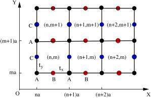
Figure 1: (Color online) The Lieb lattice: the unit cell contains three atoms $A,B$ and $C$; indices (n,m) identify the cell; $t_{x},t_{y}$ are the hopping integrals along the directions $Ox$ and $Oy$, respectively; $a$ is the lattice constant.

The Lieb lattice is a 2D square lattice with centered lines as shown in Fig.1. It is characterized by three atoms ($A,B,C$) per unit cell, the connectivity of the atom $A$ being equal to four, while the connectivity of atoms $B$ and $C$ equals two.

Introducing creation $\{a^{\dagger}_{nm},b^{\dagger}_{nm},c^{\dagger}_{nm}\}$ and annihilation $\{a_{nm},b_{nm},c_{nm}\}$ operators of the localized states $|A_{nm}>,|B_{nm}>,|C_{nm}>$  (where $(nm)$ stands for the cell index and the letters $A,B,C$ identify the type of atom),  the spinless tight-binding Hamiltonian of the Lieb lattice in perpendicular magnetic field reads:

$$H=\sum_{nm}E_{a}a^{\dagger}_{nm}a_{nm}+E_{b}b^{\dagger}_{nm}b_{nm}+E_{c}c^{\dagger}_{nm}c_{nm}$$

$$+t_{x}e^{-i\pi m\phi}a^{\dagger}_{nm}b_{nm}+t_{x}e^{i\pi m\phi}a^{\dagger}_{nm}b_{n-1,m}+t_{y}a^{\dagger}_{nm}c_{nm}+t_{y}a^{\dagger}_{nm}c_{n,m-1}$$

$$+t_{x}e^{-i\pi m\phi}b^{\dagger}_{nm}a_{n+1,m}+t_{x}e^{i\pi m\phi}b^{\dagger}_{nm}a_{nm}+t_{y}c^{\dagger}_{nm}a_{nm}+t_{y}c^{\dagger}_{nm}a_{nm+1},$$ (1)

where $\phi$ is the flux through the unit cell of the Lieb lattice measured in quantum flux units; we mention that the vector potential has been chosen as $\vec{A}=(-By,0,0)$.

The presence of a spectral flat band can be noticed already in the simplest case of the periodic boundary conditions and vanishing magnetic flux. Assuming that the lattice is composed of $N_{cell}^{x}=N$ cells along $Ox$ and $N_{cell}^{y}=M$ cells along $Oy$, the Fourier transform $c_{\vec{k}}=c_{k_{x},k_{y}}=\frac{1}{\sqrt{NM}}\sum_{n,m}c_{nm}e^{i(k_{x}n+k_{y}m)}$  (and similarly for all the other operators) yields the $k$-representation of the Hamiltonian described by a $3\times 3$ matrix:

$$H=\sum_{\vec{k}}\left(\begin{array}[]{ccc}a^{\dagger}_{\vec{k}}{}&b^{\dagger}_{\vec{k}}{}&c^{\dagger}_{\vec{k}}\end{array}\right)\left(\begin{array}[]{ccc}E_{a}&\Delta^{*}(k_{x})&\Lambda^{*}(k_{y})\\ \Delta(k_{x})&E_{b}&0\\ \Lambda(k_{y})&0&E_{c}\end{array}\right)\left(\begin{array}[]{c}a_{\vec{k}}\\ b_{\vec{k}}\\ c_{\vec{k}}\end{array}\right),$$ (2)

where $k_{x}=2\pi p/N~{}(p=1,..,N)$, $k_{y}=2\pi q/M~{}(q=1,..,M)$, and the notations $\Delta(k_{x})=t_{x}(1+e^{ik_{x}})$ , $\Lambda(k_{y})=t_{y}(1+e^{ik_{y}})$ has been used. With the choice $E_{a}=E_{b}=E_{c}=0$, one obtains the following eigenvalues:

$$\Omega_{\pm}(\vec{k})= \pm\sqrt{|\Delta|^{2}+|\Lambda|^{2}}\ =\pm 2\sqrt{t_{x}^{2}cos^{2}(k_{x}/2)+t_{y}^{2}cos^{2}(k_{y}/2)},~{}~{}$$

$$\Omega_{0}(\vec{k})= 0,$$ (3)

where $\Omega_{\pm}$ are the energies of the upper and lower band, respectively, and $\Omega_{0}$ is the nondispersive (flat) band of the Lieb lattice. The most interesting point in the BZ is the point $\Gamma=(\pi,\pi)$, where in the case of the infinite lattice the three branches are touching each other. The expansion of the functions $\Delta(k_{x})$ and $\Lambda(k_{y})$ about this point gives rise to a Dirac cone (massless) spectrum:

$$\Omega_{\pm}=\pm\sqrt{t_{x}^{2}k_{x}^{2}+t_{y}^{2}k_{y}^{2}}.$$ (4)

On the other hand, the expansion of the same functions about $R=(0,0)$ shows a parabolic dependence:

$$\Omega_{\pm}=\pm\big{(}\frac{k_{x}^{2}}{2m_{x}}+\frac{k_{y}^{2}}{2m_{y}}\big{)},$$ (5)

where $m_{x},m_{y}$ are effective masses along the two directions.

Other relevant points in the BZ are $M=(\pi,0)$ and $(0,\pi)$, which prove to be saddle points in the spectrum as it can be noticed also in Fig.2. Above and below the corresponding energy $E=\pm 2t$ (where we considered $t_{x}=t_{y}=t$) the effective mass exhibits opposite signs inducing the change of sign of the Hall effect which is visible in Fig.15.

For comparison’s sake, we remind that the energy spectrum of the honeycomb lattice contains two cones per BZ, and that the saddle point occurs at the energy $E=\pm t$. The tight-binding spectrum of the graphene extends over the interval [-3t,3t], while for the Lieb lattice the interval is [$-2\sqrt{2}t,2\sqrt{2}t$].

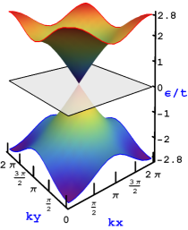
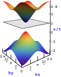
Figure 2: (Color online) The energy spectrum of the infinite Lieb lattice. (left) The case $E_{a}=E_{b}=E_{c}=0$ when the three bands (two dispersive and one flat) get in contact at $\vec{k}=(\pi,\pi)$. At low energy the dispersion is linear giving rise to Dirac cones. (right) The staggered case $E_{a}=0,E_{b}=E_{c}=1$ when the spectrum is gapped and the rounding of cones is obvious.

In order to get supplementary information about the origin of the flat band let us consider the staggered case $E_{a}=0,E_{b}=E_{c}=E_{0}$. Then, a gap is expected in the energy spectrum, and, indeed, the eigenvalues are now Shen :

$$\Omega_{\pm}(\vec{k})=\frac{1}{2}\big{[}E_{0}\pm\sqrt{E_{0}^{2}+4(|\Delta|^{2}+|\Lambda|^{2})}~{}\big{]},~{}~{}\Omega_{0}(\vec{k})=E_{0}.$$ (6)

The new spectrum is shown in Fig.2b, where one notices the persistence of the flat band, which is however shifted to $E=E_{0}$. Since the energy $E=E_{0}$ corresponds to the atomic level of the orbitals $B$ and $C$, the result argues that the flat band states are created only by this type of orbitals. The gap induced by the staggered arrangement is accompanied by the rounding of the cones, that indicates a non-zero effective mass in the low-energy range of the two spectral branches, as it can be observed in Fig.2b.

In what follows we shall calculate the eigenfunctions of the finite Lieb lattice, imposing first periodic conditions, and then the vanishing boundary conditions proper to the confined plaquette. Let $\Psi_{\vec{k}}$ be the eigenfunctions of the Lieb lattice with periodic boundary conditions built up as the linear combination:

$$\Psi_{\vec{k}}=\alpha_{\vec{k}}a^{\dagger}_{\vec{k}}|0>+\beta_{\vec{k}}b^{\dagger}_{\vec{k}}|0>+\gamma_{\vec{k}}c^{\dagger}_{\vec{k}}|0>,$$ (7)

where the coefficients $\alpha_{\vec{k}},\beta_{\vec{k}},\gamma_{\vec{k}}$ satisfy the equations:

$$E_{a}\alpha_{\vec{k}}+ \Delta^{*}(k_{x})\beta_{\vec{k}} +\Lambda^{*}(k_{y})\gamma_{\vec{k}}=E\alpha_{\vec{k}}$$ (8)

$$\Delta(k_{x})\alpha_{\vec{k}} +E_{b}\beta_{\vec{k}}=E\beta_{\vec{k}}$$

$$\Lambda(k_{x})\alpha_{\vec{k}} +E_{c}\gamma_{\vec{k}}=E\gamma_{\vec{k}}.$$

Then, the functions corresponding to the eigenvalues $\Omega_{0}$ and $\Omega_{\pm}$ in Eq.(3) read:

$$\Psi^{0}(\vec{k}) =\frac{1}{\sqrt{|\Delta|^{2}+|\Lambda|^{2}}}\big{(}\Lambda^{*}(k_{y})b^{\dagger}_{\vec{k}}-\Delta^{*}(k_{x})c^{\dagger}_{\vec{k}}\big{)}|0>$$ (9)

$$\Psi^{\pm}(\vec{k}) =\frac{1}{2}\big{(}\pm a^{\dagger}_{\vec{k}}+\frac{\Delta(k_{x})}{{\sqrt{|\Delta|^{2}|+|\Lambda|^{2}}}}~{}b^{\dagger}_{\vec{k}}+\frac{\Lambda(k_{y})}{{\sqrt{|\Delta|^{2}+|\Lambda|^{2}}}}~{}c^{\dagger}_{\vec{k}}\big{)}|0>.$$ (10)

In the case of periodic conditions applied to the finite plaquette there are some subtleties concerning the band degeneracy which become unimportant in the limit of infinite system. It is obvious from Eqs.(9-10) that the three bands come into contact at $\vec{k}=(\pi,\pi)$, however this value of $\vec{k}$ is allowed only if both $N$ and $M$ are even. In this case the flat band at $E=0$ is ($N_{cell}+2$)- fold degenerate, otherwise all the three bands are $N_{cell}$-fold degenerate (where the number of cells $N_{cell}=NM$).

The expression of $\Psi^{0}(\vec{k})$ in Eq.(9) indicates again that the flat band of the periodic lattice is composed only from orbitals of the type $B$ and $C$. On the other hand, we shall see below that in the case of vanishing boundary conditions the zero-energy eigenfunction may sit also on the $A-$type sites, and that the degeneracy of the flat band becomes $N_{cell}+1$.

The periodic boundary conditions can be used in the presence of a uniform perpendicular magnetic field for rational values of the magnetic flux $\phi=p/q$ resulting in a spectrum composed of two Hofstadter butterflies similar to the case of the honeycomb lattice. However, in contradistinction to the honeycomb lattice, one notices the presence of a dispersionless band at $E=0$, which is flat with respect to the variation of the magnetic flux, and is protected by a gap opened at $B\neq 0$ Aoki ; Goldman . The spectrum exhibits Bloch-Landau bands at the extremities and also relativistic Dirac-Landau bands towards the middle. The two types of bands are distinguished by opposite chirality $dE/d\phi$ and by different dependence on the magnetic field.

The periodic boundary conditions discussed above can be properly used for describing infinite lattices, however when interested in mesoscopic plaquettes they have to be replaced with vanishing boundary conditions. We intend to identify the differences introduced by the finite size, which will turn out to be non-trivial in the case of the Lieb lattice.

For the confined Lieb lattice, the eigenfunctions can be obtained as combinations of functions Eq.(9) or Eq.(10) with coefficients that ensure the vanishing of the eigenfunction along the edges. As a technical detail we mention that (along the Ox direction, for instance) the finite plaquette begins with the atom $A$ in the first cell, and also ends with an atom $A$ which belong to the $(N+1)$-th cell. This means that the wave function $|\Phi(\vec{k})>$ should vanish at the site $B$ in the $0$-th and $(N+1)$-th cell, i.e.: $<\Phi(\vec{k})|b^{\dagger}_{N+1,m}|0>=<\Phi(\vec{k})|b^{\dagger}_{0,m}|0>=0$. Similarly, the vanishing condition along Oy occurs at the site $C$ in the $0$-th and $(M+1)$-th cell along this direction, i.e.: $<\Phi(\vec{k})|c^{\dagger}_{n,M+1}|0>=<\Phi(\vec{k})|c^{\dagger}_{n,0}|0>=0$.

In the localized representation, which is the proper one in the case of confined systems, the eigenfunctions $|\Phi^{0}(\vec{k})>$ corresponding to $E=\Omega_{0}=0$ look as follows:

$$|\Phi^{0}(\vec{k})>=\sqrt{\frac{2}{N+1}}\sqrt{\frac{2}{M+1}}\sum_{n=1}^{N+1}\sum_{m=1}^{M+1}\big{(}\frac{2t_{y}cos\frac{k_{y}}{2}}{\sqrt{|\Delta|^{2}+|\Lambda|^{2}}}sink_{x}n~{}sink_{y}(m-\frac{1}{2})~{}b^{\dagger}_{nm}|0>$$

$$-\frac{2t_{x}cos\frac{k_{x}}{2}}{\sqrt{|\Delta|^{2}+|\Lambda|^{2}}}sink_{x}(n-\frac{1}{2})~{}sink_{y}m~{}c^{\dagger}_{nm}|0>\big{)},$$ (11)

where $k_{x},k_{y}$ are obtained from the condition that the wave function vanishes at the boundary, and equal $k_{x}=p\pi/(N+1)$  (p=1,..,N+1) and $k_{y}=\frac{q\pi}{M+1}$  (q=1,..,M+1). Since the situations $p=N+1$ (at any $q$) and $q=M+1$ (at any $p$), generate $|\Phi^{0}>=0$, we are left in Eq.(11) with only $NM$ non-vanishing degenerate orthogonal eigenfunction.

The eigenfunctions $|\Phi^{\pm}(\vec{k})>$ corresponding to the other two energy branches can be written similarly as:

$$|\Phi^{\pm}(\vec{k})>=\sqrt{\frac{2}{(N+1)(M+1)}}\sum_{n=1}^{N+1}\sum_{m=1}^{M+1}\big{(}\pm sink_{x}(n-\frac{1}{2})sink_{y}(m-\frac{1}{2})~{}a^{\dagger}_{nm}|0>$$

$$+\frac{2t_{x}cos\frac{k_{x}}{2}}{\sqrt{|\Delta|^{2}+|\Lambda|^{2}}}sink_{x}n~{}sink_{y}(m-\frac{1}{2})~{}b^{\dagger}_{nm}|0>$$

$$+\frac{2t_{y}cos\frac{k_{y}}{2}}{\sqrt{|\Delta|^{2}+|\Lambda|^{2}}}sink_{x}(n-\frac{1}{2})sink_{y}m~{}c^{\dagger}_{nm}|0>\big{)},$$ (12)

where states of the type $A$ are this time also present. One can readily see that the number of non-vanishing states in each spectral branch is $(N+1)(M+1)-1$, since the point $\Gamma=(\pi,\pi)$ has to be treated separately. This is because its corresponding energy vanishes and the state should be counted in the flat band. In this case the wave function becomes:

$$|\Phi^{0}_{a}>=:|\Phi^{\pm}(\pi,\pi)>=\sqrt{\frac{1}{N+1}}\sqrt{\frac{1}{M+1}}\sum_{n=1}^{N+1}\sum_{m=1}^{M+1}(-1)^{n+m}~{}a^{\dagger}_{nm}|0>.$$ (13)

For the finite Lieb plaquette with vanishing boundary conditions, one may conclude that the flat band degeneracy equals $NM+1$, while each other branch contains $NM+N+M$ states, so that the total number of states equals indeed the number of sites $3NM+2(N+M)+1$.

In the presence of the magnetic field, the vanishing boundary conditions give rise to edge states which fill the gaps of the Hofstadter spectrum corresponding to the periodic system. Besides the edge states existing in the energy range of the Bloch-Landau levels (which are the only met for the finite plaquette with simple square structure), there are edge states in the relativistic range which show opposite chirality note3 , but also non-conventional edge states lying in the central gap which protects the zero energy dispersionless band. This last new class of edge states exhibits oscillating chirality when changing either the magnetic flux or the Fermi energy. These states will be studied in the next chapter. The fate of the zero-energy states in the presence of confinement will be discussed in the next section.

The Lieb lattice can be generated from the simple square lattice by extracting each the second atom when moving along both $Ox$ and $Oy$ direction. Formally, this means either to push to infinity the energy $E_{d}$ of these atoms or to cut down the hopping integrals $t^{\prime}$ connecting them to the neighboring atoms, and it is instructive to follow the change of the spectrum when $E_{d}/t^{\prime}\rightarrow\infty$. By driving the system in this way from $1$ to $3$ atoms/unit cell, the lattice periodicity is doubled along both directions, and the flat band is generated. The middle panel of Fig.3 shows how the butterfly wings break off during the process giving rise to the relativistic range.

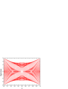
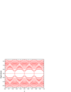
Figure 3: The energy spectrum as function of the magnetic flux for three values of the hopping integral $t^{\prime}$ (see text) : (left) $t^{\prime}=1$, corresponding to the simple square lattice, (middle) $t^{\prime}=0.5$, (right) $t^{\prime}=0$, corresponding to the square lattice with centered lines (Lieb lattice). $\phi$ is the magnetic flux through the unit cell of the simple lattice measured in quantum flux units. The Hofstadter butterfly is obvious for $t^{\prime}=1$, while a doubled butterfly results for $t^{\prime}=0$ in each of the intervals $\phi\in[0,0.25]$, $\phi\in[0.25,0.5]$, etc. (one has to keep in mind that the flux through the Lieb unit cell is four times larger than $\phi$). The energy is measured in units of hopping integral $t$.

III Specific aspects of the finite Lieb plaquette in magnetic field: zero energy flat band and twisted edge states

III.1 The properties of the flat band

There are several pertinent questions which can be asked concerning the flat band in the energy spectrum of the Lieb finite system: what is the degeneracy, what is the response to the magnetic and electric field and to the disorder?

Let us find first the conditions which should be satisfied by the zero energy eigenfunction $\Psi_{E=0}$. Let $H$ be the tight-binding Hamiltonian of a finite system and $\Psi_{E}$ its eigenfunctions:

$$H=\sum_{n}E_{n}|n><n|+\sum_{n,m}t_{nm}|n><m|,~{}~{}\Psi_{E}=\sum_{n}\alpha_{n}|n>,$$ (14)

where $\{|n>\}$ is a basis of functions localized at the sites $n$. The condition $H\Psi_{E}=0$ generates a set of equations for the coefficients $\{\alpha_{n}\}$:

$$E_{n}\alpha_{n}+\sum_{m}t_{nm}\alpha_{m}=0,~{}~{}\forall n.$$ (15)

Eqs.(15) are the necessary and sufficient conditions which must be fulfilled by the wave function $\Psi_{E}$ in order to correspond to the zero eigenvalue $E=0$. With $E_{n}=0$, and taking into account only the nearest neighbors ($t_{nm}=t$) the above equations become simply $\sum_{m\in{\mathcal{V}}_{n}}\alpha_{m}=0$, for any $n$, where the sum is taken over all sites in the first vicinity ${\mathcal{V}}_{n}$ of the site $n$. In addition, if $\Psi^{i}_{E=0}$ and $\Psi^{j}_{E=0}$ are two degenerate states , the orthogonality condition reads $\sum_{n}\alpha^{i}_{n}\alpha^{j}_{n}=0$. The number of configurations $\{\alpha_{n}\}$ which satisfy simultaneously the two conditions equals the dimension of an orthogonal basis in the space of the degenerate eigenfunctions at $E=0$.

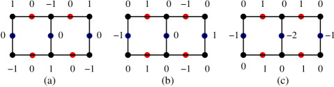
Figure 4: (Color online) The three eigenstates of the flat band for a Lieb lattice composed of two cells. The eigenfunctions are $\Psi^{(0)}=\sum_{nm}\alpha_{nm}|nm>$ and the coefficients $\alpha_{nm}$ are indicated. We notice that the condition for the flat band appearance $\sum_{nm\in{\mathcal{V}}_{n_{0}m_{0}}}\alpha_{nm}=0$ holds for any site $\{n_{0}m_{0}\}$.

An instructive illustration is the Lieb plaquette consisting of two cells (see Fig.4). The plaquette contains 13 atoms (6 of type $A$, 4 of type $B$ and 3 of type $C$). There are three configurations of the coefficients $\alpha_{n}$ which satisfy the conditions discussed above and they are pictured as (a), (b) and (c). (The numbers $\{0,-1,1,-2\}$ mentioned in Fig.4 represent the values, up to the normalization factor, of the coefficients $\alpha_{n}$).

With the notations used in the Hamiltonian (1), the three states can be written as:

$$\Psi^{(0)}_{1}(E=0,\phi=0) = [-a^{\dagger}_{11}+a^{\dagger}_{21}-a^{\dagger}_{22}+a^{\dagger}_{12}-a^{\dagger}_{31}+a^{\dagger}_{32}]~{}|0>$$

$$\Psi^{(0)}_{2}(E=0,\phi=0) = [b^{\dagger}_{11}-b^{\dagger}_{21}-c^{\dagger}_{11}+c^{\dagger}_{31}+b^{\dagger}_{12}-b^{\dagger}_{22}]~{}|0>$$

$$\Psi^{(0)}_{3}(E=0,\phi=0) = [b^{\dagger}_{11}+b^{\dagger}_{21}-c^{\dagger}_{11}-2c^{\dagger}_{21}-c^{\dagger}_{31}+b^{\dagger}_{12}+b^{\dagger}_{22}]~{}|0>$$ (16)

It is obvious that $\sum_{n}\alpha^{i}_{n}=0$ for any $i=1,2,3$ and that $<\Psi_{i}|\Psi_{j}>=0$ for any $i,j=1,2,3$, i.e. the three states correspond to $E=0$ and are mutually orthogonal.

Next, we want to find out how the zero energy states Eq.(16) respond to a perpendicular magnetic field. In order to answer this question, we write the Hamiltonian (1) as:

$$H(\phi) = H^{(0)}(\phi=0)+H^{(1)}(\phi),$$

$$H^{(1)}(\phi) = \sum_{nm}\big{(}a^{\dagger}_{nm}b_{nm}+b^{\dagger}_{nm}a_{n+1,m}\big{)}(e^{-i\pi m\phi}-1)+H.c.,$$ (17)

and perform degenerate perturbation with respect to $H^{(1)}$. Applying this approach to the two-cell Lieb system the matrix elements involved are $<\Psi^{(0)}_{1}|H^{1}|\Psi^{(0)}_{2}>=8i~{}sin\pi\phi$ and $<\Psi^{(0)}_{2}|H^{1}|\Psi^{(0)}_{3}>=0$ and the secular equation reads:

$$\det\left(\begin{array}[]{ccc}-E&8i~{}sin\pi\phi&0\\ -8i~{}sin\pi\phi&-E&0\\ 0&0&-E\end{array}\right)=0,$$

giving rise to the eigenvalues: $E_{1,2}=\pm 8tsin\pi\phi$ and $E_{3}=0$.

One remarks that the bulk state $\Psi_{3}$ does not couple to the magnetic field and its eigenenergy remains $E_{3}=0$. On the other hand, the surface states $\Psi_{1,2}$ get a dispersion which depends on $\phi$. The conclusion of the perturbative calculation is that the magnetic field reduces by 2 the degeneracy of the zero energy band.

Let us generalize now to a finite Lieb lattice containing N cells along the Ox-axis and M cells along Oy-axis, so that the total number of cells is $N_{cell}=NM$ and the number of states is 3NM+2(N+M)+1. It has been proved in the previous chapter that, at zero magnetic field, the number of zero energy degenerate states is $N_{cell}+1$. Then, the two-cell model shows that in the presence of the magnetic field two states separates from the bunch so that the degeneracy of the flat band becomes $N_{cell}-1$. Using a similar approach for the general case, one has to use the eigenfunctions Eq.(11) and Eq.(13) and the expression Eq.(17) as the perturbation. One finds out easily that $<\Phi^{0}(\vec{k})|H^{(1)}\Phi^{0}(\vec{k^{\prime}})>=0$, and that the only nonvanishing matrix elements are $X(\vec{k})=:<\Phi^{0}(\vec{k})|H^{(1)}\Phi^{0}_{a}>$. In the general case, the secular equation becomes:

$$\det\left(\begin{array}[]{ccccc}-E&0&~{}0&...&X(\vec{k}_{1})\\ 0&-E&~{}0&...&X(\vec{k}_{2})\\ ...&...&...&...&...\\ X(\vec{k}_{1})&X(\vec{k}_{2})&~{}X_{3}&~{}~{}...&-E\\ \end{array}\right)=0,$$

which in the polynomial form reads $E^{N-2}(E^{2}-X^{2})=0$, where $X^{2}=X^{2}(\vec{k}_{1})+...X^{2}(\vec{k}_{N-1})$. This formula (where $N$ stands here for the degeneracy of the flat band) says that from the whole bunch only two levels get a dispersion depending on $\phi$, meaning that the degeneracy of the zero energy level is reduced by $2$ in the presence of the magnetic field. So, the general finite Lieb plaquette behaves similarly to the two-cell model.

The numerically calculated energy spectrum of the finite plaquette in perpendicular magnetic field is shown in Fig.5a, where one can check again the presence of the two levels which separates from the flat band while the most of the bunch at $E=0$ consisting of $N_{cell}-1$ states remains dispersionless.

Figure 5: The Hofstadter-type spectrum of a finite Lieb lattice of dimension $N^{x}_{cell}=N^{y}_{cell}=10$. (a) for the clean plaquette, and (b) for the disordered one (disorder strength $W=1$); the flux $\phi$ is measured in quantum flux units.

The strong degeneracy of the flat band can be however lifted by a disordered potential. The broadening of the band depends on the strength of the disorder, however it remains independent of the magnetic field as in the case of the clean system (see Fig.5b). We use a diagonal disorder of the Anderson-type characterized by the width parameter $W$ note1 . The calculation of both the inverse participation number (IPN) and of the interlevel distribution indicate that in the middle of the disordered band the states are still delocalized, and described by the orthogonal Wigner-Dyson distribution ($\beta=1$) which is the typical result in the absence of the magnetic field. This proves once more the absence of response of the flat band to the perpendicularly applied magnetic field, even in the presence of disorder.

The inverse participation number (IPN) is defined as:

$$IPN_{E}=\sum_{n}|<n|\Psi_{E}>|^{4}$$ (18)

and indicates the degree of localization of the states. The small values of the IPN for energies in the middle of the density of states denotes the presence of extended states, and, as expected, the localization increases towards the band edges. The numerically calculated density of states and the dependence on energy of the inverse participation number are shown in Fig.6a. Further information about the localization and the response to the magnetic field is provided by the distribution function of the level spacing between consecutive eigenvalues $s_{n}=E_{n}-E_{n-1}$ of the disordered system. Let us define the dimensionless quantity $t_{n}=s_{n}/<s_{n}>$, where $<s_{n}>$ is the mean level spacing. In the disordered system, in the range of delocalized states, the level spacings are distributed according to the Wigner-Dyson surmise Mehta :

$$\mathcal{P}(t)=b_{\beta}t^{\beta}e^{-a_{\beta}t^{2}},$$ (19)

where $\beta=2$ in the presence of the magnetic field, and $\beta=1$ if $B=0$. As a signature of the distribution, the variance of the level spacing $\delta t=<\delta s>/<s>$ is $<\delta t>=0.4220$ in the first case, and $<\delta t>=0.5227$ in the second one. Fig.6b shows the numerically calculated variance of the level spacing distribution, and one can notice that, in the middle of the flat band, where the states are delocalized, the variance is $<\delta t>=0.5227$. This means that, despite the presence of the magnetic field, the flat band behaves according to the orthogonal ($\beta=1$) Wigner-Dyson distribution instead of the unitary one ($\beta=2$), as it is expected at $B\neq 0$.

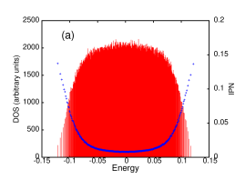
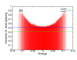
Figure 6: (Color online)(a) The density of states and IPN in the flat band range as function of the energy for a disordered Lieb plaquette of dimension $20\times 20$ cells averaged over 1000 configurations (disorder strength $W=0.3$). (b) The variance of the level spacing distribution as function of energy for the same disordered system; the horizontal lines correspond to 0.4220 (as for the unitary ensemble) and 0.5227 (as for the orthogonal ensemble).

Another way to lift the degeneracy of the zero-energy band is to apply an in-plane static electric field. We expect specific aspects coming from the existence of the edges and of the lattice structure. In the numerical calculation the electric field applied along Oy-axis is simulated by replacing the atomic energies $E_{nm}$ with $E_{nm}+{\mathcal{E}}y_{n}$, where $y_{n}$ is the site coordinate along Oy. Fig.7a shows how the eigenvalues stemming from the flat band are split in several degenerate mini-bands which develop a Stark fan with increasing electric field. It can be checked that the number of mini-bands equals the number of lattice cells along the direction of the electric field. A perpendicular magnetic field gives rise to supplementary fine splitting and to the presence of states between mini-bands. This can be seen in Fig.7b and also in Fig.8. We have noticed that the flat band states are much more sensitive to the electric field than the edge states, and they give rise to a Wannier-Stark ladder at values of the electric field $\mathcal{E}$ for which the edge states are still non affected. We have also numerically observed that the wave function in the $l-th$ miniband is mainly localized in the $l-th$ row of cells in the direction of the electric field.

Figure 7: The low energy spectrum of a finite Lieb plaquette as function of the electric potential applied on the plaquette in the Oy-direction at: (a) $\phi=0$, and (b) $\phi=0.12$.

We already have seen that the flat band states do not show any diamagnetic response, and it is somehow surprising that the Wannier-Stark states coming from the former flat band exhibit a diamgnetic moment when the magnetic field is applied. It is interesting that each mini-band shows both positive and negative magnetic moments, and Fig.8a suggests that the chirality $dE/d\phi$ changes the sign at the center of the mini-band.

Figure 8: The behavior of the flat band in crossed magnetic and electric field. (a) The orbital magnetization $M_{\alpha}$, and (b) the edge localization $P_{\alpha}^{edge}$ (b) vs. energy $E_{\alpha}$ for a finite Lieb lattice of dimension $N^{x}_{cell}=N^{y}_{cell}=15$. The flat band turns into a set of 15 minibands, every miniband being composed of two parts with opposite magnetization. The states in the lowest and highest miniband have significantly increased edge localization ($\phi=0.12$ and $e\mathcal{E}L_{y}=0.2$).

We have studied also the localization properties of the eigenstates, particularly the localization along the edges $P^{edge}_{\alpha}$, defined as:

$$P^{Edge}_{\alpha}=\sum_{i\in Edge}|\Phi_{\alpha}(i)|^{2},$$ (20)

where the index $\alpha$ indicates the state, and the sum is taken over all the sites which belong to the plaquette boundary. It turns out that the states which belong to the mini-bands from the extremities of the fan spectrum are strongly localized along the edges (Fig.8b). The localization is of electric origin since the picture is similar no matter whether the magnetic field is present or not.

We conclude, saying that the disorder lifts the degeneracy of the flat band keeping the states independent of the magnetic field, while the electric field produces states which respond to the magnetic field and show specific diamagnetic moments.

III.2 The twisted and type II edge states and their properties

The confinement of the Lieb lattice induces several types of edge states. Besides the conventional edge states found in the Bloch-Landau and Dirac-Landau regions, there are still two other classes of edge states. We discuss first the twisted edge states lying in the magnetic gap opened around the degenerated energy level $E=0$. Although the new states are localized along the perimeter of the plaquette, they do not follow the known behavior of the conventional edge states. The new class of edge states manifest specific properties: i) their energy depends on the flux in a periodic way. This means that the chirality defined by the sign of $dE/d\phi$ is not conserved but alternate when changing the flux, in contradistinction to the usual edge states either in the Bloch-Landau or Dirac-Landau domain. Obviously, the alternate chirality should be reflected also in oscillations of the orbital magnetization at the variation of the magnetic flux. ii) their energies as function of the flux appear as twisted into bunches; for the clean square plaquette shown in Fig.9a each bunch consists of four states. iii) the states prove the lack of robustness against disorder and iv) prove specific transport properties, namely, the twisted edge states carry a finite longitudinal resistance accompanied by vanishing Hall resistance.

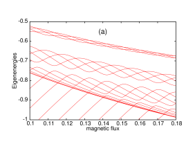
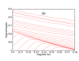
Figure 9: The eigenenergy in the range of the twisted edge states vs. the magnetic flux $\phi$ for a pure Lieb lattice (a) and for a disorder Lieb lattice (b). The twisted edge states has an oscillatory behavior when the magnetic flux is varied, and they form bunches with four states in each bunch. The oscillatory behavior is destroyed by disorder in the right figure, but the conventional edge states (shown in the lower part of the spectrum) remain robust against disorder. The dimension of the Lieb lattice is $N^{x}_{cell}=N^{y}_{cell}=10$ and the amplitude of the Anderson disorder is $W$=1.

A piece of the spectrum of the clean plaquette in the energy range of twisted edge states is shown in Fig.9a, where bunches consisting of four twisted edge states can be observed. One also has to notice that, at a given flux, the states in the bunch may show opposite chirality meaning that they carry diamagnetic currents moving in opposite directions. In the presence of disorder (Fig.9b) one notices that the twisted eigenenergies get stretched but the rest of the spectrum (the band and the edge states in the Dirac region) is not affected. This indicates that the twisted states are very sensitive to disorder. The understanding of this effect is simple in the sense that the degeneracy at crossing points note2 is lifted by the perturbation introduced by the impurity potential, and this occurs even at weak disorder.

Figure 10: The behavior of the edge states with disorder. (a) The absence of the backscattering for a conventional edge states. A pair of twisted states which are sufficiently close in energy may suffer the backscattering suggested in (b), which induces the localization shown in Fig.11.

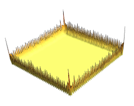
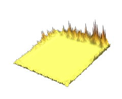
Figure 11: $|\Psi|^{2}$ calculated for a conventional edge state in the Dirac range (left) and for a twisted edge state (right) for a disordered plaquette with $W=0.2$. One observes that this low disorder does not affect the conventional edge state but localizes the twisted state.

Figure 12: The eigenenergies vs. the magnetic flux $\phi$ for a pure Lieb lattice in the range which emphasizes the type II edge states. In the spectrum, they are located between the bulk states in the Dirac-Landau range and the conventional edge states of the first gap. Their energy decreases with the magnetic field similar to the bulk states, however they have edge localization of the wave function. The dimension of the Lieb lattice is $N^{x}_{cell}=N^{y}_{cell}=10$.

The Lieb lattice exhibits still another specific edge states (which we call type-II edge states), which in Fig.12 are placed immediately above the Dirac-Landau bands at the transition from Dirac bulk to conventional edge states. They cannot be identified according to the sign of the magnetic moment Nita since their chirality $dE_{n}/d\phi$ is the same as for the bulk (band) states note3 .

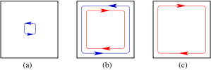
Figure 13: The sketch of the diamagnetic currents in the Dirac-Landau range of the spectrum: (a) the counterclockwise loop of a bulk state, (b) the double ridge current of a type-II edge states, and (c) the clockwise loop of a conventional edge states. The twisted edge states may show both (b) and (c) aspect.

Nevertheless, the diamagnetic currents of these states are located along the edges of the plaquette. These edge states show a double-ridge profile and carry current in both directions, but nonetheless the total magnetization remains of bulk-type.

In Fig.13 the diamagnetic currents of bulk states, type-II edge states and of conventional edge states are sketched. The twisted edge states may show currents similar to both conventional and type-II edge states. Compared to the twisted states, the type-II edge states behave substantially different in the electronic transport. These states will be studied in detail elsewhere.

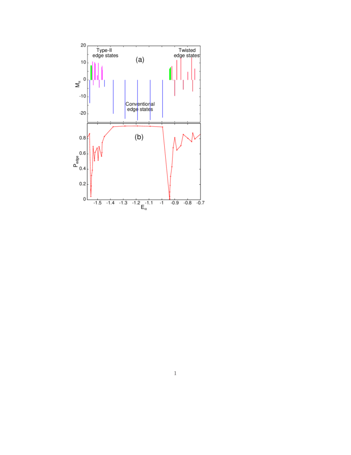
Figure 14: (Color online) Magnetization $M_{\alpha}$ and localization at the edges $P_{edge}$ corresponding to the eigenenergies $E_{\alpha}$: the bulk (band) states (green) show positive magnetization and vanishing localization at the edges; the conventional edge states (blue) show negative magnetization and $97\%$ localization at the edges; the type-II and the twisted states show $60-80\%$ localization at the edges. The data are for a clean Lieb plaquette of dimension $N_{cell}^{x}=N_{cell}^{y}=10$ and $\phi=0.16$.

The contribution to the magnetization of each eigenstates $|\alpha>$ is calculated following the approach from Aldea-magn , namely:

$$M_{\alpha}= -<\alpha|\frac{dH}{d\phi}|\alpha>$$

$$= i\pi t_{x}\sum_{mn}\big{(}me^{-im\pi\phi}<\alpha|A_{nm}><B_{nm}|\alpha>-me^{im\pi\phi}<\alpha|A_{nm}><B_{n-1,m}|\alpha>$$

$$+ me^{-im\pi\phi}<\alpha|B_{nm}><A_{n+1,m}|\alpha>-me^{im\pi\phi}<\alpha|B_{nm}><A_{nm}|\alpha>\big{)}.$$ (21)

All the matrix elements in the above equation are known once the eigenstates $|\alpha>$ are calculated numerically in the presence of the magnetic flux. Fig.14 depicts the diamagnetic moments and the localization at the edges of different type of states. The bulk (band) states show positive magnetization and vanishing localization at the edge, the conventional edge states show negative magnetization, and $97\%$ localization at the edge. The twisted edge states show alternating magnetization, as expected, but also an unanticipated differences in the degree of edge localization. This is because they exhibit either a single- or double-ridge wave function. Obviously, the double-ridge wave function is not strictly stuck to the edge so that $P_{edge}\approx 0.7-0.8$, while for the single-ridge states the same parameter goes up to $0.9$. Fig.14 points out that the single-ridge states which are localized close to the edge exhibits negative magnetization (as the conventional edge states), while the double-ridge states exhibits positive magnetization.

IV The integer quantum Hall effect

The quantum transport of the 2D Lieb plaquette shows some similarities with the case of graphene, however it also reveals particular properties. The Hall resistance as function of the Fermi energy at a given quantizing magnetic field was obtained in Ref.3 by calculating the Chern numbers, and has the general aspect which can be observed in Fig.15 which we obtain in the Landauer-Büttiker formalism: starting from the bottom of the spectrum, $R_{H}$ shows $h/e^{2}$ steps in the Bloch-Landau region, then change the sign, and shows again $h/e^{2}$ steps in the Dirac-Landau region. The steps of the quantum Hall plateaus differs from those of the honeycomb lattice since in the Lieb case there is only one Dirac cone per the unit cell. The change of sign is associated with the opposite chirality of the edge states in the two regions and occurs at $E=\pm 2t$, while in graphene the same change takes place at $E=\pm t$ graph . The density of states (shown in blue in Fig.15) is calculated as $DOS=-\frac{1}{\pi}\sum_{n}ImG^{+}_{nn}(E)$, where $G^{+}$ is the retarded Green function for the mesoscopic plaquette connected to the leads. In order to calculate the transport properties the mesoscopic plaquette must be connected to leads, the whole system being described in the tight-binding approach by the Hamiltonian:

$$H=H^{S}+H^{L}+\tau H^{LS},$$ (22)

where the first term is just the Hamiltonian (1), the second term describes all the leads, and $H^{LS}$ couples the leads to the plaquette with the strength $\tau$. With $G^{+}_{\alpha,\beta}(E)\equiv<\alpha|(E-H+i0)^{-1}|\beta>$, the electron transmittance between the leads $\alpha$ and $\beta$, in the Landauer-Büttiker formalism, is given by:

$$T_{\alpha,\beta}=4\tau^{4}|G^{+}_{\alpha,\beta}(E_{F})|^{2}Img^{L}_{\alpha}(E_{F})Img^{L}_{\beta}(E_{F}),$$ (23)

where $g^{L}$ is the Green function of the isolated leads.

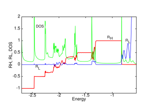
Figure 15: (Color online) The transport properties of the Lieb lattice under the magnetic field: Hall resistance $R_{H}$, longitudinal resistance $R_{L}$ and density of states DOS for a finite Lieb lattice connected to four transport leads. The quantum Hall effect can be observed for $E\in[-2.75,-0.8]$ ($R_{H}$ integer and $R_{L}=0$). In the Bloch-Landau part of the spectrum ($E<-2$) one has $R_{H}<0$, while in the Dirac-Landau part ($E>-2$) one has $R_{H}>0$. In the energy range $E\in[-0.8,-0.6]$ the transport properties are due to the twisted edge states and we get zero Hall resistance $R_{H}=0$ and oscillations of the longitudinal resistance with the characteristic minima at $R_{L}=1/4$. The density of states exhibits maxima at the transition between the Hall plateaus and for the energy values where the twisted edge states appear. The dimension of the plaquette is $10\times 30$ unit cells, the magnetic flux is $\phi=0.12$. The resistance is in units $h/e^{2}$, DOS in arbitrary units, and the energy in units $t$.

In what follows we shall discuss the interesting question of the contribution to transport of the twisted edge states introduced in the previous section. The answer can be found in Fig.15 in the energy range $E\in[-0.8,-0.6]$, where one observes that the twisted edge states found in that range do not support the Hall resistance ($R_{H}=0$), however they contribute to the longitudinal resistance, which exhibits an oscillating behavior. It is also to notice that all the oscillations minima equals $R_{L}=1/4$, a fact that should find its explanation.

In exploring these unexpected effects, the first step should be to identify the transmittance matrix. The numerical investigation presented in Fig.17a shows that, in the range of the twisted edge states the properties of transmittances $T_{\alpha,\beta}$ are very specific: they are not quantized, show an oscillating dependence on the energy, and, mainly, satisfy the symmetry relation:

$$T_{\alpha,\alpha+1}=T_{\alpha+1,\alpha},$$ (24)

while in the range of the conventional edge states, where the quantized plateaus occur, the usual properties of quantum Hall effect hold: $T_{\alpha,\alpha+1}$=integer and $T_{\alpha+1,\alpha}=0$ (for a given sign of the magnetic flux).

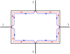
Figure 16: (Color online) The four-lead Hall device: illustration of the edge currents carried by the twisted edge states, for which the symmetry relation $T_{\alpha,\alpha+1}=T_{\alpha+1,\alpha}$ holds.

Combining Eq.(24) with the general property $\sum_{\alpha}T_{\alpha,\beta}=0$, which expresses the current conservation, it turns out that the transmittance matrix for the edge transport in the domain of twisted edge states can be written as:

$$\mathcal{T}=\left(\begin{array}[]{cccc}-2T&T&0&T\\ T&-2T&T&0\\ 0&T&-2T&T\\ T&0&T&-2T\\ \end{array}\right).\hskip 28.45274pt$$

The transmittance $T_{\alpha,\beta}$ relates the current through the lead $\alpha$ to potentials at the contact sites $\beta$ as:

$$I_{\alpha}=\frac{e^{2}}{h}\sum_{\beta}T_{\alpha\beta}V_{\beta},$$ (25)

and, for the four-lead device considered in Fig.16, in the Landauer-Büttiker formalism, the Hall and longitudinal resistance are given (in units $h/e^{2}$) by:

$$R_{L} = R_{14,23}=(T_{24}T_{31}-T_{21}T_{34})/D,$$

$$R_{H} = (R_{13,24}-R_{24,13})/2=(T_{23}T_{41}-T_{21}T_{43}-T_{32}T_{14}+T_{12}T_{34})/2D,$$ (26)

where $D=-4T^{3}$ is a subdeterminant of the matrix $\mathcal{T}$. By the use of the above equations and of transmittance matrix $\mathcal{T}$, valid in the range of twisted edge states, one obtains immediately, a vanishing Hall resistance ($R_{H}=0$) and the longitudinal resistance $R_{L}=1/4T$ (in units $h/e^{2}$). The minima of $R_{L}$ observed in Fig.17b correspond to the maxima of the transmittance, and, obviously, the value $R_{L}=0.25h/e^{2}$ expresses a perfect conducting one channel transport with $T=1$. It turns out that, although carried by edge states, the current shows a dissipative character.

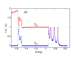
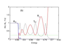
Figure 17: (Color online) (a) The transmittances $T_{12}$ and $T_{21}$ showing the quantized values $T_{12}=1$ and $T_{21}=0$ in the range of the IQHE, non-quantized oscillating values $T_{12}=T_{21}$ in the range of twisted edge states $E>-0.95$, and $T_{12}=T_{21}+1$ in the range of type-II edge states $E\in[-1.55,-1.5]$. (b) The Hall and longitudinal resistance: $R_{H}$ (blue line) vanishes in the range of twisted edge states, while $R_{L}$ (red line) exhibits oscillations with minima $R_{L}=0.25$. The minima of the longitudinal resistance occur at the energies where the transmittance (black dashed line) get the maximum value $T_{12}=T_{21}=1$. The dimension of the plaquette is $10\times 30$ unit cells, $\phi=0.16$.

The oscillations of $T_{12}$ and $T_{21}$ in the domain of the twisted edge states ($E\in[-0.95,-0.75]$) follow the similar oscillations of the density of states, while in the quantum Hall regime (E $\in$ [-1.5,-0.95]) the DOS is flat.

Another interesting problem is the transition between the first and second plateau of the Dirac-Landau region ($E\in[-1.55,-1.5]$) which is much wider than similar transitions in the Bloch-Landau region. The transition get a width which is due to the presence of the type-II edge states (observed in the spectrum Fig.12 above the Dirac band), and is accompanied by oscillations of the transmittance (see $T_{12}$ and $T_{21}$ in Fig.17a). We have to stress that in this energy range $T_{12}$ and $T_{21}$ are no more equal, and the numerical calculation suggests that $T_{12}=T_{21}+1$. It means that the symmetry Eq.(24) remains specific to the twisted edge states.

In order to figure out a scenario for the vanishing Hall effect, we remind first that, in the range of the QH effect, all the (conventional) edge states responsible for the plateaus of the transverse magnetoresistance get a unique chirality determined by the direction of the magnetic flux. This results in a definite sense (say clock-wise) of the current such that $T_{\alpha,\alpha+1}$= integer and $T_{\alpha+1,\alpha}=0$. The symmetry $T_{\alpha,\alpha+1}=T_{\alpha+1,\alpha}$ which occurs in the range of the twisted edge states is characteristic to the absence of the magnetic field. So, this symmetry indicates a ’loss of influence’ of the magnetic field followed by a vanishing Hall effect. As a support of this idea we note that the twisted edge states show alternating (clock and anti-clock) chiralities which allow for the transmittance in both directions, as sketched in Fig 16. This might be an heuristic explanation for the vanishing of the transverse resistance despite the presence of edge states.

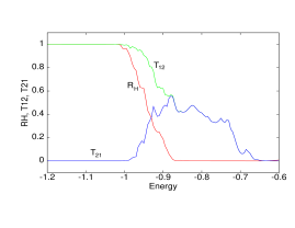
Figure 18: (Color online) The Hall resistance $R_{H}$ (red) and transmittances $T_{12}$ (green) and $T_{21}$ (blue) for a disordered Lieb lattice in the transition region from the first Hall plateau to the domain of twisted edge states. The figure shows that the symmetry relation $T_{12}=T_{21}$ for twisted edge state transport holds also in the presence of disorder. The Hall resistance is $R_{H}=1$ for the energies corresponding to the first gap with conventional edge states, and $R_{H}=0$ for the energies corresponding to the twisted edge states. The dimension of the plaquette and the magnetic flux are the same as in Fig.17, the disorder amplitude is $W=0.5$.

Let us discuss now the effect of the disorder. It is known that the conventional edge states are robust to disorder, whereas the bulk states (which form the Landau bands) are more sensitive, so that the IQHE of a disordered plaquette shows robust plateaus, and a broadened transition region between two consecutive plateaus. On the other hand, as we have shown, the disorder localizes easily the twisted edge states, changing in this way their transmittance properties. Fig.18 depicts the transmittances $T_{12},T_{21}$ for a disordered Lieb plaquette compared to the same transmittances of the clean system. One observes the quantized values in the range of the conventional edge states followed, in the range of twisted states, by reduced values of the disordered transmittance which replace the peaks specific to the clean system. It is worth to say that the symmetry $T_{\alpha,\alpha+1}=T_{\alpha+1,\alpha}$ is preserved for each individual disordered sample, and, as a consequence, the Hall effect vanishes similar to the clean case.

V Conclusions

We have found that the specific topology of the 2D Lieb lattice induces remarkable spectral and transport properties. Up to point there are similarities with the electronic energy spectrum of graphene in what concerns the presence of a Dirac-type cone at low energy, however, in addition, a macroscopically degenerated flat band occurs at the middle of the spectrum. The perpendicular magnetic field applied on a finite (mesoscopic) Lieb plaquette opens a gap around the flat band, and we show the presence in this gap of a new class of edge states with alternating chirality (which we call twisted edge states). The flat band is insensitive to the magnetic field, however an in-plane electric field, and also the disorder, lifts the degeneracy. The electric field applied on a finite (mesoscopic) system gives rise to a Wannier-Stark fan composed of degenerate mini-bands, the number of them being equal to the number of cells along the direction of the field.

The macroscopic degeneracy of the flat band is lifted by disorder, and the degree of localization and the level spacing distribution are studied. It turns out that not only the ordered flat band, but also the disordered one, does not feel the magnetic field; indeed, we prove that the level spacing distribution of the disordered system follows the orthogonal ($\beta=1$) Wigner-Dyson distribution, which usually describes disordered systems in the absence of the magnetic field.

We calculate analytically the orthogonal eigenfunctions of the finite Lieb system corresponding to the three spectral branches in the low energy range, both for periodic and vanishing boundary conditions. In this way we find also the degeneracy of the zero energy flat band which, in the periodic case, equals the total number of unit cells $N_{cell}$ (except when both $N^{x}_{cell}$ and $N^{y}_{cell}$ are even numbers, in which case the degeneracy increases to $N_{cell}+2$), while in the case of the closed boundaries the degeneracy is $N_{cell}+1$. A toy model composed of only two unit cells helps to understand the behavior in the presence of a perpendicular magnetic field. The perturbative calculation shows that 2 states of the flat band separate from the degenerated bunch, and belong to the class of twisted edge states.

The eigenenergies of the twisted edge states depend in an oscillatory manner on the magnetic flux, i.e., show an alternating chirality, and contrary to the conventional edge states, the diamagnetic moment change the sign when the magnetic flux is varied. These type of edge states generated by the magnetic field are not protected by the broken time-reversal symmetry, and proves to get localized even at low disorder, when the conventional edge states remain robust.

The transport properties are calculated by attaching leads to the finite Lieb system and using the Landauer-Büttiker formalism. The quantum Hall resistance looks similar to that of the graphene except the steps are equal to $h/e^{2}$ (instead of $h/2e^{2}$), however in the domain of the twisted edge states the properties become unconventional: the Hall resistance vanishes, while the longitudinal one shows oscillations which can be correlated with the oscillations of the density of states (calculated in the presence of the leads). This behavior stems from the symmetry of the transmittance $T_{\alpha,\alpha+1}=T_{\alpha+1,\alpha}$ which occurs despite the presence of the quantizing magnetic field. The symmetry holds also in the presence of disorder.

VI Acknowledgements

We acknowledge support from PNII-ID-PCE Research Programme (grant no 0091/2011), Core Programme (contract no.45N/2009) and Sonderforschungsbereich 608 at the Institute of Theoretical Physics, University of Cologne. One of the authors (AA) is very much indebted to A.Rosch for illuminating discussions.

References

- (1) R. Rammal, J. Physique 46, 1345 (1985).
- (2) H. Aoki, M. Ando, and H. Matsumura, Phys. Rev. B 54, R17296 (1996).
- (3) N. Goldman, D. F. Urban and D. Bercioux, Phys. Rev A 83, 063601 (2011).
- (4) R. Shen, L. B. Shao, B. Wang, and D. Y. Xing, Phys. Rev. B 81, 041410(R)(2010).
- (5) C. Weeks and M. Franz, Phys. Rev. B 82, 085310 (2010).
- (6) W. Beugeling, J. C. Everts, and C. Morais Smith, Phys. Rev. B 86, 195129 (2012).
- (7) W. F. Tsai, C. Fang, H. Yao, J. Hu, e-print arXiv:1112.5789.
- (8) Y. F. Wang, H. Yao, Z. C. Gu, C. D. Gong, and D. N. Sheng, Phys. Rev. Lett. 108, 126805 (2012).
- (9) S. Yang, K. Sun and S. DasSarma, Phys. Rev. B 85, 205124 (2012).
- (10) M. Trescher and E. J. Bergholtz, e-print arXiv:1205.2245.
- (11) W. Zhang, e-print arXiv:1201.0722.
- (12) A. Zhao and S. Q. Shen, Phys. Rev. B 85, 085209 (2012).
- (13) N. B. Kopnin, T. T. Heikkila, and G. E. Volovik, Phys. Rev. B 83, 220503(R) (2011).
- (14) E. H. Lieb, Phys. Rev. Lett. 62, 1201 (1989).
- (15) V. Apaja, M. Hyrkas, and M. Manninen, Phys. Rev. A 82, 041402(R) (2010).
- (16) This is to be expected since also the corresponding Landau bands show opposite chirality.
- (17) The energy in the Hamiltonian (1) is a random variable described by the distribution for , and zero otherwise.
- (18) M. L. Mehta, Random Matrices and Statistical Theory of Energy Levels (Academic, New York, 1967).
- (19) The degeneracy at the apparent crossing points could be shown only numerically; by reducing progressively the grid down to (in units ) the distance between the consecutive eigenvalues decreases progressively to (in units ).
- (20) M. Niţă, A. Aldea and J.Zittartz, Phys. Rev. B 62, 15367 (2000).
- (21) A. Aldea, V. Moldoveanu, M. Niţă, A. Manolescu, V. Gudmundsson, and B. Tanatar, Phys. Rev. B 67, 035324 (2003).
- (22) D. N. Sheng, L. Sheng, and Z. Y. Weng, Phys. Rev B 73, 233406 (2006).