Spectral function of the Bloch-Nordsieck model at finite temperature

Abstract

In this paper we determine the exact fermionic spectral function of the Bloch-Nordsieck model at finite temperature. Analytic results are presented for some special parameters, for other values we have numerical results. The spectral function is finite and normalizable for any nonzero temperature values. The real time dependence of the retarded Green’s function is power-like for small times and exhibits exponential damping for large times. Treating the temperature as an infrared regulator, we can also give a safe interpretation of the zero temperature result.

I Introduction

The behavior of the ultra-soft regime of massless field theories presents a serious challenge which, on the other hand, is crucial for understanding of the most, physically relevant theories. The soft nature of the excitations perturbatively leads to infrared (IR) divergences in various physical quantities such as the self-energy near the mass shell. To have reliable results, one has to resum the most sensitive part of the IR physics. The identification of the sources of these divergences, the elaboration of the appropriate mathematical tools and finally the realisation of the resummation itself is a formidable task. Moreover, the details can depend on the environment, that is the resummation in deep inelastic scattering and at finite temperature equilibrium may require different approaches. It is not a surprise, therefore, that so many resummation methods exist, working at different circumstances.

In this sensitive field, where the physical reliability of a resummation may crucially depend on the correct identification of the relevant sources of the IR divergences, it is quite valuable to find a model which is physically motivated and exactly solvable. This is the reason why so many two-dimensional conformal and integrable theories have relevance. In four dimensions, however, exactly solvable models are much rarer.

A physically well-motivated model is the Bloch-Nordsieck (BN) model BN . In its long history it became a text-book material BogoljubovShirkov ; Fried . Physically it corresponds to the deep IR limit of QED, where the photons have no energy even for a fermion spin-flip. In particular it can be used to prove QED theorems in this energy regime Weldon:1991eg . The BN model can be solved exactly, the photon contributions can be fully summed up. The fermion propagator has been calculated at zero temperature both based on functional methods BogoljubovShirkov ; Fried , and with help of Dyson-Schwinger equations Alekseev:1982dk ; Jakovac:2011aa , where also a detailed renormalization analysis is possible. The spectral function of the model at zero temperature reads in Feynman gauge as

$$\varrho(w,T=0)\sim w^{-1-\frac{\alpha}{\pi}},\qquad\mathrm{where}\quad w=u_{\mu}p^{\mu}-m,\quad\alpha=\frac{e^{2}}{4\pi}.$$ (1)

Here $u$ is a 4-vector parameter of the model, loosely identifiable with the four-velocity of the fermion. This function, however, has a singular behavior: it is not normalizable, therefore the sum rule $\int\rho=2\pi$ can be satisfied only with zero wave function renormalization factor. Moreover, the naive inverse Fourier transform of this function is $\sim t^{\alpha/\pi}$ describing growth of correlation in time. The correct physical interpretation of these results requires some IR regulator, which can be, for example, the temperature.

At finite temperature the model is much less studied. In the seminal papers of Blaizot and Iancu IancuBlaizot1 ; IancuBlaizot2 the authors studied the large time behavior of the fermion propagator with the Hard Thermal Loop (HTL) improved photon propagator. Using this result, Weldon worked out a spectral function which is valid in the vicinity of the mass shell Weldon:2003wp . With a different approach, Fried et. al. studied the time dependence of the momentum loss of a hard incoming fermionic particle Fried:2008tb .

We have several goals in this paper. The main goal is to work out the complete spectral function of the BN model for all momenta, and see how the short time dynamics, resembling the $T\to 0$ limit, goes over to the long time damping. Because of the relative simplicity of the model we can even give analytic solutions for certain parameters, while for other, analytically not reachable parameter values we used a well controlled numerical procedure. Another goal is to extend our Dyson-Schwinger formalism combined with Ward identities Jakovac:2011aa , which works excellently at zero temperature, to finite temperatures. With the help of it, the complete renormalization process remains fully controlled.

Our paper will be organized as follows. First, we define the Bloch-Nordsieck model in Section II. We review the Dyson-Schwinger equations and Ward identities in finite temperature real time formalism, and apply them to the Bloch-Nordsieck model. In Section III we solve these equations. At zero velocity (Subsection III.3) we provide an analytic formula for the fermion propagator, supported by a numerical verification. At nonzero velocity (Subsection III.4) we solve them numerically. In Subsection III.5 we compare our results with previous works in the literature. In Section IV we give the conclusions of the paper.

II The Bloch Nordsieck model at finite temperature

The Bloch-Nordsieck model is the low energy limit of QED, where we take into account only a single spin orientation. Its Lagrangian is related to the QED Lagrangian by changing the Dirac matrices $\gamma^{\mu}$ for a four-vector $u^{\mu}$:

$${\cal L}=-\frac{1}{4}F_{\mu\nu}F^{\mu\nu}+\Psi^{\dagger}(iu_{\mu}D^{\mu}-m)\Psi,\qquad iD_{\mu}=i\partial_{\mu}-eA_{\mu},\quad F_{\mu\nu}=\partial_{\mu}A_{\nu}-\partial_{\nu}A_{\mu}.$$ (2)

We can choose $u$ to be a four-velocity, or it can be $u=(1,\mathbf{v})$: the two are related by a simple field and mass rescaling, since by replacing $\Psi\to\Psi/\sqrt{u_{0}}$ and $m\to mu_{0}$, we can reach the $u_{0}=1$ scenario. The quantity $\mathbf{v}=\mathbf{u}/u_{0}$ can be interpreted as the velocity of the fermion.

We are interested in the finite temperature fermion propagator. To determine it, we use the real time formalism (for details, see LeBellac ). Here the time variable runs over a contour containing forward and backward running sections ($C_{1}$ and $C_{2}$). The propagators are subject to boundary conditions which can be expressed as the KMS (Kubo-Martin-Schwinger) relations. The physical time can be expressed through the contour time $t={\cal T}(\tau)$. This makes possible to work with fields living on a definite branch of the contour, $\Psi_{a}(t,{\bf x})=\Psi(\tau_{a},{\bf x})$ where ${\cal T}(\tau_{a})=t$, and $\tau_{a}\in C_{a}$ for $a=1,2$; and similarly for the gauge fields. The propagators are matrices in this notation:

$$i{\cal G}_{ab}(x)=\left\langle{T_{C}\Psi_{a}(x)\Psi_{b}^{\dagger}(0)}\right\rangle\qquad\mathrm{and}\qquad iG_{\mu\nu,ab}(x)=\left\langle{T_{C}A_{\mu a}(x)A_{\nu b}(0)}\right\rangle,$$ (3)

where $T_{C}$ denotes ordering with respect to the contour variable (contour time ordering). $G_{11}$ corresponds to the Feynman propagator, and, since the $C_{2}$ contour times are always larger than the $C_{1}$ contour times, $G_{21}=G^{>}$ and $G_{12}=G^{<}$ are the Wightman functions. The KMS relation for a bosonic/fermionic propagator reads $G_{12}(t,{\bf x})=\pm G_{21}(t-i\beta,{\bf x})$ which has the following solution in Fourier space

$$iG_{12}(k)=\pm n_{\pm}(k_{0})\varrho(k),\qquad iG_{21}(k)=(1\pm n_{\pm})(k_{0})\varrho(k),$$ (4)

where

$$n_{\pm}(k_{0})=\frac{1}{e^{\beta k_{0}}\mp 1}\quad\mathrm{and}\quad\varrho(k)=iG_{21}(k)-iG_{12}(k)$$ (5)

are the distribution functions (Bose-Einstein (+) and Fermi-Dirac (-) statistics), and the spectral function, respectively. It is sometimes advantageous to change to the R/A formalism with field assignment $\Psi_{1,2}=\Psi_{r}\pm\Psi_{a}/2$. Then one has $G_{aa}=0$ for both the fermion and the photon propagators. The relation between the $1\,2$ and the R/A propagators reads

$$G_{rr}=\frac{G_{21}+G_{12}}{2},\quad G_{11}=G_{ra}+G_{12},\quad\varrho=iG_{ra}-iG_{ar}.$$ (6)

The $G_{ra}$ propagator is the retarded, the $G_{ar}$ is the advanced propagator, $G_{rr}$ is usually called the Keldysh propagator.

At zero temperature the fermionic Feynman-propagator reads:

$${\cal G}_{0}(p)=\frac{1}{u_{\mu}p^{\mu}-m+i\varepsilon}.$$ (7)

It has a single pole which means that there is no antiparticles in the model. Consequently, all closed fermion loops are zero, thus there is no self-energy correction to the photon propagator at zero temperature. Physically this means that the energy is not enough to excite the antiparticles. In fact, if we interpret the $u$ parameter as the four-velocity of the fermion, the Bloch-Nordsieck model describes that regime where the soft photon fields do not have energy even for changing the velocity of the fermion (no fermion recoil). This leads to the interpretation that the fermion is a hard probe of the soft photon fields, and as such it is not part of the thermal medium IancuBlaizot2 . So we will set ${\cal G}_{12}=0$, therefore the closed fermion loops as well as the photon self energy remain zero even at finite temperature. Another, mathematical reason, why we must not consider dynamical fermions – which could show up in fermion loops – is that the spin-statistics theorem PeshkinSchroeder forbids a one-component dynamical fermion field.

This means that now the exact photon propagator reads in Feynman gauge

$$G_{ab,\mu\nu}(k)=-g_{\mu\nu}G_{ab}(k),\qquad G_{ra}=\frac{1}{k^{2}}\biggr{|}_{k_{0}\to k_{0}+i\varepsilon},\quad\varrho(k)=2\pi\mathop{\textrm{sgn}}(k_{0})\delta(k^{2}),$$ (8)

all other propagators can be expressed using identities (4) and (6).

II.1 Dyson-Schwinger equations

The operator equations of motion give relations of the different Green’s functions, formulated as the Dyson-Schwinger equations. These equations are local, and so they are valid in generic non-equilibrium situations, and, of course, in a thermal medium, too.

The generating form of the Dyson-Schwinger equations for generic fields $\Phi_{i}$ reads Collins

$$\left\langle{\frac{\delta S}{\delta\Phi_{i}(y)}\Phi_{a_{1}}(x_{1})\dots\Phi_{a_{n}}(x_{n})}\right\rangle=i\sum\limits_{k=1}^{n}\delta_{ia_{k}}\delta(y-x_{k})\left\langle{\Phi_{a_{1}}(x_{1})\dots\Phi_{a_{k-1}}(x_{k-1})\Phi_{a_{k+1}}(x_{k+1})\dots\Phi_{a_{n}}(x_{n})}\right\rangle.$$ (9)

In real time formalism the time variable is the contour time (usually it is the variable of the path integral). We define the fermionic self energy in the usual way

$${\cal G}(x,y)={\cal G}^{(0)}(x,y)+\int_{C}\!d^{4}x^{\prime}d^{4}y^{\prime}\,{\cal G}^{(0)}(x,x^{\prime})\Sigma(x^{\prime},y^{\prime}){\cal G}(y^{\prime},y),$$ (10)

where the symbol $\int_{C}$ means time integration over the contour. Then we find in the Bloch-Nordsieck model

$$\Sigma(x,y)=i\alpha(x_{0})e^{2}u_{\mu}\int_{C}\!d^{4}wd^{4}z\,{\cal G}(x,w)G^{\mu\nu}(x,z)\Gamma_{\nu}(z;w,y),$$ (11)

where the tree level vertex is $eu_{\mu}$, the proper vertex is denoted by $e\Gamma_{\mu}$, and $\alpha(x_{0})$ is 1 if $x_{0}\in C_{1}$ and $-1$ if $x_{0}\in C_{2}$. This factor appears because we expressed the functional derivative $\frac{\delta S}{\delta\Phi_{i}(y)}$ through the derivatives of the Lagrangian, which, however, changes sign on $C_{2}$.

We can also express this equation with the two-component notation as it can be seen on Fig. 1.

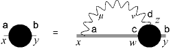
Figure 1: The Dyson-Schwinger equations in real time formalism

In terms of analytic formulas it reads:

$$\Sigma_{ab}(x,y)=i\alpha_{a}e^{2}u_{\mu}\sum_{c,d=1}^{2}\int\!d^{4}wd^{4}z\,{\cal G}_{ac}(x,w)G^{\mu\nu}_{ad}(x,z)\Gamma_{\nu;dcb}(z;w,y),$$ (12)

where $\alpha_{a}=(-1)^{a+1}$. In Fourier space it reads:

$$\Sigma_{ab}(p)=i\alpha_{a}e^{2}u_{\mu}\sum_{c,d=1}^{2}{\int\!\frac{d^{4}k}{(2\pi)^{4}}\,}{\cal G}_{ac}(p-k)G^{\mu\nu}_{ad}(k)\Gamma_{\nu;dcb}(k;p-k,p).$$ (13)

II.2 The vertex function in the Bloch-Nordsieck model

The second use of the Dyson-Schwinger equation is to have a form for the vertex function. From (9) we find for any gauge theories

$$\left\langle{\frac{\delta S}{\delta A^{\mu}(x)}O(\bar{\Psi},\Psi)}\right\rangle=0,$$ (14)

where $O$ is any local operator containing $\bar{\Psi}$ and $\Psi$. This implies, in particular

$$\left\langle{A_{\mu}(x)\Psi(y)\bar{\Psi}(z)}\right\rangle=\int_{C}d^{4}x^{\prime}G_{\mu\nu}(x,x^{\prime})\left\langle{j^{\nu}(x^{\prime})\Psi(y)\bar{\Psi}(z)}\right\rangle,$$ (15)

where $j_{\mu}$ is the conserved current. The vertex function shows up in the $A\Psi\Psi^{\dagger}$ correlator as

$$\left\langle{A_{\mu}(x)\Psi(y)\bar{\Psi}(z)}\right\rangle=\int_{C}\!d^{4}x^{\prime}d^{4}y^{\prime}d^{4}z^{\prime}\,iG_{\mu\nu}(x,x^{\prime})i{\cal G}(y,y^{\prime})(-ie)\Gamma^{\nu}(x^{\prime},y^{\prime},z^{\prime})i{\cal G}(z^{\prime},z).$$ (16)

From here we find

$$\int_{C}d^{4}y^{\prime}d^{4}z^{\prime}\,i{\cal G}(y,u)\,e\Gamma^{\mu}(x;u,v)i{\cal G}(v,z)=\left\langle{j^{\mu}(x)\Psi(y)\bar{\Psi}(z)}\right\rangle.$$ (17)

In the BN model the fermion propagator is a scalar, moreover $j_{\mu}=eu_{\mu}\Psi^{\dagger}\Psi$ is proportional to $u_{\mu}$. Therefore the vertex function is proportional to $u^{\mu}$, too. This is written in the Fourier space as

$$\Gamma^{\mu}(k;p,q)=u^{\mu}\Gamma(k;p,q)\,(2\pi)^{4}\delta(k+p-q),$$ (18)

where we also used the energy-momentum conservation.

II.3 Ward identities

The local equations expressing current conservation can be used in a similar manner. The generating form reads

$$\frac{\partial}{\partial x^{\mu}}\left\langle{j^{\mu}(x)\Phi_{a_{1}}(x_{1})\dots\Phi_{a_{n}}(x_{n})}\right\rangle=-i\sum\limits_{k=1}^{n}\delta_{ia_{k}}\delta(x-x_{k})\left\langle{\Phi_{a_{1}}(x_{1})\dots\Phi_{a_{k-1}}(x_{k-1})\Delta\Phi_{i}(y)\Phi_{a_{k+1}}(x_{k+1})\dots\Phi_{a_{n}}(x_{n})}\right\rangle,$$ (19)

where $\Delta\Phi_{i}$ is the transformation of the $i$th field generated by the conserved charge $Q=\int d^{3}{\bf x}j^{0}(t,{\bf x})$. This means, in particular

$$\frac{\partial}{\partial x^{\mu}}\left\langle{j^{\mu}(x)\Psi(y)\bar{\Psi}(z)}\right\rangle=e\delta(x-z){\cal G}(y,z)-e\delta(x-y){\cal G}(y,z).$$ (20)

We can write the corresponding equation for the vertex function, using (17):

$$\frac{\partial}{\partial x^{\mu}}\int_{C}d^{4}ud^{4}v\,i{\cal G}(y,u)\Gamma^{\mu}(x;u,v)i{\cal G}(v,z)=\delta(x-z){\cal G}(y-z)-\delta(x-y){\cal G}(y-z).$$ (21)

This form is easy to rewrite in the two-component formalism, taking into account that to satisfy the delta function the time arguments must be on the same contour. One finds in Fourier space

$$k_{\mu}\Gamma^{\mu}_{abc}(k;p,q)=\left[\delta_{ab}{\cal G}_{bc}^{-1}(q)-\delta_{ac}{\cal G}_{bc}^{-1}(p)\right]\,(2\pi)^{4}\delta(k+p-q).$$ (22)

In the Bloch-Nordsieck model, because of the special property of the vertex function expressed in (18), the vertex function is completely determined by the fermion propagator:

$$\Gamma_{abc}(k;p,q)=\frac{1}{uk}\left[\delta_{ab}{\cal G}_{bc}^{-1}(q)-\delta_{ac}{\cal G}_{bc}^{-1}(p)\right]\biggr{|}_{p=q-k}.$$ (23)

III Solution of the Dyson-Schwinger equations

Since the vertex function in the Bloch-Nordsieck model can be expressed with the fermion propagator, the Dyson-Schwinger equations for the fermion propagator become closed. At zero temperature it can be shown Alekseev:1982dk ; Jakovac:2011aa that the solution of this equation yields the same result as the functional techniques, moreover, renormalization can be fully controlled here. In this Section we discuss the solution at finite temperature.

We will use Feynman gauge, and denote the photon propagator as $G_{\mu\nu}=-g_{\mu\nu}G$. Then this closed equation can be written as

$$\Sigma_{ac}(p) =-ie^{2}U^{2}\alpha_{a}\sum_{a^{\prime},b^{\prime}=1}^{2}{\int\!\frac{d^{4}k}{(2\pi)^{4}}\,}\frac{1}{uk}G_{aa^{\prime}}(k){\cal G}_{ab^{\prime}}(p-k)\biggl{[}\delta_{a^{\prime}b^{\prime}}({\cal G}^{-1})_{b^{\prime}c}(p)-\delta_{a^{\prime}c}({\cal G}^{-1})_{b^{\prime}c}(p-k)\biggr{]}=$$ (24)

$$=-ie^{2}U^{2}\alpha_{a}\left[\sum_{a^{\prime}=1}^{2}({\cal G}^{-1})_{a^{\prime}c}(p){\int\!\frac{d^{4}k}{(2\pi)^{4}}\,}\frac{1}{uk}G_{aa^{\prime}}(k){\cal G}_{aa^{\prime}}(p-k)-\delta_{ac}{\int\!\frac{d^{4}k}{(2\pi)^{4}}\,}\frac{1}{uk}G_{aa}(k)\right],$$

where $U^{2}=u_{0}^{2}-\mathbf{u}^{2}$. In particular

$$\Sigma_{11}(p) =-ie^{2}U^{2}\left[\sum_{a^{\prime}=1}^{2}({\cal G}^{-1})_{a^{\prime}1}(p){\int\!\frac{d^{4}k}{(2\pi)^{4}}\,}\frac{1}{uk}G_{1a^{\prime}}(k){\cal G}_{1a^{\prime}}(p-k)-{\int\!\frac{d^{4}k}{(2\pi)^{4}}\,}\frac{G_{11}(k)}{uk}\right]$$

$$\Sigma_{12}(p) =-ie^{2}U^{2}\sum_{a^{\prime}=1}^{2}({\cal G}^{-1})_{a^{\prime}2}(p){\int\!\frac{d^{4}k}{(2\pi)^{4}}\,}\frac{1}{uk}G_{1a^{\prime}}(k){\cal G}_{1a^{\prime}}(p-k).$$ (25)

Instead of $G_{11}$ and $G_{22}$ it is more aesthetic to work with the retarded and advanced propagators (the relations are given in (6)). Since in the R/A formalism $G_{aa}=0$, the retarded propagator satisfies a homogeneous self-energy relation

$$G_{ra}(p)=G_{ra}^{(0)}(p)+G_{ra}^{(0)}(p)\Sigma_{ar}(p)G_{ra}(p),$$ (26)

while the propagators in the $1,2$ components mix. From the definitions we easily find

$$\Sigma_{ar}=\Sigma_{11}+\Sigma_{12},\qquad{\cal G}_{11}-{\cal G}_{12}={\cal G}_{ar}.$$ (27)

Therefore we have, using (III) and (6)

$$\Sigma_{ar}(p)={\cal J}(p){\cal G}^{-1}_{ra}(p)-\Delta M,$$ (28)

where

$${\cal J}(p)=-ie^{2}U^{2}{\int\!\frac{d^{4}k}{(2\pi)^{4}}\,}\frac{1}{uk}\left(G_{21}(k){\cal G}_{ra}(p-k)-G_{ra}(k){\cal G}_{12}(p-k)\right),$$

$$\Delta M=-ie^{2}U^{2}{\int\!\frac{d^{4}k}{(2\pi)^{4}}\,}\frac{G_{11}(k)}{uk}.$$ (29)

It is easy to see that $\Delta M=0$. The $11$ photon propagator $G_{11}$ is even for $k\to-k$, which is true in general, but now we can prove by inspecting the free propagator which is exact in our case

$$iG_{11}(k)=\frac{i}{k^{2}+i\varepsilon}+(n(k_{0})+\Theta(-k_{0}))2\pi\mathop{\textrm{sgn}}(k_{0})\,\delta(k^{2}).$$ (30)

For the first term the $k\to-k$ symmetry is evident, in the second we should use the identity $n(k_{0})+n(-k_{0})+1=0$. Therefore with the change $k\to-k$ of the integration variable, the $G_{11}$ propagator remains the same while $uk$ changes sign, so $\Delta M$ changes sign, too. As a consequence $\Delta M=0$.

The Bloch-Nordsieck model, as all 4D interacting quantum field theories, contains divergences. To obtain finite result, we need wave function, mass and coupling constant renormalization. Since the above expressions have contained the original parameters of the Lagrangian, we should rewrite them in terms of the renormalized quantities. From now on the parameters $m$ and $e$ will denote the renormalized ones, while $m_{0}$ and $e_{0}$ are the bare quantities. Renormalization goes like in the zero temperature case Jakovac:2011aa : assuming that the renormalized mass $m=Zm_{0}$ where $Z$ is the fermion wave function renormalization constant (this is ensured by the Ward identities) we can write ${\cal G}^{-1}_{ra}=Z(up-m)-\Sigma_{ar}$, and from (28) we find

$${\cal G}_{ra}(p)=\frac{\zeta(p)}{up-m},\qquad\mathrm{where}\qquad\zeta(p)=\frac{1+{\cal J}(p)}{Z}.$$ (31)

III.1 Calculation of ${\cal J}$

In the expression of ${\cal J}$ in eq. (III) there appears ${\cal G}_{12}(k)$. As we discussed earlier, for the sake of physical and mathematical consistency of the model, we must assume that the fermion describes a hard probe, itself is not a dynamical field, which means that we must set ${\cal G}_{12}(k)=0$. Then from (III) we can easily recover the zero temperature result Jakovac:2011aa . At finite temperature we have

$${\cal J}(p)=-ie^{2}U^{2}{\int\!\frac{d^{4}k}{(2\pi)^{4}}\,}\frac{1}{uk}G_{21}(k){\cal G}_{ra}(p-k).$$ (32)

Next we prove by recursion that the solution for ${\cal G}_{ra}$ depends solely on $w=up-m$. It is true at tree level where ${\cal G}^{-1}_{ra}=up-m$. So let us assume that ${\cal G}_{ra}(p)=\bar{\cal G}_{ra}(up-m)$. Then

$${\cal J}(p)=-ie^{2}U^{2}{\int\!\frac{d^{4}k}{(2\pi)^{4}}\,}\frac{1}{uk}G_{21}(k)\bar{\cal G}_{ra}(up-m-uk),$$ (33)

implying ${\cal J}(p)=\bar{\cal J}(up-m)$. Equation (31) tells us that if ${\cal J}$ depends only on $up-m$, then ${\cal G}_{ra}$ also depends only on $up-m$. With this statement the recursion is closed.

Since in the BN model the free photon propagator is exact, we shall write it into eq. (32). Using (4) for the $G_{21}$ propagator, and applying the Landau prescription ($w\to w+i\varepsilon$) we find

$$\bar{\cal J}(w)=e^{2}U^{2}{\int\!\frac{d^{4}k}{(2\pi)^{4}}\,}\frac{1}{uk}\,(1+n(k_{0}))\frac{2\pi}{2k}(\delta(k_{0}-k)-\delta(k_{0}+k))\,\bar{\cal G}_{ra}(w-uk).$$ (34)

This result, as we shall show in Section III.5, is consistent with the results of IancuBlaizot1 ; IancuBlaizot2 .

The $k$ integration can be performed, apart from the single component $q=ku$. We find after a straightforward calculation:

$$\bar{\cal J}(w)=\frac{-\alpha}{\pi}\int\limits_{-\infty}^{\infty}\!dq\,f(q,u)\,\bar{\cal G}_{ra}(w-q),$$ (35)

where $\alpha=e^{2}/(4\pi)$ and

$$f(q,u)=\frac{u_{0}(1-v^{2})}{2v}\int\limits_{u_{0}(1-v)}^{u_{0}(1+v)}\!\frac{ds}{us^{2}}\,(1+n(\frac{q}{s}))=\frac{u_{0}(1-v^{2})}{2vq\beta}\ln\frac{e^{\beta q/(u_{0}(1-v))}-1}{e^{\beta q/(u_{0}(1+v))}-1},$$ (36)

where $u=u_{0}(1,\mathbf{v})$ and $v=|\mathbf{v}|$ (i.e. $\mathbf{v}$ is the velocity $\mathbf{v}=\mathbf{u}/u_{0}$).

At zero temperature $f(q)=\Theta(q)$. At $v=0$ we find

$$f(q,\bm{u}=0)=1+n(q).$$ (37)

III.2 Renormalization

In (35) we find ultraviolet (UV) divergences. From the expression of $f(q,u)$ (eq. (36)) we see that for large momenta the thermal distribution functions always decrease exponentially, thus yielding UV finite result. So all the UV singularity is in the $T=0$ part, discussed already in Jakovac:2011aa .

To apply the renormalized treatment at finite temperature, we recall some results from Jakovac:2011aa . At $T=0$ (35) can be written in spectral representation and with dimensional regularization as

$$\bar{\cal J}_{0}(w)=\frac{-\alpha}{\pi}\int\limits_{0}^{\infty}\!dq\,\bar{\cal G}_{ra}(w-q)=\frac{\alpha}{\pi}\int\limits_{-\infty}^{\infty}\!\frac{dw^{\prime}}{2\pi}\,\bar{\varrho}(w^{\prime})\int\limits_{0}^{\infty}\!dq\,\frac{1}{q+w^{\prime}-w-i\varepsilon}=\frac{\alpha}{\pi}\int\limits_{-\infty}^{\infty}\!\frac{dw^{\prime}}{2\pi}\,\bar{\varrho}(w^{\prime})\left[{\cal D}_{\varepsilon}-\ln\frac{w^{\prime}-w-i\varepsilon}{\mu}\right],$$ (38)

where

$${\cal D}_{\varepsilon}=\frac{1}{2\varepsilon}+\frac{1}{2}\ln(4\pi)+\frac{1}{2}P_{1/2}$$ (39)

($P_{1/2}=-1.96351$ is the value of the polygamma function with $0,1/2$ arguments).

As we discussed in Jakovac:2011aa , the divergent term is necessary for the coupling constant and wave function renormalization. We can write, assuming normalizability of $\bar{\varrho}$

$$\bar{\zeta}(w)=\frac{1+\bar{\cal J}(w)}{Z}=\frac{\displaystyle\frac{4\pi^{2}}{e_{0}^{2}}+{\cal D}_{\varepsilon}+\bar{\cal J}_{fin}(w)}{\displaystyle\frac{4\pi^{2}Z}{e_{0}^{2}}},$$ (40)

where $\bar{\cal J}_{fin}(w)$ is finite. We introduce

$$\frac{4\pi^{2}}{e_{0}^{2}}+{\cal D}_{\varepsilon}=\frac{4\pi^{2}}{e^{2}},\qquad\frac{4\pi^{2}Z}{e_{0}^{2}}=\frac{4\pi^{2}z_{r}}{e^{2}},$$ (41)

where $z_{r}$ and $e$ now are finite (renormalized) values. Using renormalization group invariance we can write for the complete finite temperature contribution

$$\bar{\zeta}(w)=\frac{\bar{e}^{2}}{4\pi^{2}}\left[\int\limits_{-\infty}^{\infty}\!\frac{dw^{\prime}}{2\pi}\,\bar{\varrho}(w^{\prime})\ln\frac{\Lambda}{w^{\prime}-w-i\varepsilon}-\int\limits_{-\infty}^{\infty}\!dq\,(f(q,u)-\Theta(q))\,\bar{\cal G}_{ra}(w-q)\right],$$ (42)

where $\bar{e}$ is a RG invariant coupling, $\Lambda=\mu\exp(\frac{4\pi^{2}}{e^{2}})$ is the momentum scale of the Landau-pole. The derivative of the first term reads

$$I(w)=\int\limits_{-\infty}^{\infty}\!\frac{dw^{\prime}}{2\pi}\,\bar{\varrho}(w^{\prime})\ln\frac{\Lambda}{w^{\prime}-w-i\varepsilon},\quad I^{\prime}(w)=-\int\limits_{-\infty}^{\infty}\!\frac{dw^{\prime}}{2\pi}\,\frac{\bar{\varrho}(w^{\prime})}{w-w^{\prime}+i\varepsilon}=-\bar{\cal G}_{ra}(w).$$ (43)

The imaginary part of $I(w)$ term is zero for $w<0$, moreover for $w=0$ it is negative (at least for large $\Lambda$), while for $w\to-\infty$ it is positive. So there exists a value $w=-M$ for which it is zero. Then we can write:

$$I(w)=-\int\limits_{-M}^{w}\!dq\,\bar{\cal G}_{ra}(q).$$ (44)

The scale $M$ replaces the scale $\Lambda$. Assuming that $M\gg T$ we can change the integration limits to $-M\to M$ in the second part, too. Then we find

$$\bar{\zeta}(w)=-\frac{\bar{e}^{2}}{4\pi^{2}}\int\!dq\,f(q,u)\,\bar{\cal G}(w-q),$$ (45)

where the integral symbol means $\int=\int_{-M}^{M}$. If it does not cause problem, we will send $M\to\infty$. The zero temperature part is the same as in our earlier publication Jakovac:2011aa .

Summarizing, the renormalized equation reads now:

$$w\bar{\cal G}(w)=-\frac{\alpha}{\pi}\int\!dq\,f(q,u)\,\bar{\cal G}(w-q),$$ (46)

where $f(q,u)$ is given by (36). Since this equation is linear, the same will be true for the spectral function (with different normalization conditions)

$$w\bar{\varrho}(w)=-\frac{\alpha}{\pi}\int\!dq\,f(q,u)\,\bar{\varrho}(w-q),$$ (47)

III.3 Zero velocity case

For $v=0,\,u_{0}=1$ we find for (47)

$$w\bar{\varrho}(w)=-\frac{\alpha}{\pi}\int\!dq\,(1+n(q))\bar{\varrho}(w-q).$$ (48)

By sending the limits of the integration to infinity, we realize that the right hand side is a convolution. Therefore we change to Fourier space where it becomes a product, and the left hand side will be $i\partial_{t}\bar{\varrho}(t)$. Using the Fourier transform of $1+n(q)$

$${\int\!\frac{dw}{2\pi}\,}e^{-iwt}\frac{e^{\beta w}}{e^{\beta w}-1}=\frac{-iT}{2\tanh(\pi tT)}$$ (49)

we obtain the differential equation

$$i\partial_{t}\bar{\varrho}(t)=\frac{iT\alpha}{\tanh(\pi tT)}\bar{\varrho}(t).$$ (50)

This has the following solution:

$$\bar{\varrho}(t)=\bar{\varrho}_{0}\left(\sinh\pi tT\right)^{\alpha/\pi}.$$ (51)

Before we proceed, we shall discuss this result. First we can easily recover the $T=0$ result, since for $t\ll\frac{1}{T}$ the $\sinh$ function can be approximated linearly, and we get $\bar{\varrho}(t)\sim t^{\alpha/\pi}$. On the other hand this result is rather weird, it describes forever increasing correlation instead the physically sensible loss of correlation. Since this happens also at zero temperature, this is not an artifact of the finite temperature calculation. In accordance with Blaizot and Iancu IancuBlaizot1 ; IancuBlaizot2 , we should not consider this expression as the physical response function. Mathematically we can argue that we are not in the physically sensible analytic domain, the time dependent spectral function is not square-integrable for a real $\alpha$ value, as it should. We must therefore go over to the physical analytic domain, where the Fourier-transformation is well defined.

For the analytic continuation we think equation (51) valid as long as it yields sensible formulae, which is the case of imaginary $\alpha$ values. With this assumption the spectral function in the Fourier space will be an analytic function in $\alpha$. For real $\alpha$ values the spectral function will be interpreted as an analytic continuation. We will see that it indeed provides sensible results.

To perform the inverse Fourier transformation we apply Laplace transformation. With $s_{\pm}=\pm iw$ we find

$$\int\limits_{-\infty}^{\infty}\!dt\,e^{iwt}\bar{\varrho}(t)=\int\limits_{0}^{\infty}\!dt\,e^{-s_{-}t}\bar{\varrho}(t)+\int\limits_{0}^{\infty}\!dt\,e^{-s_{+}t}\bar{\varrho}(-t)=\bar{\varrho}_{+}(s_{-})+(-1)^{\alpha/\pi}\bar{\varrho}_{+}(s_{+}),$$ (52)

where

$$\bar{\varrho}_{+}(s)=\int\limits_{0}^{\infty}\!dt\,e^{-st}\left(\sinh\pi tT\right)^{\alpha/\pi}=\frac{\displaystyle\Gamma\left(1+\frac{\alpha}{\pi}\right)}{\displaystyle 2^{1+\alpha/\pi}\pi T}\;\frac{\displaystyle\Gamma\left(\frac{\beta s}{2\pi}-\frac{\alpha}{2\pi}\right)}{\displaystyle\Gamma\left(1+\frac{\beta s}{2\pi}+\frac{\alpha}{2\pi}\right)}.$$ (53)

Since the $\Gamma$-function satisfies $\Gamma(1-z)\Gamma(z)=\pi/{\sin\pi z}$, we can write with $s=\pm iw$:

$$\left.\frac{\displaystyle\Gamma\left(\frac{\beta s}{2\pi}-\frac{\alpha}{2\pi}\right)}{\displaystyle\Gamma\left(1+\frac{\beta s}{2\pi}+\frac{\alpha}{2\pi}\right)}\right|_{s=\pm iw}=\frac{-\pi}{\displaystyle\left|\Gamma\left(1+\frac{\alpha}{2\pi}+i\frac{\beta w}{2\pi}\right)\right|^{2}\sin\left(\frac{\alpha}{2}\mp i\frac{\beta w}{2}\right)}.$$ (54)

Then we get for the spectral function

$$\bar{\varrho}(w)=\frac{\displaystyle N_{\alpha}\beta\sin\alpha\,e^{\beta w/2}}{\displaystyle\cosh(\beta w)-\cos\alpha}\,\frac{1}{\displaystyle\left|\Gamma\left(1+\frac{\alpha}{2\pi}+i\frac{\beta w}{2\pi}\right)\right|^{2}},$$ (55)

where $N_{\alpha}$ is a numerically determined normalization constant required by the sum rule

$${\int\!\frac{dw}{2\pi}\,}\bar{\varrho}(w)=1$$ (56)

to be satisfied. On Fig. 2 we can see the shape of the spectral function for different $\alpha$ values and for different temperatures.

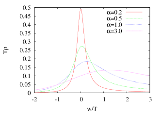
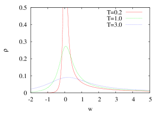
                                            a.)                                                         b.)

Figure 2: a.) The exact, normalized spectral function at $v=0$. Common features are the dominantly exponential decrease for $w\to-\infty$, power-law decrease $\sim w^{-1-\alpha/\pi}$ for $w\to\infty$ and at the peak a finite curvature $\sim\alpha$. b.) Temperature dependence of the spectral function at $v=0$. In the limit $T\to 0$ it is singular at $w=0$ point.

To discuss this result we make the following observations:

• $\bar{\varrho}(w)$ is a function of $\beta w$ only, which is understandable, since there is no other scale in the system which could form a dimensionless combination.

• For $\alpha\to 0$, we find

  $$\frac{\displaystyle e^{\beta w/2}\sin\alpha}{\displaystyle\cosh(\beta w)-\cos\alpha}\to 2\pi\delta(w),$$ (57)

  so we recover the free case. It is interesting, that this behavior periodically returns for $\alpha=2\pi n$.

• For large values of $w$ which is equivalent to the small temperature case we can use the asymptotic form of the $\Gamma$ function for complex arguments with large absolute value:

  $$\Gamma(x)=e^{-x}x^{x}\left(x^{-1/2}+{\cal O}(x^{-3/2})\right).$$ (58)

  Then we find, up to normalization factors

  $$\bar{\varrho}(\beta w\gg 1)\sim\frac{\displaystyle e^{\beta w}}{\cosh(\beta w)}\,\frac{1}{w^{1+\frac{\alpha}{\pi}}}\;\stackrel{{\scriptstyle T\to 0}}{{\longrightarrow}}\;\Theta(w)w^{-1-\frac{\alpha}{\pi}}.$$ (59)

  This is the well-known exact solution by Bloch and Nordsieck at zero temperature. Note that the $\Theta$ function came out correctly from the formula. At finite but small temperatures, for negative arguments we observe exponential decrease.

  This form also shows how at zero temperature we obtain zero wave function renormalization factor. The normalization factor (c.f. (55)) is proportional to $\beta$, while the asymptotic form is $(\beta w)^{-1-\frac{\alpha}{\pi}}$. Then approaching zero temperature we obtain $T^{\frac{\alpha}{\pi}}w^{-1-\frac{\alpha}{\pi}}$, which means a renormalization factor vanishing as $\sim T^{\frac{\alpha}{\pi}}$ for $T\to 0$.

• Now let us consider the $w\to 0$ limit, i.e. the vicinity of the mass shell. We can expand $\bar{\varrho}$ into power series

  $$\bar{\varrho}(w)=\frac{4\bar{\varrho}(0)CT^{2}}{\displaystyle(w-CT)^{2}+\left(\frac{4}{C}-1\right)C^{2}T^{2}+{\cal O}(w^{3})},$$ (60)

  where

  $$\frac{1}{C}=\frac{1}{2}+\frac{2}{1-\cos\alpha}+\frac{1}{\pi^{2}}\Psi^{2}(1+\frac{\alpha}{2\pi}),$$ (61)

  and $\Psi(a)$ is the digamma function. The maximum of this function is at $CT$, the width is $CT\sqrt{4C^{-1}-1}$. Since, however, the function is not symmetric, these parameters cannot be interpreted as a thermal mass and thermal width. For that we need to examine the real time dependence.

• For the real time dependence we use the fact that, according to (55), $\varrho(p)=\beta f_{0}(\beta(p_{0}-m))$, which means that $\varrho(t)=e^{-imt}\tilde{f}_{0}(Tt)$. Omitting the oscillating phase (i.e. if we consider the envelope of $\varrho(t)$), we recover the Fourier transform of $f_{0}$.

  The real time dependence obtained from the inverse Fourier transformation of (55) differs from (51). This is because we performed an analytic continuation to the physically sensible analytic domain. The numerical inverse Fourier transform of the normalized spectral function (and, because $iG_{ra}(t)=\Theta(t)\varrho(t)$, for $t>0$ this is also the real time dependence of the retarded Green’s function) can be seen on Fig. 3.

  

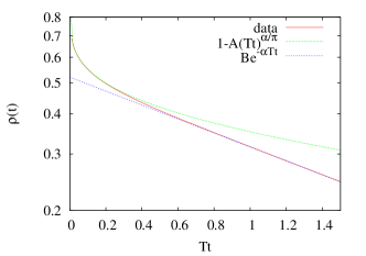
  Figure 3: Time dependence of the (envelope of the) retarded Green’s function (or, equivalently, the spectral function) for $v=0$ at $\alpha=0.5$ on a logarithmic y-scale. For small times we find $1-A(Tt)^{\alpha/\pi}$, corresponding to the zero temperature time dependence. For large times it turns into an exponential $\exp(-\alpha Tt)$ damping.

  At small times we expect to recover the zero temperature result. Indeed, we observe $\bar{\varrho}(t)=(1-A(Tt)^{\alpha/\pi})e^{-imt}$ asymptotic form (for $\alpha=0.5$ this is valid up to $Tt<0.4$), the power law time dependence is characteristic to the zero temperature result. At $t=0$ the value of the spectral function is 1, this is because of normalization. Note however, that naively at zero temperature we would obtain $\sim t^{\alpha/\pi}e^{-imt}$ time dependence, describing growth of correlation and violating the normalization condition. Interpreting the zero temperature result as $T\to 0$ limit, we could cure this apparent inconsistency of the model. At strictly $T=0$ we get back the physically sensible oscillating solution $\varrho(t)=e^{-imt}$.

  For large times (for $tT>1$) the time dependence is $\sim e^{-\alpha Tt}$, which agrees with IancuBlaizot1 ; IancuBlaizot2 . Comparing it to (51) we see that instead of an exponential rise we found an exponential decay, but with the same coefficient. This can be understood by noting that if we have a pole at $w=w_{0}$ in the momentum space, meaning $e^{-iw_{0}t}$ exponential time dependence, this pole is present in the spectral function in position $w_{0}^{*}$, too. The physical retarded Green’s function can have poles in the lower half plane, therefore we find in our case only the $w_{0}=-i\alpha T$ pole, giving exponential damping.

For the justification of the analytic continuation we also used a different method. We expanded the $t$-dependent result (51) into power series using

$$(\sinh x)^{\alpha/\pi}=\left(\frac{1}{2}\right)^{\frac{\alpha}{\pi}}\sum\limits_{k=0}^{\infty}\left[\Theta(x)(-1)^{k}{\frac{\alpha}{\pi}\choose k}e^{x(\frac{\alpha}{\pi}-k)}e^{-xk}+\Theta(-x)(-1)^{\frac{\alpha}{\pi}-k}{\frac{\alpha}{\pi}\choose k}e^{-x(\frac{\alpha}{\pi}-k)}e^{xk}\right]$$ (62)

Now the inverse Fourier transformation acts on a pure exponential function. We use the formula

$$\int\limits_{0}^{\infty}\!dt\,e^{\pm iwt-st}=\frac{1}{s\mp iw}$$ (63)

which is true, of course, if $s>0$, but this is the formula for the analytic continuation, too. Then the result of the Fourier transformation, with appropriate normalization to ensure reality of $\varrho$:

$$\varrho(w)\sim\sum\limits_{k=0}^{\infty}(-1)^{k}{\frac{\alpha}{\pi}\choose k}\left[\frac{(-1)^{-\alpha/2\pi}}{s_{k}+iw}+\frac{(-1)^{\alpha/2\pi}}{s_{k}-iw}\right],$$ (64)

where $s_{k}=\pi T(2k-\alpha/\pi)$. Using the $(-1)^{\alpha/2\pi}=\cos\frac{\alpha}{2}+i\sin\frac{\alpha}{2}$ definition we find after a simple calculation

$$\varrho(w)\sim\sum\limits_{k=0}^{\infty}(-1)^{k}{\frac{\alpha}{\pi}\choose k}\frac{s_{k}(1+\cos\alpha)-w\sin\alpha}{s_{k}^{2}+w^{2}},\qquad s_{k}=\pi T(2k-\frac{\alpha}{\pi}).$$ (65)

The sum converges fast, and we can compare the result of the two calculations on Fig. 4.

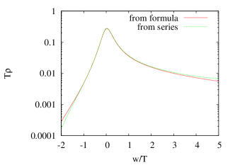
Figure 4: Comparison of the logarithm spectral function at $\alpha=0.5$ calculated from eq. (55) and from eq. (65). The two results agree well.

We can see that the two methods of analytic continuation yield consistent result in the central peak regime. To understand the small deviations at the edges, we remark that if $\alpha$ is real then $\bar{\varrho}(t=0)=0$ (c.f. (51)). In Fourier space this means $\int dw\bar{\varrho}(w)=0$, therefore it can not be positive for all momenta. Using the second method, the position where the spectral function turns into negative values is, fortunately, at large $|w/T|$ values, therefore the peak is unaffected. The only precursor of the sign changing is the slight decrease at the edges of the plot. In our first method we started from imaginary $\alpha$ values, where $\lim\limits_{t\to 0}\bar{\varrho}(t)=\bar{\varrho}_{0}\neq 0$, then the normalization does not require negative values for $\bar{\varrho}(w)$.

III.4 Finite velocity case

If $v\neq 0$ we find for eq. (47) using (36) the following formula

$$w\bar{\varrho}(w)=-\frac{\alpha}{\pi}\frac{u_{0}(1-v^{2})}{2v}\!\!\!\int\limits_{u_{0}(1-v)}^{u_{0}(1+v)}\!\!\!\frac{ds}{s^{2}}\,\int\!dq\,(1+n(\frac{q}{s}))\,\bar{\varrho}(w-q).$$ (66)

The right hand side is again a convolution, and formally we can use the same method as in the $v=0$ case. We find

$$\partial_{t}\bar{\varrho}(t)=\frac{\alpha}{\pi}\frac{u_{0}(1-v^{2})}{2v}\!\!\!\int\limits_{u_{0}(1-v)}^{u_{0}(1+v)}\!\!\!\frac{ds}{s^{2}}\,\frac{Ts}{\tanh(\pi tTs)}\bar{\varrho}(t)$$ (67)

which has the solution

$${\bar{\varrho}(t)}=\bar{\varrho}(0)\exp\left[\frac{\alpha}{\pi}\frac{u_{0}(1-v^{2})}{2v}\!\!\!\int\limits_{u_{0}(1-v)}^{u_{0}(1+v)}\!\!\!\frac{ds}{s^{2}}\,\ln(\sinh\pi tTs)\right].$$ (68)

We cannot perform analytically neither the integral, nor its Fourier transform. But we can determine many features by investigating the $t\to 0$ and $t\to\infty$ limits.

III.4.1 The limit $t\rightarrow 0$

Since $\lim\limits_{t\rightarrow 0}\sinh\pi tTs=\pi tTs$:

$$\lim_{t\rightarrow 0}\frac{u_{0}(1-v^{2})}{2v}\!\!\!\int\limits_{u_{0}(1-v)}^{u_{0}(1+v)}\!\!\!\frac{ds}{s^{2}}\,\ln(\sinh\pi tTs)=\frac{u_{0}(1-v^{2})}{2v}\!\!\!\int\limits_{u_{0}(1-v)}^{u_{0}(1+v)}\!\!\!\frac{ds}{s}\,\ln\pi tTs=\ln\pi Tt+\text{const.},$$ (69)

where the constant comes from the integral of $s^{-2}\ln s$. Being a finite quantity, it goes into the normalization. After exponentiation we find

$$\bar{\varrho}(t)\sim(Tt)^{\alpha/\pi},$$ (70)

which is the zero temperature result. So, as we expected the short time or large frequency regime reproduces the zero temperature case, and thus it is velocity-independent.

III.4.2 The limit $t\rightarrow\infty$

Here the $\sinh$ can be approximated by the exponential, and so

$$\lim\limits_{t\rightarrow\infty}\ln\sinh\pi Tts=\pi Tts-\ln 2$$ (71)

The $\ln 2$ yields a constant factor which goes into the normalization. The rest gives, including the prefactors

$$\alpha Tt\frac{u_{0}(1-v^{2})}{2v}\!\!\!\int\limits_{u_{0}(1-v)}^{u_{0}(1+v)}\!\!\!\frac{ds}{s}=\alpha_{eff}(u)Tt,$$ (72)

where

$$\alpha_{eff}(u)=\alpha\frac{u_{0}(1-v^{2})}{2v}\ln\left(\frac{1+v}{1-v}\right).$$ (73)

From this form we obtain for the spectral function in the asymptotic limit:

$$\bar{\varrho}(t)=Ce^{\alpha_{eff}(u)Tt}.$$ (74)

We can easily check that $\lim\limits_{v\to 0}\alpha_{eff}(u)=\alpha$. Therefore the $v\to 0$ limit is analytic.

Since in the asymptotic time regime we simply get the substitution rule $\alpha\to\alpha_{eff}(u)$ as compared to the $v=0$ case, the analysis of the vicinity of the peak of the spectral function, and the large time dependence will remain valid in the finite velocity case, too, with a modified value of the coupling. In particular, since $\alpha_{eff}(u)<\alpha$, we obtain a smaller damping, larger lifetime for $v>0$ cases. Physically this property is the consequence of the decreasing cross section at larger energies.

III.4.3 Solution for $t\in(0,\infty)$

For intermediate times we could not work out analytically the integral. Nevertheless, we have a well-controlled numerical method to find the spectral function, once the analytic behavior for large $t$ is identified. We express the wanted $\bar{\varrho}_{u}(t)$ as a product of the known $\bar{\varrho}_{u=0}(t;\alpha_{eff})$ and a correction factor

$$\bar{\varrho}(t)\sim Z(t)\bar{\varrho}_{u=0}(t;\alpha_{eff}),$$ (75)

where

$$Z(t)\equiv\frac{\displaystyle\exp\left[\frac{\alpha u_{0}(1-v^{2})}{2\pi v}\!\!\!\int\limits_{u_{0}(1-v)}^{u_{0}(1+v)}\!\!\!\frac{ds}{s^{2}}\ln(\sinh\pi tTs)\right]}{\displaystyle(\sinh\pi Tt)^{\frac{\alpha_{eff}(u)}{\pi}}}.$$ (76)

After a short algebra we find

$$Z(t)=\exp\left\{\frac{\alpha u_{0}(1-v^{2})}{2\pi v}\!\!\!\int\limits_{u_{0}(1-v)}^{u_{0}(1+v)}\!\!\!\frac{ds}{s^{2}}\ln\frac{\sinh\pi Tts}{(\sinh\pi Tt)^{s}}\right\}.$$ (77)

The so-defined ratio is symmetric $Z(t)=Z(-t)$. For small $t$ arguments it behaves as $Z(t)\sim(Tt)^{\frac{\alpha-\alpha_{eff}(u)}{\pi}}$ and, since $\alpha\geqq\alpha_{eff}(u)$, we also know $Z(t=0)=0$. At large $t$ we find $\lim\limits_{t\rightarrow\infty}Z(t)=1$. We can determine it numerically, for a specific $v$ it can be seen on Fig. 5

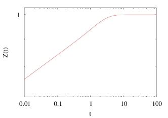
Figure 5: The $Z(t)$ function on a logarithmic plot. For small times it is a power, for larger times it flattens out.

We can numerically Fourier transform $Z(t)$, and perform a convolution in the Fourier space with the $\bar{\varrho}_{v=0}(w)$ function (51). This ensures that we use the same analytic continuation for the different velocity cases. As a result we obtain Fig. 6.

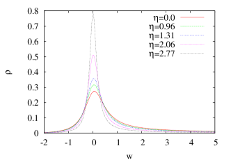
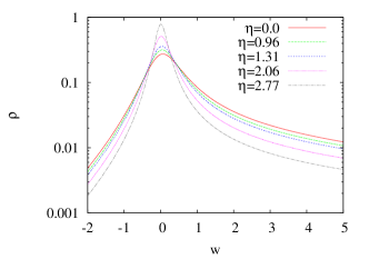
                                            a.)                                                         b.)

Figure 6: Velocity dependence of the spectral function for $\alpha=0.5$. The $\eta$ values are rapidities, $v=\tanh\eta$. a.) is a linear-linear plot to show that the peak region becomes more and more peaked with increasing $\eta$ ($v$). The log-log plot demonstrates that the asymptotics remain the same.

We can observe that the peak becomes narrower for larger velocities, corresponding to the decreasing $\alpha_{eff}$ value. At large momentum the asymptotics is the same for all velocities (for a given $\alpha$), because the zero temperature result is insensitive to the value of $v$.

Here again we can work out the real time dependence. We now write $\varrho_{u}(p)=u_{0}\beta f_{u}(\beta(p_{0}u_{0}-\mathbf{pu}-m))$ and find

$$\varrho_{u}(t)=e^{-i\mathbf{vp}t-imt/u_{0}}\tilde{f}_{u}(\frac{tT}{u_{0}}).$$ (78)

The result of the numerical inverse Fourier transform can be seen on Fig. 7.

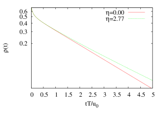
Figure 7: Comparison of the real time dependence of the retarded Green’s function (or, equivalently, the spectral function) for zero and finite velocity at $\alpha=0.5$ on logarithmic y scale. The small time behavior does not change, at large times the exponential damping turns to $\exp(-\alpha_{eff}(u)Tt)$.

At small times the spectral function (retarded Green’s function) is velocity independent, this is the zero temperature asymptotics. For large times (for $Tt>1$) the time dependence turns into $\sim e^{-\alpha_{eff}(u)Tt}$.

III.5 Discussion of earlier results

We can compare our results to the earlier results in the literature. The long time asymptotics of the finite temperature solution of the Bloch-Nordsieck model was already discussed in IancuBlaizot1 ; IancuBlaizot2 . They followed a different, functional approach. Still, the two methods lead to the same intermediate result. Neglecting renormalization effects (which is treated later in Ref. IancuBlaizot1 ; IancuBlaizot2 ), our eq. (31) together with (34) yields, using the notation $w=up-m$

$$w{\cal G}_{ra}(w)=e^{2}U^{2}{\int\!\frac{d^{4}k}{(2\pi)^{4}}\,}\frac{1}{uk}\,(1+n(k_{0}))\bar{\varrho}(k)\,\bar{\cal G}_{ra}(w-uk),$$ (79)

where $\bar{\varrho}(k)=\frac{2\pi}{2k}(\delta(k_{0}-k)-\delta(k_{0}+k))$ is the photon spectral function. After Fourier-transformation we find exponentiation of the real time contributions

$${\cal G}_{ra}(t)={\cal G}_{ra}(t=0)e^{F(t)},$$ (80)

where

$$F(t)=-e^{2}U^{2}{\int\!\frac{d^{4}k}{(2\pi)^{4}}\,}(1+n(k_{0}))\bar{\varrho}(k)\,\frac{1-e^{-iukt}}{(uk)^{2}}=-it\Phi_{0}+it\Phi(t)+\ln\Delta(t),$$ (81)

where $\Phi_{0}$, $\Phi(t)$ and $\ln\Delta(t)$ are real quantities, corresponding to the notation of IancuBlaizot2 . Using $U^{2}=1$ this means

$$\Phi(t)=-e^{2}{\int\!\frac{d^{4}k}{(2\pi)^{4}}\,}\frac{\bar{\varrho}(k)}{uk}\left[1-\frac{\sin ukt}{ukt}\right]$$

$$\Phi_{0}=-e^{2}{\int\!\frac{d^{4}k}{(2\pi)^{4}}\,}\frac{\bar{\varrho}(k)}{uk}$$

$$\Delta=\exp\left\{-e^{2}{\int\!\frac{d^{4}k}{(2\pi)^{4}}\,}n(k_{0})\bar{\varrho}(k)\,\frac{1-\cos ukt}{(uk)^{2}}\right\}.$$ (82)

These expressions agree with the equations (2.24) and (2.25) of IancuBlaizot2 (the constant phase $\Phi_{0}$ has no physical meaning).

The analysis of this formula, however, differs in our case and in IancuBlaizot1 ; IancuBlaizot2 . We strictly restrict ourselves to the original Bloch-Nordsieck model, and used the free photon spectral function. In Ref. IancuBlaizot1 ; IancuBlaizot2 the authors used HTL-improved photon spectral function (cf. their eq. (3.1) and (3.2)). As it turns out, the most important contribution comes from the small frequency limit of the continuum (Landau damping) part. This explains why the asymptotic time behavior differs in our case and in the case of Ref. IancuBlaizot1 ; IancuBlaizot2 ( $\exp(-\alpha_{eff}(v)Tt)$ vs. $\exp(-Ct\log t)$ ).

In Ref. Fried:2008tb Fried et. al. use again a different formalism. Since they examine a different physical situation, the comparison is much more difficult. What is clear, however, that they also use the original version of the model, and also find exponentially damping solution.

It is very interesting that in Wang:2000via the authors found the same $\exp(-\alpha Tt\log t)$ like solution as was the case in Ref. IancuBlaizot1 ; IancuBlaizot2 , although with a different line of thought. They use the dynamical renormalization group idea Boyanovsky:1999cy , where the secular terms are melted into finite time dependence of the renormalized parameters. Clearly they cannot consider all photonic diagrams, just those which contribute to the renormalization group (RG) equations. The logarithmic enhancement of the damping there can be interpreted physically as an eternally growing cross section of the incoming hard particle which collects more and more soft photons around itself. The analysis of the pure Bloch-Nordsieck model results in a finite damping, which means that in this model the initial growth of the cross section eventually stops, the soft photon cloud saturates. The physical interpretation of the saturation probably is that the multi-photon contributions arriving from different spacetime points become incoherent.

The two scenarios, one with ever growing photon cloud, the other with saturation, are both approximations of the real QED (RG, HTL and free photon approximations, respectively). The question that which one is finally manifested in QED, can be answered only after a full analysis of the complete QED where all these effects are present.

IV Conclusions

In this paper we studied the Bloch-Nordsieck model at finite temperature, in particular we studied the fermionic spectral function. We used the strategy introduced in Jakovac:2011aa which is based on the Dyson-Schwinger equations, where the infinite hierarchy is closed by using the Ward identities for the vertex function. We worked out the corresponding equations at finite temperature in the real time formalism, and solved them. This procedure is exact in the Bloch-Nordsieck model.

At zero velocity we were able to obtain fully analytic results for the spectral function. For large momenta and/or zero temperature this formula agrees with the zero temperature result. At finite temperature there appears an asymmetric peak which decreases exponentially below the mass shell ($u^{\mu}p_{\mu}<m$) and as a power law above the mass shell ($u^{\mu}p_{\mu}>m$).

We also worked out the real time dependence which has two characteristic regime. For small times, starting from its initial value, it behaves as a power law $\bar{\varrho}(t)=(1-A(Tt)^{\alpha/\pi})e^{-imt}$, where $A$ depends on $\alpha$. The naive zero temperature calculation yields $\sim t^{\alpha/\pi}e^{-imt}$ time dependence which is not normalizable and corresponds to a physically hardly interpretable forever growing retarded response function. With the finite temperature as a regulator, we could interpret the zero temperature result, and we got a physically sensible purely oscillating response function.

For large times we find exponential damping. The damping rate is $\alpha_{eff}(u)T$, where the effective coupling $\alpha_{eff}(u)$ is given in (73). The damping is smaller, the lifetime is longer for larger velocities, which physically can be interpreted as the consequence of decreasing cross sections. We remark that the damping in the pure Bloch-Nordsieck model differs from the one with HTL-improved photon propagator; in this latter case one finds a faster-than-exponential damping with an exponent $\sim-t\ln t$.

We expect that the method we worked out for the Bloch-Nordsieck model can be applied, as an approximation scheme, also for the full QED. Hopefully the renormalizability of the resummation will remain true, too.

- (1) F. Bloch and A. Nordsieck, Phys. Rev. 52 (1937) 54.
- (2) N.N. Bogoliubov and D.V. Shirkov, Introduction to the theories to the quantized fields (John Wiley & Sons, Inc., 1980)
- (3) H.M. Fried, Green’s Functions and Ordered Exponentials (Cambridge University Press, 2002)
- (4) H. A. Weldon, Phys. Rev. D 44, 3955 (1991).
- (5) A. I. Alekseev, V. A. Baikov and E. E. Boos, Theor. Math. Phys. 54, 253 (1983) [Teor. Mat. Fiz. 54, 388 (1983)].
- (6) A. Jakovac and P. Mati, Phys. Rev. D 85 (2012) 085006 [arXiv:1112.3476 [hep-ph]].
- (7) J. -P. Blaizot and E. Iancu, Phys. Rev. D 55 (1997) 973 [hep-ph/9607303].
- (8) J. -P. Blaizot and E. Iancu, Phys. Rev. D 56, 7877 (1997) [hep-ph/9706397], J. -P. Blaizot and E. Iancu, Phys. Rev. D 55, 973 (1997) [hep-ph/9607303].
- (9) H. A. Weldon, Phys. Rev. D 69 (2004) 045006 [hep-ph/0309322].
- (10) H. M. Fried, T. Grandou and Y. -M. Sheu, Phys. Rev. D 77 (2008) 105027 [arXiv:0804.1591 [hep-th]].
- (11) N. P. Landsman and C. G. van Weert, Phys. Rept. 145, 141 (1987); M. Le Bellac, Thermal Field Theory, (Cambridge Univ. Press, 1996.)
- (12) J. Collins, Renormalization: an introduction to renormalization, the renormalization group and the operator product expansion, (Cambridge University Press, Cambridge, 1984)
- (13) M.E. Peskin, D.V. Schroeder, An Introduction to Quantum Field Theory, (Perseus Books Publishing, 1995.)
- (14) S. -Y. Wang, D. Boyanovsky, H. J. de Vega and D. S. Lee, Phys. Rev. D 62 (2000) 105026 [hep-ph/0005223].
- (15) D. Boyanovsky, H. J. de Vega and S. -Y. Wang, Phys. Rev. D 61 (2000) 065006 [hep-ph/9909369].