Quantum-state transfer via resonant tunnelling through local field induced barriers

Abstract

Efficient quantum-state transfer is achieved in a uniformly coupled spin-$1/2$ chain, with open boundaries, by application of local magnetic fields on the second and last-but-one spins, respectively. These effective barriers induce appearance of two eigenstates, bi-localized at the edges of the chain, which allow a high quality transfer also at relatively long distances. The same mechanism may be used to send an entire e-bit (e.g., an entangled qubit pair) from one to the other end of the chain.

I Introduction

Quantum State Transfer (QST), i.e., the reliable transfer of an arbitrary quantum state between different quantum processing units, is one of the major tools of distributed quantum computing and provides the basic ‘building block’ for any quantum communication protocol Nielsen ; interkimble . When the information is encoded in intrinsically localized units, an efficient quantum communication channel can be realized with effective spin systems Bose2003 , in order to avoid the difficult problem of interfacing with flying qubits. This channel becomes especially useful for short ranged, on-chip communication (see Ref. channels and references therein).

For the QST of one qubit (which may be part of an entangled or, more generally, a correlated pair campbell ), a number of protocols have been described employing spin-$\frac{1}{2}$ chains as quantum data bus to transfer information between their first and last spins (the sender and receiver, respectively). In particular, a high Fidelity transmission can be obtained if additional resources are employed with respect to the original plain scheme of Ref. Bose2003 . Examples include the encoding of quantum states on spatially extended wave packets PaganelliGP09 ; LindenO04 , the use of local end-chain operations DiFrancoPK , of local memories and parallel quantum channels GiovannettiBB , or of protocols employing time-dependent interactions timedependent . A perfect state transfer, which is unattainable in a uniformly coupled chain, can be achieved instead by a proper pre-engineering of the coupling strengths. The key advantage in this case is that no external time dependent controls are needed, as the transfer is realized through the intrinsic dynamics of the chain. Perfect QST, which may be thought of as a particular instance of a more generic swap operation swap , is entailed by accurate settings of the intra-channel coupling strengths giving rise to a linear dispersion relation for excitations propagating across the channel Christandl2004 . However, dispersion during transmission occurs in most spin chains due to the nontrivial structure of the many-body Hamiltonian describing the channel, and the design of a non-dispersive channel requires a demanding engineering of the Hamiltonian parameters. A systematic analysis on how to set the couplings to allow for a perfect state transfer can be found in Refs. vinet85 ; bruderer .

On the other hand, a quasi perfect transfer vinet can be obtained by modifying only a few couplings of an otherwise homogeneous quantum channel CamposVenutiET08 , in order to obtain a ballistic excitation transfer BACVV , or Rabi-like oscillations between eigenstates having support only on the sender and receiver sites Wojcik2005 ; Gualdi08 ; Plastina2007 ; PaganelliPG2006 ; heule ; linne .

In this work, we propose a new transfer protocol of the latter kind and analyze the efficiency and reliability of state transmission in presence of a minimal engineering, which depends on the resonant tunnelling of spin excitations induced by application of local magnetic fields near the sending and receiving sites. Specifically, we require the sender and receiver to have access and control over the local fields applied on their neighboring spins, which are increased by $\omega$ with respect to the rest of the chain (see the sketch in Fig. 1). As discussed in Ref. Plastina2007 ; PaganelliPG2006 ; apo06 , in an open spin-$1/2$ chain of $N$ nodes, these extra local fields induce appearance of two single-particle states, which are ‘bi-localized’ on sites $2$ and $N-1$ and can be exploited to perform QST between them heule ; linne in a time $t{\sim}\omega^{N-2}$. However, this is not the only effect produced by the local fields. The geometric confinement, due to the open boundary conditions imposed on the chain, induce appearance of a further pair of eigenstates which are localized on the first and last sites and can be exploited for a much faster QST. Indeed, once the spin chain is fermionized via the Jordan-Wigner transformation, it is easy to recognize that the local fields create effective potential barriers for the single-particle excitations. If these barriers have equal heights (thus establishing a mirror symmetry shi ), a coherent resonant tunnelling occurs between the first and last sites, giving rise to information transfer.

The paper is organized as follows: in Sec II the model with the magnetic field ‘barriers’ is solved, and the appearance of the bi-localized states mentioned above is discussed; in Sec. III the transmission Fidelity is studied and the effectiveness of the local fields allowing for a very high quality QST is demonstrated. Furthermore, in subsection III.2 the resilience with respect to noise is analyzed, while in subsection III.3 the possibility of transferring more than one qubit is briefly touched upon. After that, in Sec. IV, a time-dependent protocol based on the switching of the local fields is presented and, finally, some concluding remarks are drawn in Sec. V.

II The model and its properties

We consider a linear chain of spin-${1}/{2}$ particles residing at sites, $n{=}1,2,...,N$, in a lattice of unit lattice constant. The $N$ spins are coupled through the homogeneous nearest-neighbor $XX$ model

$$\mathcal{H}=-J\left\{\dfrac{1}{2}\sum_{n{=}1}^{N{-}1}(\sigma_{n}^{x}\sigma_{n{+}1}^{x}{+}\sigma_{n}^{y}\sigma_{n{+}1}^{y})+\sum_{n=1}^{N}K_{n}\sigma_{n}^{z}\right\},$$ (1)

here expressed in $\hbar{=}1$-units, which will be used throughout this paper. In Eq. (1), $\sigma_{n}^{\alpha}$ ($\alpha{=}x,y,z$) are the usual Pauli matrices for the spin at the $n$-th site, probed by a local magnetic field of intensity $K_{n}$, and $J$ is the exchange coupling strength between two nearest neighboring sites. In the following $J$ will be set to $1$ and taken as our energy unit (therefore, times will be given in $1/J$ units).

As in the protocol of Ref. Bose2003 , we begin with the chain being prepared with all spins up, say, in the initial state $\left|\textbf{0}\right\rangle{=}\left|0\right\rangle^{\otimes N}$ in which $\left|0\right\rangle$ and $\left|1\right\rangle$ denote the spin-up and down states along the $z$ axis, respectively. Next, we initialize the first spin of the chain to the state $\left|\psi_{in}\right\rangle{=}\alpha\left|0\right\rangle+\beta\left|1\right\rangle$ and let the chain follow the time-evolution generated by the Hamiltonian (1). Since $[\mathcal{H},\sum_{n=1}^{N}\sigma_{z}^{n}]{=}0$, the dynamics take place in the invariant subspaces with $0$ and $1$ flipped spins, where the former is made up of the state $\left|\textbf{0}\right\rangle$ alone, while the latter is spanned by the computational basis states $|\textbf{j}\rangle=\sigma_{j}^{+}|\textbf{0}\rangle\equiv|0_{1},0_{2},\ldots,0_{j-1},1_{j},0_{j+1},\dots\rangle$.

The state of the last spin, $\rho_{N}(t)$, is obtained from the time evolved state of the chain by tracing out all but the $N$-th spin, and the aim of the QST protocol is to retrieve the state encoded in the first spin from the last one. The efficiency of the state transfer is then quantified by the Fidelity $F(t){=}\left\langle\psi_{in}\right|\rho_{N}(t)\left|\psi_{in}\right\rangle$, which equals $1$ in the case of a perfect transfer. In order to evaluate the channel quality independently of the specific input state, we refer to the average Fidelity ${\overline{F}}(t)$ by integrating $F(t)$ over all possible pure input states of a qubit. This leads to

$${\overline{F}}(t)=\frac{|f_{N1}(t)|}{3}+\frac{|f_{N1}(t)|^{2}}{6}+\frac{1}{2},$$ (2)

where $f_{N1}(t)=\langle\textbf{N}|e^{-i{\cal{H}}t}|\textbf{1}\rangle$ is the transition amplitude of a spin excitation from the first to the last site of the chain. In the following, with the term Fidelity we will refer to the quantity given by Eq. (2).

The same effective channel can be used to transfer entanglement, with the first spin sharing an initial singlet state with an external and uncoupled qubit. The amount of (transferred) entanglement between the last spin of the chain and the external one at a subsequent time $t$, as measured by the Concurrence, is given by Bose2003

$$C(t)=|f_{N1}(t)|.$$ (3)

Therefore, in order to perform efficiently both of the tasks, namely the state and entanglement transfers, it is necessary to achieve a value of $|f_{N1}(t)|$ as close as possible to $1$ at a certain time $t^{*}$.

Because of the time invariance of the subspaces with a given number of flipped spins, the calculation of $f_{N1}(t)$ is reduced to diagonalizing the Hamiltonian in the single excitation sector, where Eq. (1) can be expressed as a tri-diagonal matrix whose elements are $\mathcal{H}^{(1)}_{nm}{=}2K_{n}\delta_{nm}{-}\left(\delta_{n,n+1}+\delta_{n,n-1}\right)$. Indeed, the transition amplitude $f_{N1}$ can be written as

$$f_{N1}(t){=}\sum_{k=1}^{N}\langle\mathbf{N}|\mathbf{a}_{k}\rangle\langle\mathbf{a}_{k}|\mathbf{1}\rangle e^{-i\lambda_{k}t}$$ (4)

where $\lambda_{k}$ are the eigenvalues and $|\mathbf{a}_{k}\rangle{=}\sum_{j=1}^{N}a_{kj}|\mathbf{j}\rangle$ the corresponding eigenvectors of $\mathcal{H}^{(1)}$, arranged in increasing order, i.e., $\lambda_{k^{\prime}}{>}\lambda_{k}$ for $k^{\prime}{>}k$.

As we will show below, a large value for $|f_{N1}|$ can be obtained by modifying only two local fields in such a way that only two eigenvectors among the $|\mathbf{a}_{k}\rangle$’s have a non-negligible superposition with $\left|\mathbf{1}\right\rangle$ and $\left|\mathbf{N}\right\rangle$. Correspondingly, the time evolution induced by ${\cal H}$ gives rise to an effective Rabi oscillation of the spin-excitation between the first and the last sites of the chain.

Specifically, we assume that the local magnetic fields are applied to the second and last-but-one spins, which in the following will be denoted as barrier qubits, by setting $K_{n}{=}\omega\left(\delta_{n,2}+\delta_{n,N-1}\right)$ in Eq. (1), which gives rise to the model depicted in Fig. 1. This yields an effective decoupling of the first and the last spins of the chain whose dynamics take place mainly in a subspace spanned by two particular eigenstates of $\mathcal{H}^{(1)}$, which are close enough in energy and bi-localized at the edges of the chain.

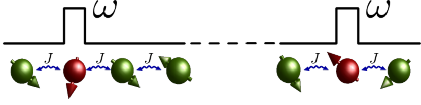
Figure 1: (color on-line): Sketch of the spin chain with sender and receiver located at the first and last sites, and with local field barriers of height $\omega$ applied to the second and last-but-one sites.

To confirm these expectations, we study the spectrum of ${\cal{H}}^{(1)}$, reported in Fig. 2 for spin chains of $N{=}17,18$ sites. The cases of even and odd site numbers are analyzed separately, as they display slightly different features.

In order to quantify the localization of the eigenvectors $\left|\mathbf{a}_{k}\right\rangle$, induced by the magnetic field $\omega$, we use the Inverse Participation Ratio (IPR), whose application to state transfer has been discussed in Ref. ZwickO2011 , which is defined as

$$\mbox{IPR}(\left|\mathbf{a}_{k}\right\rangle){=}\dfrac{\sum_{i=1}^{N}|a_{ki}|^{2}}{\sum_{i=1}^{N}|a_{ki}|^{4}}.$$

When a state is localized on a single site $n$, i.e., $a_{ki}{=}\delta_{ni}$, the IPR takes its minimum possible value $\mbox{IPR}=1$. On the other hand, an extended state distributed over a large number of sites yields an IPR value of the order of the chain length. Notice that the IPR gives information about the degree of localization of a given eigenstate only, but it does not say anything about its spatial distribution (with the exception of the $\mbox{IPR}{=}N$ case, corresponding to a state uniformly spread over the whole system).

In Fig. 3, we report the IPR of the eigenstates, ordered by ascending eigenvalues, for $N=17$ and $18$. The effect of increasing $\omega$ is twofold. First, it causes a strong localization of the two eigenvectors $\left|\mathbf{a}_{1,2}\right\rangle$: IPR$(\left|\mathbf{a}_{1,2}\right\rangle){\simeq}2$. These are the two lowest-lying eigenvalues, emerging out the unperturbed ($\omega{=}0$) energy band $\lambda_{k}{\in}(-2,2)$ (see Fig. 2). By increasing $\omega$, these states localize on the two barrier qubits and therefore their contribution to the quantity in Eq. (4) is negligible. Second, another pair of eigenvectors is found, with positive energies close to zero, which reduce their IPR to a value asymptotically tending to $2$ for even site numbers (Fig. 3b), while remaining slightly above $2$ for odd site numbers (Fig. 3a).

The localization properties of these eigenstates are crucial for quantum-information transfer as they turn out to give the main contributions in Eq. (4). The remaining intra-band eigenstates hold their extended nature and, for even $N$, they have a negligible superposition with the states $\left\{\left|\mathbf{1}\right\rangle,\left|\mathbf{N}\right\rangle\right\}$, so that the dynamics occur in an effective two-level subspace. On the other hand, in the odd-$N$ case, an eigenvector with zero energy eigenvalue is present, which, independently of $\omega$, has a constant amplitude on the sender and receiver sites, given by $\sqrt{\frac{2}{N+1}}$ . As a consequence, its contribution to Eq. (4) cannot be neglected for short chains, and the resulting effective dynamics involve three levels.

Figure 2: (color online): Spectrum of a spin chain with $N{=}17$ (upper panel) and $N{=}18$ sites (lower panel) versus $\omega$: in both cases, the two lowest eigenenergies move outside the band as $\omega$ increases, while the two positive eigenenergies closest to zero become quasi-degenerate. The latter are represented by red, solid lines. A zero-energy eigenstate occurs in the odd chain, whose eigenvalue is represented by the green dot-dashed line. All energies values are reported in units of $J$.

Furthermore, from Fig. 2 we see that other intra-band eigenvalues experience a downward shift and the eigenvalues of the bi-localized states become quasi-degenerate with energies close to zero.

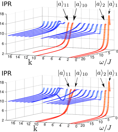
Figure 3: (color online): $\mathsf{IPR}$ for the eigenstates $\left|a\right\rangle_{k}$ of a chain of $N{=}17$ (upper plot) and $N{=}18$ (lower plot) sites, sorted by increasing eigenvalues, versus $\omega$ (in units of $J$). The first two eigenstates, $\left|a\right\rangle_{1}$ and $\left|a\right\rangle_{2}$, rapidly reach $IPR{\simeq}2$, becoming bi-localized on the barrier qubits . The states corresponding to $k=10,11$, which bi-localize on the sender and receiver qubits, reach the value $\mbox{IPR}{\simeq}2$ for the even chain, whereas one of them remains slightly above that value for the odd chain.

With these results at hand, we are now in position to evaluate the transition amplitude $f_{N1}$, and then the Fidelity (2) and the Concurrence (3).

III Figures of merit for the transmission

The average transmission Fidelity and the transmitted Concurrence are reported in Fig. 4, both as functions of time and chain length, for fixed values of the auxiliary local fields $\omega$ applied to the second and last-but-one sites. To better appreciate the results, they are compared with the homogeneous case $\omega{=}0$. In Fig. 4 a we observe a significant improvement of Fidelity and Concurrence in presence of $\omega$ with respect to the homogeneous case, while Fig. 4 b shows that the difference becomes more and more pronounced with increasing the chain length. Indeed, at $\omega{=}0$, many terms enter the sum (4), giving rise to a destructive interference that rapidly suppresses the transfer efficiency (as measured both by Fidelity and Concurrence). On the other hand, in presence of the auxiliary fields $\omega$, only two eigenvectors enter significantly the transition amplitude $f_{N1}(t)$ so that both the state and entanglement transfers are of high quality.

(a)                                   (b)

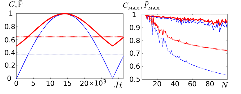
Figure 4: (color online): a) Fidelity (red thick line) and Concurrence (blue thin line, starting from $C=0$ at $t=0$) for a chain of $N=100$ spins with $\omega{=}100J$. The dashed red and blue lines are, respectively, the maximum value of the Fidelity and of the Concurrence attainable for the homogeneous chain with $\omega{=}0$. Time is expressed in units of $J^{-1}$. b) Maximum of Fidelity (red thick line) and Concurrence (blue thin line) versus the number of sites $N$ for $\omega{=}10J$ (solid line) and $\omega{=}0$ (dashed line)

In Fig. 5 we report the density plot of the maximum Fidelity as a function of the number of sites and intensity $\omega$ of the local fields to show that even modest values of $\omega$ are sufficient for high-fidelity state transfer.

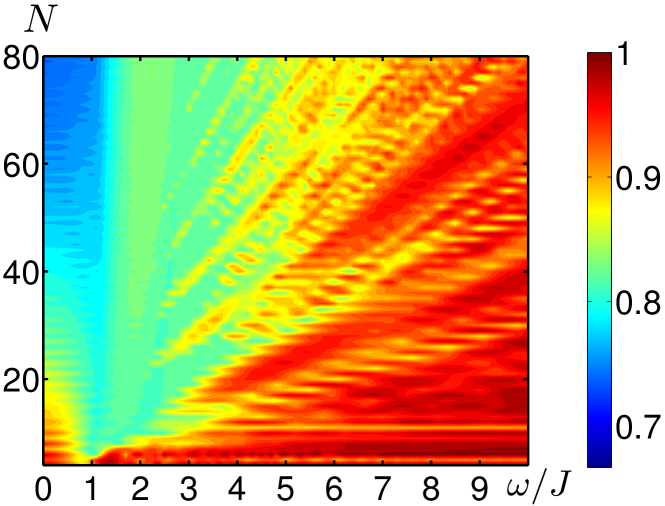
Figure 5: (color online): Maximum Fidelity in the time interval $Jt{\in}\left[0,4000\right]$ as function of $\omega$ (in units of $J$) and $N$. Notice that for $\omega{=}0$ the Fidelity is larger than $0.9$ only for short chains, while, as $\omega$ increases, the Fidelity is significantly enhanced.

By increasing $\omega$, the localization effect is enhanced and, as a result, a better quantum-state transfer is obtained. This is demonstrated in Fig. 6, where the attainable Fidelity tends towards $1$ both for even and for odd site numbers. Nevertheless, as the eigenvalues of the bi-localized eigenvectors become closer and closer to each other, by increasing $\omega$, the transfer time increases. Since the transfer is based on Rabi-like oscillations between the two eigenvectors with IPR${\simeq}2$, the transfer time $t_{\mathsf{MAX}}$ can be obtained from their eigenvalues: $t_{\mathsf{MAX}}{=}\pi/(\lambda_{2}-\lambda_{1})$, where $\lambda_{2}{>}\lambda_{1}$. Furthermore, as shown by a straightforward perturbation analysis, the eigenvalue difference scales as $(N\omega)^{-1}$ for odd site numbers, while it behaves as $\omega^{-2}$ for even ones, resulting in shorter transfer times for odd $N$ (see Fig. 6b). Notice that the optimal transfer time does not directly depend on $N$ for even site numbers, but $\omega$ needs to be increased (almost linearly) with increasing $N$ in order to have a Fidelity that stays close to unity.

(a)                                   (b)

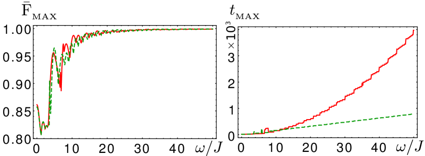
Figure 6: (color online): a) Maximum Fidelity achievable in the time interval $Jt{\in}\left[0,4000\right]$. b) Optimal times at which the best transmission is attained. The plots refer to chains of $N=22$ (red solid line) and $N=23$ sites (green dashed line). For odd (even) $N$, $t_{\mathsf{MAX}}$ is linear (quadratic) in $\omega$.

III.1 Effective Hamiltonian description

In this section, we compare our results with those obtained using weak-end bonds Wojcik2005 . To this end, we consider a uniform magnetic field applied to a chain with sender and receiver sites coupled more weakly to their neighboring spins than the other nearest neighboring sites. Such a week bond is characterized by an interaction strength $J^{\prime}$, being smaller than the intra-chain exchange $J$. It turns out that a large Fidelity can be obtained provided the ratio $J^{\prime}/J$ is suitably reduced with increasing the chain’s length. Moreover, with weak end-bonds, a similar behavior of the transfer time is obtained, with an even/odd asymmetry akin to the one discussed above.

The similarity is explained by observing that the magnetic field barriers on the second and last-but-one spins give rise to effective weak-end bonds, which, however, display some differences with respect to the set-up of Ref. Wojcik2005 . From a perturbation analysis in terms of the small parameter $J/\omega{\ll}1$, we infer that the main effect of the local fields is to modify the exchange interaction strengths between pairs of spins near the sender and receiver sites. Indeed, the effective Hamiltonian for the first three spins of the chain reads

$$H_{\mbox{eff}}{=}-\left(\lambda_{+}\left|\psi_{+}\right\rangle\left\langle\bf 3\right|-\lambda_{-}\left|\psi_{-}\right\rangle\left\langle\bf 3\right|+\mbox{h.c.}\right).$$ (5)

where, up to normalization factors, $\left|\psi_{+}\right\rangle{\propto}\lambda_{-}\left|\bf 1\right\rangle{+}\left|\bf 2\right\rangle$, $\left|\psi_{-}\right\rangle{\propto}\lambda_{+}\left|\bf 1\right\rangle{+}\left|\bf 2\right\rangle$, and $\lambda_{\pm}{=}(\omega{\pm}\sqrt{\omega^{2}+1})$. In the $\omega/J{\to}\infty$-limit, we get $\left|\psi_{+}\right\rangle{\rightarrow}\left|\bf 2\right\rangle$ and $\left|\psi_{-}\right\rangle{\rightarrow}\left|\bf 1\right\rangle$, so that the leading effect of the local fields is the appearance of effective couplings $J_{13}$ and $J_{23}$ between the corresponding spins. The latter are given by

$$J_{13}\simeq-\frac{1}{2\omega}\qquad J_{23}\simeq-\frac{1}{2}\left(1{-}\frac{1}{\omega^{2}}\right).$$

Summarizing, the effective hamiltonian of the first three spins of the chain becomes $H_{\mbox{eff}}{=}J_{13}\left(\sigma^{x}_{1}\sigma^{x}_{3}{+}\sigma^{y}_{1}\sigma^{y}_{3}\right)+J_{23}\left(\sigma^{x}_{2}\sigma^{x}_{3}{+}\sigma^{y}_{2}\sigma^{y}_{3}\right){+}\lambda_{-}\sigma^{z}_{1}{+}\lambda_{+}\sigma^{z}_{2}$; moreover, due to the presence of the large magnetic field on spin 2, its dynamics is frozen in the $\left|0\right\rangle$ state. Similar results hold for the spins near the receiver.

Once the spins at sites $2$, $N-1$ are adiabatically eliminated, we are effectively left with a chain of $N{-}2$ spins in a zero magnetic field, uniformly coupled but for the end-bonds, where the (effective) couplings between the spins $(1,3)$ and $(N-2,N)$ have strength $J_{13}$.

A further perturbative analysis in the $J_{13}{\ll}1$ limit, performed along the lines of Ref. Wojcik2005 , allow us to write an overall effective hamiltonian involving the spin-up states at the sending and receiving sites only. More precisely, this is strictly true only if $N$ is even; for a chain with an odd number of sites, instead, the inclusion of an auxiliary state is necessary, corresponding to the zero-energy eigenstate, whose effects have been discussed in Section II.

As a result, for $N$ even and odd, respectively, the state transfer is described by the following effective Hamiltonians:

$$H_{\mbox{eff}}^{even}{=} -\!\left(\frac{1}{4\omega^{2}}\left|\mathbf{1}\right\rangle\!\left\langle\mathbf{N}\right|+\mbox{h.c.}\right)$$ (6)

$$H_{\mbox{eff}}^{odd}{=} \frac{1}{2\omega}(1-\frac{4}{N-3})(\left|\mathbf{1}\right\rangle\!\left\langle\mathbf{1}\right|+\left|\mathbf{N}\right\rangle\!\left\langle\mathbf{N}\right|){+}$$ (7)

$$-\sqrt{\frac{2}{N-3}}\omega\left(\left|\mathbf{1}\right\rangle\!\left\langle a\right|_{\frac{N{+}1}{2}}+\left|\mathbf{N}\right\rangle\!\left\langle a\right|_{\frac{N{+}1}{2}}+\mbox{h.c.}\right)$$

III.2 Robustness against Noise

In this subsection we investigate how a static disorder in the magnetic fields acting on the qubits $n{=}3,..,N{-}2$ affects the efficiency of information transfer, and in particular, to be specific, of Entanglement transfer, performed according to the scheme depicted in Fig. 7. In this setting the Entanglement, initially contained in the state $\left|\Psi_{+}\right\rangle{=}\frac{1}{\sqrt{2}}(\left|01\right\rangle{+}\left|10\right\rangle)$ of the qubit pair $(0,1)$, is transferred to the pair $(0,N)$ and is quantified by the Concurrence as given by Eq. (3).

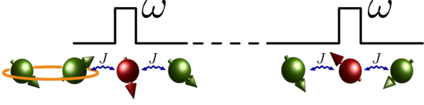
Figure 7: (color online): Scheme of the set-up used for entanglement transfer from the qubit pair $(0,1)$ to the pair $(0,N)$, where the qubit $0$ is decoupled from the chain.

The kind of disorder we consider is given by the presence of random local magnetic fields between the barrier qubits. In other words, we are assuming that local random magnetic fields, uniformly distributed in an interval $-b<K_{n}<b$, with $b$ denoting the disorder strength, act on the spins residing on sites $n=3,\ldots,N{-}2$. This choice is justified by the fact that the hamiltonian parameter of the qubits $(1,N)$ are generally considered to be more precisely controllable in order to perform efficiently the state encoding and read-out procedure and, therefore, they will be practically unaffected by the disorder. Furthermore, we allow the same degree of control for the neighboring spins $2,N-1$, whose local fields are assumed to be precisely fixed. In Figs. 8, we see that the attainable Concurrence (3), averaged over $10^{5}$ samples of disorder, remains quite high provided that $b{\ll}\omega$. Indeed, the bi-localized nature of the relevant eigenstates is not significantly perturbed. On the contrary, this is not anymore the case for values of $b$ comparable to- or greater than- $\omega$. Similar results are obtained for the Fidelity of the QST.

Depending on the specific physical implementation of the model, other sources of errors (and, specifically, of static disorder) can be identified. In particular, we would like to mention that the robustness of different transfer schemes against bond disorder, (that is, static disorder in the spin-coupling strengths) has been investigated in Ref. ZwickASO2011 . It turns out that the localization properties of the eigenstates play an important role for efficient state transfer in presence of non-uniform bonds, and that a mechanism based on localized states, like the one we are describing, is more resilient then a ballistic transport-based one.

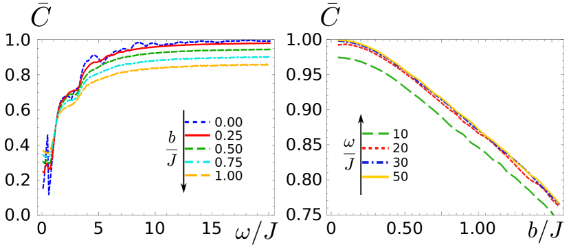
Figure 8: (color online): (left panel) Averaged Concurrence vs auxiliary field strength $\omega$ for different values of the disorder parameter $b$. (rigth panel) Concurrence vs disorder strength $b$ for different values of $\omega$. The curves for $\omega{>}20$ are almost indistinguishable and no relevant change in the effects of the disorder is observed. In both panels, the length of the chain is $N{=}10$ and averages are performed over $10^{5}$ realizations of disorder. All energy values are expressed in units of $J$.

On the other hand, since we consider high magnetic field applied locally to sites $2$ and $N-1$, a leakage effect is certainly possible, affecting the neighboring sites. To check the robustness of our transfer scheme against this lack of control, we can consider random magnetic fields, with amplitude decaying with the distance, to affect the dynamics of spins $3,4,N-3,N-2$ (on the other hand, as discussed above, we assume a very high degree of control on the sending and receiving sites, and on the barrier fields). The results of such an analysis are reported in Fig. 9, where the transmission fidelity averaged over $10^{5}$ realization of these static random fields is displayed. For very small values of the local fields $\omega$, the quality of the transfer is strongly reduced by the presence of this kind of disorder, while its effect is shown to substantially decrease for larger values of barrier fields, despite the residual static random fields are bounded always by the same fractions of $\omega$.

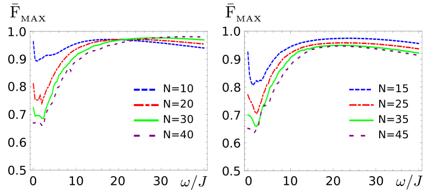
Figure 9: (color online): Averaged Fidelity vs auxiliary field strength $\omega$ for different lengths of the chain. In this case a residual magnetic field is supposed to act on sites $3,N-2$ and $4,N-3$, with random values uniformly distributed between $0$ and $\omega/10$ for the sites near the barriers, and between $0$ and  $\omega/40$ the the next to nearest sites, respectively. The plots show averages performed over $10^{5}$ realizations.

The plots suggest that, both for chains with odd and even $N$, an optimal value of the local barrier fields exists in the case in which a given fraction of it is assumed to leak to the neighboring sites. If such an optimal value of $\omega$ is selected (which scales almost linearly with the size $N$), the average fidelity is kept very close to unity.

III.3 Transport of an entire e-bit

We have shown above that a qubit encoded on the first spin of the chain is almost perfectly transferred to the other end, thanks to the application of local magnetic fields to the adjacent spins to the sender and the receiver sites. In this subsection we extend this idea to the transfer of an entangled pair. Considering the setup depicted in Fig. 10, we aim at transferring the Entanglement shared by qubits $1$ and $2$ to qubits $N{-}1$ and $N$ by use of auxiliary magnetic fields applied to sites $3$ and $N{-}3$. We, thus, allow $K_{n}{=}\omega\left(\delta_{n,3}+\delta_{n,N-2}\right)$ in Eq. (1).

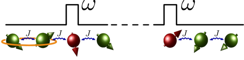
Figure 10: (color online): Sketch of the configuration for the transfer of an e-bit.

Then, we start from the fully polarized state $\left|{\mathbf{0}}\right\rangle$, and initialize the first two spins in a state belonging to the single excitation subspace so that the initial state of the whole chain reads:

$$|\Psi(0)\rangle=\alpha|\textbf{1}\rangle+\beta|\textbf{2}\rangle\;\;\;\;\;\;(\left|\alpha\right|^{2}+\left|\beta\right|^{2})=1,$$ (8)

whose evolution is given by

$$\left|\Psi(t)\right\rangle{=}\sum_{j=1}^{N}p_{j}|\mathbf{j}\rangle,\quad p_{j}=\alpha\left\langle\textbf{j}\right|e^{-iHt}\left|\textbf{1}\right\rangle{+}\beta\left\langle\textbf{j}\right|e^{-iHt}\left|\textbf{2}\right\rangle.$$ (9)

Finally, we obtain the state of the qubits $N{-}1$ and $N$ by performing the partial trace over the first $N{-}2$ spins. Considering an initially entangled $(1,2)$ pair (that is, $\alpha,\beta{\neq}0$), the amount of entanglement transferred to the pair $(N-1,N)$ and measured by the Concurrence is given by $C_{N-1,N}{=}2|p_{N-1}p_{N}|$. As shown in Fig. 11 where an initial maximally entangled state has been taken, i.e., $\alpha{=}\beta{=}\frac{1}{\sqrt{2}}$, also the Entanglement may be efficiently transferred in the presence of the auxiliary magnetic fields.

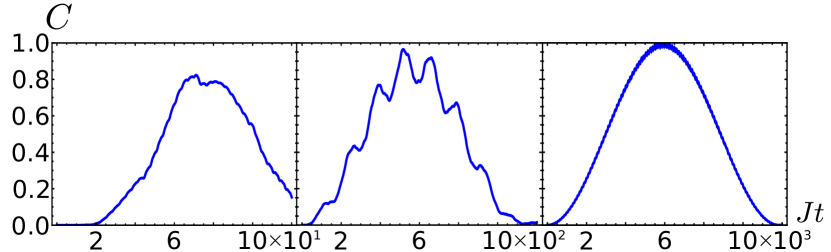
Figure 11: (color online): Concurrence transferred from the maximally initial entangled qubits pair $(1,2)$ to the pair $(N{-}1,N)$ for a chain of $N{=}33$ and $\omega{=}5,15,45$ (from left to right). Higher values of the local field, beside increasing the amount of transferred Entanglement, regularize the dynamics.

IV Time-dependent Quantum State Transfer Protocol

In this Section we investigate a QST protocol in which we allow for time-control of the magnetic fields acting on the barrier qubits. The aim of this control is to provide a precise timing for the beginning and end of the sending stage, as given by the switching of the local fields. At the same time, the control relaxes the need of a fast (in fact, instantaneous) extraction of the received information at the site $N$ once the transmission is performed. The idea is to encode the quantum state on the sender site and leave it there for a future transmission by means of a strong magnetic field on its neighbor barrier qubits. In this first step the information stays localized on the sender as no tunnelling of the spin excitation is possible due to the energy mismatch with other sites. The sending stage is then realized by switching on the magnetic field of the other barrier, at the $(N-1)$-th site. During this second step, the Rabi oscillation described in the previous Sections takes place. Finally, in the third stage, only the barrier on the last-but-one spin is left on, in order to trap the received quantum state, while the local field near the sender site is switched off.

To implement this proposal, we exploit the time-dependent Hamiltonian

$$\mathcal{H}(t)=-\dfrac{1}{2}\sum_{n=1}^{N-1}(\sigma_{n}^{x}\sigma_{n+1}^{x}{+}\sigma_{n}^{y}\sigma_{n+1}^{y}){-}\sum_{i=2,N{-1}}\omega_{i}(t)\sigma_{i}^{z},$$ (10)

where

$$\begin{array}[]{ccc}\omega_{2}(t){=}\begin{cases}K_{1}&\\ K_{2}&\\ 0&\\ \end{cases}\end{array}\quad\begin{array}[]{ccc}\omega_{N-1}(t){=}\begin{cases}0&t_{0}{\leq}t{<}t_{1}\\ K_{2}&t_{1}{\leq}t{\leq}t_{2}\\ K_{1}&t{>}t_{2}\end{cases}\end{array}$$ (11)

Here, $t_{2}{=}t_{1}{+}\Delta t$, with $\Delta t$ being an optimal transfer time interval, that we define below.

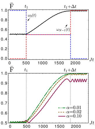
Figure 12: (color online): (upper panel) Average Fidelity for a chain of $N{=}30$ sites with $K_{1}{=}60$ and $K_{2}{=}30$, where the three steps of the QST-protocol are clearly visible from the time behavior of the two fields, which are switched according to the recipe of Eq. (11). (lower panel) Same as in the upper plot, but with finite switching times for the fields. In this case, $\omega_{2}(t)$ and $\omega_{N-1}(t)$ are smother versions of the step functions of Eq. (11), with exponential corrections: $\omega_{2}(t)=K_{2}/(\exp\{\alpha(t-t_{2})\}+1)+(K_{1}-K_{2})/(\exp\{\alpha(t-t_{1})\}+1)$, and a similar behavior for $\omega_{N-1}(t)$. The three curves correspond to three values of $\alpha$ and it turns out that the achievable ${\overline{F}}$ decreases with the steps becoming smoother and smoother (that is, with increasing $\alpha$).

With this time-dependent field configuration, the spin at the first site is “frozen” until $t{<}t_{1}$ as the state $\left|\mathbf{1}\right\rangle$ is an approximate eigenstate of $\mathcal{H}(t{<}t_{1})$; then, after the resonant tunnelling to the receiving site $t_{1}{\leq}t{\leq}t_{1}{+}\Delta t$, for $t{>}t_{2}$, the information is definitely stored in the $N$-th spin, as $\left|\mathbf{N}\right\rangle$ is an approximate eigenstate of $\mathcal{H}(t{>}t_{2})$ [see the upper panel in Fig.12].

Since the transition amplitude is given by $\left\langle N\right|U(t)\left|1\right\rangle$, in order to obtain the Fidelity, one needs to solve the time dependent Schrödinger equation for the state $U(t)\left|1\right\rangle{=}\sum_{k{=}1}^{N}\beta_{k}(t)\left|k\right\rangle$ that reduces to an $N{\times}N$ system of differential equations:

$$\begin{cases}i\dfrac{d\beta_{1}(t)}{dt}{=}-\beta_{2}(t)\\ i\dfrac{d\beta_{2}(t)}{dt}{=}-\beta_{1}(t)-\omega_{2}(t)\beta_{2}(t)-\beta_{3}(t)\\ ...\\ i\dfrac{d\beta_{j}(t)}{dt}{=}-\beta_{j-1}(t)-\beta_{j+1}(t)\;\;\;\;(j=3,...,N-2)\\ ...\\ i\dfrac{d\beta_{N-1}(t)}{dt}{=}-\beta_{N-2}(t)-\omega_{N-1}(t)\beta_{N-1}(t)-\beta_{N}(t)\\ i\dfrac{d\beta_{N}(t)}{dt}{=}-\beta_{N-1}(t).\\ \end{cases}$$ (12)

The solution, in each time interval where $\omega_{2}(t)$ and $\omega_{N-1}(t)$ are constant, is

$$\beta_{s}(t_{i+1}){=}(-1)^{s+1}\sum_{\lambda_{j}}\sum_{k=1}^{N}\frac{Q_{k,s}(\lambda)}{\frac{dP(\lambda)}{d\lambda}}|_{\lambda_{j}}e^{-i\lambda_{j}t}\beta_{k}(t_{i}).$$ (13)

where $\lambda_{j}$ are the eigenvalues of $H(t_{i})$, while $P(\lambda)$ and $Q_{k,j}(\lambda)$ are, respectively, the determinant and the minors of the matrix $(H(t_{i+1})-\lambda 1\!\!1)$. In order to perform the state transfer along the chain, the optimal time $\Delta t$ is proportional, again, to the inverse of the eigenvalues difference of the intermediate stage Hamiltonian, and reads

$$\Delta t{=}\begin{cases}\dfrac{\pi}{2}K_{2}^{2}\qquad\qquad\qquad N\;\;even\\ \\ \dfrac{\pi}{4}(N-3)K_{2}\qquad\;\;N\;\;odd.\end{cases}$$

The procedure works quite well for even $N$, as illustrated in Fig. 12, where the detrimental effect of finite switching times for the field is also explored. Unlike adiabatic transfer schemes Chenetal12 , here a fast switching of the magnetic fields is desirable because the overlap of the initial (final) state $\left|\mathbf{1}\right\rangle$ ($\left|\mathbf{N}\right\rangle$) with the bi-localized states is maximized by a step function, whereas a smoother switching function would introduce into the dynamics destructively interfering states that do not possess the required localization properties. This is illustrated in the lower panel of Fig.12, where the average Fidelity is plotted for different switching rates.

For odd chains, on the other hand, the presence of the zero-energy eigenstate taking part in the dynamics, makes the state transfer more involved, because the trapping stages both at the beginning and end of the protocol are not so efficient.

V Conclusions

Spin chain models describe a great variety of different physical systems, ranging from trapped ions interacting with lasers PorrasC04 , via flux qubits vseivotto and arrays of coupled cavity, to ultra-cold atoms in 1D optical lattices GiampaoloI ; treutreq , including coupled quantum dots PetrosyanL06 , nitrogen vacancy centers in diamond yao , or magnetic molecules Troiani09 . All these possible implementations have their own strengths and weaknesses and allow for different possible kinds of controls on the single units. It is therefore of interest to put forward QST protocols that may fit better to a specific experimental realization of the quantum channel.

In many of the above mentioned implementations, only a restricted access is possible to the Hamiltonian parameters. It is therefore desirable, to study efficient and reliable transmission protocols that require only a limited amount of controls. In this paper we have shown that a high-quality quantum state transfer can be achieved in a $XX$-spin chain by means of strong local magnetic fields applied on the second and last-but-one spins, that cause appearance of two specific eigenstates, bi-localized on the sender and receiver sites located at the edges of the chain. Unlike other QST protocols, this implies that no engineering of the Hamiltonian parameters is required. A much more limited control is needed only on some local properties of the spins close to the sender and the receiver sites. By increasing the magnetic fields $\omega$, the transfer Fidelity has been shown to approach unity, with a transfer time scaling as $\omega^{-1}$ and $\omega^{-2}$ for chains with odd and even numbers of sites, respectively; furthermore, a good resilience to the presence of static disorder in the local Hamiltonian parameters of the channel has been demonstrated. The model works also for the transfer of a two-qubit state, and more general $n$-qubit state transmission can be easily envisaged using similar schemes. Furthermore, this set-up allows for an efficient time-dependent protocol, based on fast switching of the magnetic fields, which has the benefit of avoiding the need for a fast and well synchronized state retrieval. The latter is a common requirement for many existing QST proposals. Indeed, with our set-up, the transferred state can be trapped, with a high Fidelity of storage, at the end of the transmission protocol, thus allowing for a much easier extraction of the information.

- (1) M.A.Nielsen and I.L.Chuang, Quantum Computation and Quantum Information,(Cambridge University, 2000); V. Vedral, Introduction to Quantum Information Science, (Oxford University Press, 2007).
- (2) H. J. Kimble, Nature 453, 1023 (2008).
- (3) S. Bose, Phys. Rev. Lett. 91, 207901 (2003).
- (4) S. Bose, Contemp. Phys. 48, 13 (2007); D. Burgarth, Eur.Phys. J. Spec. Top. 151, 147 (2007); T. J. G. Apollaro, S. Lorenzo, F. Plastina, Int. J. Mod. Phys. B 27, 1345035 (2013).
- (5) S. Campbell et al., Phys. Rev. A 84, 052316 (2011).
- (6) S. Paganelli, G. L. Giorgi, and F. de Pasquale, Fortschr. Phys. 57, 1094 (2009).
- (7) T. J. Osborne and N. Linden, Phys. Rev. A 69, 052315 (2004).
- (8) C. Di Franco, M. Paternostro, and M.S. Kim, Phys. Rev. Lett.101, 230502 (2008).
- (9) V. Giovannetti and D. Burgarth, Phys. Rev. Lett. 96, 030501 (2006); D. Burgarth and S. Bose, New J. Phys. 7, 135 (2005); D. Burgarth and S. Bose, Phys. Rev. A 71, 052315 (2005); A. Bayat, S. Bose, P. Sodano, Phys. Rev. Lett. 105, 187204 (2010).
- (10) H. L. Haselgrove, Phys. Rev. A 72, 062326 (2005); D. Zueco, F. Galve, S. Kohler, and P. Hänggi, Phys. Rev. A 80,042303 (2009); R. Heule, C. Bruder, D. Burgarth, and V.M. Sojanov Phys. Rev. A 82, 052333 (2010).
- (11) B.-Q- Liu et al., Phys. Rev. A A 85, 042328 (2012).
- (12) M. Christandl, N. Datta, A. Ekert, and A. J. Landahl, Phys. Rev. Lett.92, 187902 (2004).
- (13) L. Vinet and A. Zhedanov, Phys. Rev. A 85, 012323 (2012).
- (14) M. Bruderer et al., Phys. Rev. A A 85, 022312 (2012).
- (15) L. Vinet and A. Zhedanov, Phys. Rev. A 86, 052319 (2012).
- (16) M. J. Hartmann, M. E. Reuter, M. B. Plenio, New J. Phys. 8, 94 (2006); L. Campos Venuti, C. Degli Esposti Boschi, and M. Roncaglia, Phys. Rev. Lett. 99, 060401 (2007); L. Campos Venuti, S. M. Giampaolo, F. Illuminati, P. Zanardi, Phys. Rev. A 76, 052328 (2007); G. Gualdi, S. M. Giampaolo, F. Illuminati, Phys. Rev. Lett. 106, 050501 (2011); L. Banchi, A. Bayat, P. Verrucchi, S. Bose, Phys. Rev. Lett. 106, 140501 (2011).
- (17) L. Banchi, T. J. G. Apollaro, A. Cuccoli, R. Vaia, P. Verrucchi, Phys. Rev. A 82, 052321 (2010); T. J. G. Apollaro, L. Banchi, A. Cuccoli, R. Vaia, P. Verrucchi, Phys. Rev. A 85, 052319 (2012).
- (18) A. Wójcik et al., Phys. Rev. A 72, 034303 (2005); A. Wójcik et al., ibid. 75, 022330 (2007).
- (19) G. Gualdi, V. Kostak, I. Marzoli, and P. Tombesi, Phys. Rev. A 78, 022325 (2008).
- (20) F. Plastina and T. J. G. Apollaro, Phys. Rev. Lett. 99, 177210 (2007).
- (21) S. Paganelli, F. de Pasquale, and G. L. Giorgi, Phys. Rev. A 74, 012316 (2006).
- (22) R. Heule et al., Phys. Rev. A 82, 052333 (2010).
- (23) A. Casaccino, S. Lloyd, S. Mancini and S. Severini, Int. J. Quant. Info. 7, 1417 (2009); T. Linneweber, J. Stolze, and G. S. Uhrig, Int. J. Quant. Info. 10, 1250029 (2012).
- (24) T. J. G. Apollaro, F. Plastina, Phys. Rev. A 74, 062316 (2006).
- (25) T. Shi et al., Phys. Rev. A 71, 032309 (2005); P. Karbach and J. Stolze, Phys. Rev. A 72, 030301(R) (2005).
- (26) A. Zwick and O. Osenda, J. Phys. A: Math. Theor. 44, 105302 (2011).
- (27) A. Zwick, G. A. Alvarez, J. Stolze, and O. Osenda, Phys. Rev. A 84, 022311 (2011); A. Zwick, G. A. Alvarez, J. Stolze, and O. Osenda, Phys. Rev. A 85, 012318 (2012); D. Petrosyan, G.M. Nikolopoulos, and P. Lambropoulos, Phys. Rev. A 81,042307 (2010).
- (28) B. Chen et al., Phys. Rev. A 86, 012302 (2012).
- (29) D. Porras and J. I. Cirac, Phys. Rev. Lett. 92, 207901 (2004).
- (30) A. Romito, R. Fazio, and C. Bruder, Phys. Rev. B 71,100501(R) (2005); F. W. Strauch and C. J. Williams, Phys. Rev. B 78, 094516 (2008); D. I. Tsomokos, M. J. Hartmann, S. F. Huelga, M. B. Plenio, New J. Phys. 9, 79 (2007).
- (31) Lanyon et al., Science 334, 57 (2011); J. F. Sherson et al., Nature 467, 68 (2010); S. M. Giampaolo, F. Illuminati, Phys. Rev. A 80, 050301 (2009); S. M. Giampaolo, F. Illuminati, New J. Phys. 12, 025019 (2010).
- (32) U. Dorner et al., Phys. Rev. Lett. 91, 073601 (2003); L.-M. Duan, E. Demler, and M. D. Lukin, Phys. Rev. Lett. 91,090402 (2003); M. J. Hartmann, F. G. S. L. Brandao, and M. B. Plenio, Phys. Rev. Lett. 99, 160501 (2007); S. Yang, A. Bayat, S. Bose, Phys. Rev. A 84, 020302(R) (2011).
- (33) G. M. Nikolopoulos, D. Petrosyan, and P. Lambropoulos, Europhys. Lett. 65, 297 (2004); D. Petrosyan and P. Lambropoulos, Opt. Commun. 264, 419 (2006).
- (34) N. Y. Yao, L. Jiang, A. V. Gorshkov, Z.-X. Gong, A. Zhai, L.-M. Duan, and M. D. Lukin, Phys. Rev. Lett. 106, 040505 (2011).
- (35) G. A. Timco et al., Nature Nanotech. 4, 173 (2009).