Weak ferromagnetism with the Kondo screening effect in the Kondo lattice systems

Abstract

We carefully consider the interplay between ferromagnetism and the Kondo screening effect in the conventional Kondo lattice systems at finite temperatures. Within an effective mean-field theory for small conduction electron densities, a complete phase diagram has been determined. In the ferromagnetic ordered phase, there is a characteristic temperature scale to indicate the presence of the Kondo screening effect. We further find two distinct ferromagnetic long-range ordered phases coexisting with the Kondo screening effect: spin fully polarized and partially polarized states. A continuous phase transition exists to separate the partially polarized ferromagnetic ordered phase from the paramagnetic heavy Fermi liquid phase. These results may be used to explain the weak ferromagnetism observed recently in the Kondo lattice materials.

The most important issue in the study of heavy fermion materials is the interplay between the Kondo screening and the magnetic interactions among local magnetic moments mediated by the conduction electrons.Stewart-2001 ; Lohneysen-2007 ; Steglich-2010 The former effect favors the formation of Kondo singlet state in the strong Kondo coupling limit, while the latter interactions tend to stabilize a magnetically long-range ordered state in the weak Kondo coupling limit. In-between these two distinct phases, there exists a magnetic phase transition. Although such a phase transition was suggested by Doniach many years ago,Doniach1977 ; Lacroix1979 the complete finite temperature phase diagram for the Kondo lattice systems has not been derived from a microscopic theory.Q-Si At the half-filling of the conduction electrons, the antiferromagnetic long-range order dominates over the local magnetic moments, which can be partially screened by the conduction electrons in the intermediate Kondo coupling regime.Zhang2000a ; Assaad2001 ; Ogata2007 ; Assaad-2008 Very recently, close to the magnetic phase transition, weak ferromagnetism below the Kondo temperature has been discovered in the Kondo lattice materials UCu_5-xPd_x (Ref.Bernal-1995, ), URh_1-xRu_xGe (Ref.Huy-2007, ),YbNi₄P₂ (Ref.Krellner-2011, ), YbCu₂Si₂ (Ref.Flouquet-2011, ), and Yb(Rh_0.73Co_0.27)₂Si₂ (Ref.Lausberg-2012, ). So an interesting question arises as whether the ferromagnetic long-range order can coexist with the Kondo screening effect.

To account for the ferromagnetism within the Kondo lattice model, one can assume that conduction electrons per local moment $n_{c}$ is far away from half-filling, where the ferromagnetic correlations dominate in the small Kondo coupling regime.IK-1991 ; Sigrist-1992 ; Li-1996 ; Si Similar to the interplay between the antiferromagnetic correlations and the Kondo screening effect argued by Doniach,Doniach1977 a schematic finite temperature phase diagram can be argued for the interplay between the ferromagnetic correlations and the Kondo screening effect. In Fig.1, the Curie temperature is plotted as a function of the Kondo coupling. For the small Kondo couplings, the ferromagnetic ordering (Curie) temperature is larger than the single-impurity Kondo temperature. When the Kondo coupling is strong enough, the Curie temperature is suppressed completely. However, there is an important issue as whether there should be a characteristic temperature scale inside the ferromagnetic ordered phase to signal the presence of the Kondo screening effect. If so, there may exist two distinct ferromagnetic ordered phases: a pure ferromagnetic phase with a small Fermi surface consisting of conduction electrons only, and a ferromagnetic phase with an enlarged Fermi surface including both conduction electrons and local magnetic moments, coexisting with the Kondo screening.

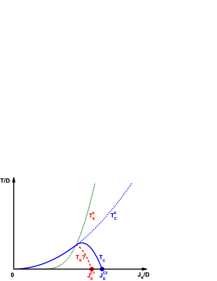
Figure 1: (Color online) The schematic phase diagram expected from the interplay between ferromagnetic correlations and the Kondo screening effect. $T_{C}^{0}$ denotes the Curie temperature in the absence of the Kondo effect, and $T_{K}^{0}$ represents the Kondo temperature without the ferromagnetic correlations.

In our previous paper,Li-Zhang-Yu we have carefully studied the possible ground state phases within an effective mean field theory. In particular, for $0.16<n_{c}<0.82$ and close to the magnetic phase transition, the local moments can be only partially screened by the conduction electrons, and the remaining uncompensated parts develop the ferromagnetic long-range order. Depending on the Kondo coupling strength, the resulting ground state is either a spin fully polarized or a partially polarized ferromagnetic phase according to the quasiparticles around the Fermi energy. The existence of the spin fully polarized coexistent Kondo ferromagnetic phase has been confirmed by the recent dynamic mean-field calculations in infinite dimensions and density matrix renormalization group in one dimension, where such a state is referred to as the spin-selective Kondo insulator.Peters-2012

In the present paper, we will derive a similar finite temperature phase diagram of the Kondo lattice model to Fig.1 for small conduction electron densities. Below the Curie temperature, we find a characteristic temperature scale to signal the Kondo screening effect for the first time. Moreover, there exist a spin fully polarized phase and a partially polarized ferromagnetic long-range ordered phase coexisting with the Kondo screening effect. The former phase spans a large area in the phase diagram, while the latter phase just occupies a very narrow region close to the phase boundary of the paramagnetic heavy Fermi liquid phase. Moreover, a second order phase transition occurs from the spin partially polarized ferromagnetic ordered state to the paramagnetic heavy Fermi liquid state, and the transition line becomes very steep close to the quantum critical point. Our results may be used to explain the weak ferromagnetism and quantum critical behavior observed in YbNi₄P₂.Krellner-2011

The Hamiltonian of the Kondo lattice systems is defined by

$$\mathcal{H}=\sum_{\mathbf{k},{\sigma}}\epsilon_{\mathbf{k}}c_{\mathbf{k}\sigma}^{\dagger}c_{\mathbf{k}\sigma}+J_{K}\sum_{i}\mathbf{\sigma}_{i}\cdot\mathbf{S}_{i},$$ (1)

where $\epsilon_{\mathbf{k}}$ is the dispersion of the conduction electrons, $\mathbf{\sigma}_{i}=\frac{1}{2}\sum_{{\alpha}\beta}c_{i\alpha}^{\dagger}\mathbf{\tau}_{\alpha\beta}c_{i\beta}$ is the spin density operator of the conduction electrons, $\mathbf{\tau}$ is the Pauli matrix, and the Kondo coupling strength $J_{K}>0$. When the localized spins are denoted by $\mathbf{S}_{i}=\frac{1}{2}\sum_{{\alpha}\beta}f_{i\alpha}^{\dagger}\mathbf{\tau}_{\alpha\beta}f_{i\beta}$ in the pseudo-fermion representation, the projection onto the physical subspace has to be implemented by a local constraint $\sum_{\sigma}f_{i\sigma}^{\dagger}f_{i\sigma}=1$. It is straightforward to decompose the Kondo spin exchange into longitudinal and transversal parts

$$\mathbf{\sigma}_{i}\cdot\mathbf{S}_{i}=\sigma_{i}^{z}S_{i}^{z}-\frac{1}{4}[(c_{i\uparrow}^{\dagger}f_{i\uparrow}+f_{i\downarrow}^{\dagger}c_{i\downarrow})^{2}+(c_{i\downarrow}^{\dagger}f_{i\downarrow}+f_{i\uparrow}^{\dagger}c_{i\uparrow})^{2}],$$

where the longitudinal part describes the polarization of the conduction electrons, giving rise to the usual RKKY interaction among the local moments; while the transverse part represents the spin-flip scattering of the conduction electrons by the local moments, yielding the local Kondo screening effect.Lacroix1979 ; Zhang2000a The latter effect has been investigated by various approaches, in particular, those based on a $1/N$ expansionread ; coleman ; burdin ($N$ is the degeneracy of the localized spin). However, the competition between these two interactions determines the possible ground states of the Kondo lattice systems.

Let us first review the effective mean field theory for the ground state used in our previous study.Li-Zhang-Yu We introduce two ferromagnetic order parameters: $m_{f}=\left\langle S_{i}^{z}\right\rangle$ and $m_{c}=\langle\sigma_{i}^{z}\rangle$ to decouple the longitudinal exchange term, while a hybridization order parameter $V=\langle c_{i\uparrow}^{\dagger}f_{i\uparrow}+f_{i\downarrow}^{\dagger}c_{i\downarrow}\rangle$ is introduced to decouple the transverse exchange term. We also introduce a Lagrangian multiplier $\lambda$ to enforce the local constraint, which becomes the chemical potential in the mean field approximation. Then the mean field Hamiltonian in the momentum space can be written in a compact form

$$\mathcal{H}_{MF}=\sum_{\mathbf{k},{\sigma}}\left(c_{\mathbf{k}\sigma}^{\dagger},f_{\mathbf{k}\sigma}^{\dagger}\right)\left(\begin{array}[]{cc}\epsilon_{\mathbf{k}{\sigma}}&-\frac{J_{K}V}{2}\\ -\frac{J_{K}V}{2}&\lambda_{{\sigma}}\end{array}\right)\left(\begin{array}[]{c}c_{\mathbf{k}\sigma}\\ f_{\mathbf{k}\sigma}\end{array}\right)+\mathcal{N}\varepsilon_{0},$$ (2)

where $\epsilon_{\mathbf{k}{\sigma}}=\epsilon_{\mathbf{k}}+\frac{J_{K}m_{f}}{2}{\sigma}$, $\lambda_{{\sigma}}=\lambda+\frac{J_{K}m_{c}}{2}{\sigma}$, $\varepsilon_{0}=\frac{J_{K}V^{2}}{2}-J_{K}m_{c}m_{f}-\lambda$, ${\sigma=\pm 1}$ denote the up and down spin orientations, and $\mathcal{N}$ is the total number of lattice sites. The quasiparticle excitation spectra are thus obtained by

$$E_{\mathbf{k}{\sigma}}^{\pm}=\frac{1}{2}\left[\epsilon_{\mathbf{k}{\sigma}}+\lambda_{{\sigma}}\pm\sqrt{\left(\epsilon_{\mathbf{k}{\sigma}}-\lambda_{{\sigma}}\right)^{2}+(J_{K}V)^{2}}\right],$$ (3)

where there appear four quasiparticle bands with spin splitting.

Using the method of equation of motion, the single particle Green functions can be derived, while the corresponding density of states can be calculated and expressed as

$$\rho_{c}^{\sigma}(\omega)=\rho_{c}^{0}[\theta(\omega-\omega_{1\sigma})\theta(\omega_{2\sigma}-\omega)+\theta(\omega-\omega_{3\sigma})\theta(\omega_{4\sigma}-\omega)],$$

$$\rho_{f}^{\sigma}(\omega)=\left(\frac{J_{K}V/2}{\omega-\lambda_{{\sigma}}}\right)^{2}\rho_{c}^{\sigma}(\omega),$$ (4)

where $\theta(\omega)$ is a step function and a constant density of states of conduction electrons has been assumed $\rho_{c}^{0}=\frac{1}{2D}$, with $D$ as a half-width of the conduction electron band. The four quasiparticle band edges can be expressed as

$$\omega_{1\sigma} =\frac{1}{2}\left[\epsilon_{\sigma}-D+\lambda_{{\sigma}}-\sqrt{(\epsilon_{\sigma}-D-\lambda_{{\sigma}})^{2}+(J_{K}V)^{2}}\right],$$

$$\omega_{2\sigma} =\frac{1}{2}\left[\epsilon_{\sigma}+D+\lambda_{{\sigma}}-\sqrt{(\epsilon_{\sigma}+D-\lambda_{{\sigma}})^{2}+(J_{K}V)^{2}}\right],$$

$$\omega_{3\sigma} =\frac{1}{2}\left[\epsilon_{\sigma}-D+\lambda_{{\sigma}}+\sqrt{(\epsilon_{\sigma}-D-\lambda_{{\sigma}})^{2}+(J_{K}V)^{2}}\right],$$

$$\omega_{4\sigma} =\frac{1}{2}\left[\epsilon_{\sigma}+D+\lambda_{{\sigma}}+\sqrt{(\epsilon_{\sigma}+D-\lambda_{{\sigma}})^{2}+(J_{K}V)^{2}}\right],$$

where $\epsilon_{\sigma}=\frac{J_{K}m_{f}}{2}{\sigma}$ and $\omega_{1\sigma}<\omega_{2\sigma}<\omega_{3\sigma}<\omega_{4\sigma}$.

Then using the spectral representation of the Green functions, we derive the mean-field equations at finite temperatures as follows

$$\int_{-\infty}^{+\infty}d\omega f(\omega)\left[\rho_{c}^{+}(\omega)+\rho_{c}^{-}(\omega)\right] = n_{c},$$

$$\int_{-\infty}^{+\infty}d\omega f(\omega)\left[\rho_{c}^{+}(\omega)-\rho_{c}^{-}(\omega)\right] = 2m_{c},$$

$$\sum\limits_{\sigma}\int_{-\infty}^{+\infty}d\omega f(\omega)\frac{\rho_{c}^{\sigma}(\omega)}{\left(\lambda_{\sigma}-\omega\right)^{2}}\left(\frac{J_{K}V}{2}\right)^{2} = 1,$$

$$\sum\limits_{\sigma}\int_{-\infty}^{+\infty}d\omega f(\omega)\frac{\sigma\rho_{c}^{\sigma}(\omega)}{\left(\lambda_{\sigma}-\omega\right)^{2}}\left(\frac{J_{K}V}{2}\right)^{2} = 2m_{f},$$

$$\sum\limits_{\sigma}\int_{-\infty}^{+\infty}d\omega f(\omega)\frac{\rho_{c}^{\sigma}(\omega)}{\left(\lambda_{\sigma}-\omega\right)}\left(\frac{J_{K}V}{2}\right) = V,$$ (5)

where $f(\omega)=1/\left[1+e^{(\omega-\mu)/T}\right]$ is the Fermi distribution function. To make the magnetic interaction between the nearest neighboring local moments ferromagnetic, we should confine the density of conduction electrons to $n_{c}<0.82$ from the previous mean field study.Fazekas1991

The position of the chemical potential $\mu$ with respect to the band edges is very important. At zero temperature, there are two different situations. The corresponding schematic local density of states are displayed in Fig.2. For $\omega_{1-}<\mu<\omega_{2+}$, both the lower spin-up and spin-down quasiparticle bands are partially occupied, corresponding to the spin partially polarized ferromagnetic state. However, for $\omega_{2+}<\mu<\omega_{2-}$, the lower spin-up quasiparticle band is completely occupied, while the lower spin-down quasiparticle band is only partially occupied, corresponding to the spin fully polarized ferromagnetic state.Beach-Assaad An energy gap $\Delta_{\uparrow}$ exists in the spin-up quasiparticle band, and there is a plateau in the total magnetization: $m_{c}+m_{f}=(1-n_{c})/2$.

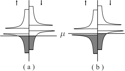
Figure 2: Schematic DOS in the presence of Kondo screening effect. (a) for the spin partially polarized ferromagnetic phase, (b) for the spin fully polarized ferromagnetic phase.

The ground-state phase diagram has been obtained in our previous study.Li-Zhang-Yu When $n_{c}<0.16$, the spin-polarized ferromagnetic phase is a ground state in the large Kondo coupling region. For $0.16<n_{c}<0.82$, the ground state is given by the spin partially polarized ferromagnetic phase in the weak Kondo coupling limit; while in the intermediate Kondo coupling regime, both spin fully polarized and partially polarized ferromagnetic ordered phases with a finite value of the hybridization parameter $V$ may appear, depending on the value of the Kondo coupling strength. For a strong Kondo coupling, the pure Kondo paramagnetic phase is the ground state. There is a continuous transition from the spin partially polarized ferromagnetic ordered phase to the Kondo paramagnetic phase.

Now we calculate the finite temperature phase diagram. First of all, if the temperature is high enough, all order parameters must disappear, so the conduction electrons and local moments are decoupled. As the temperature is decreased down to the Curie temperature of the pure ferromagnetic phase $T_{C}^{0}$, both $m_{c}$ and $m_{f}$ approach zero, but the ratio $m_{c}/m_{f}$ is finite. The self-consistent equations give rise to

$$\lambda=\mu,m_{c}\approx-\frac{J_{K}}{4D}m_{f},m_{f}=-\frac{J_{K}}{8T_{C}^{0}}m_{c},$$ (6)

and the Curie temperature $T_{C}^{0}$ can be estimated as

$$T_{C}^{0}=\frac{J_{K}^{2}}{32D},$$ (7)

which is independent of the density of conduction electrons, similar to the characteristic energy scale given by the RKKY interaction.

On the other hand, if $J_{K}$ is large enough, the system must be in the Kondo paramagnetic phase. As the Kondo coupling decreases, the Kondo singlets are destabilized. When $T\rightarrow T_{K}^{0}$, the hybridization vanishes, and the self-consistent equations can be reduced to

$$\frac{1}{D}\int\limits_{-D}^{D}\frac{d\omega}{e^{(\omega-\mu)/T_{K}^{0}}+1} = n_{c},$$

$$\frac{J_{K}}{2D}\int\limits_{-D}^{D}d\omega\frac{\tanh(\frac{\omega-\mu}{T_{K}^{0}})}{\omega-\mu} = 1.$$ (8)

When we numerically solve these two equations, the Kondo temperature in the paramagnetic phase $T_{K}^{0}$ can be obtained, which is the same characteristic energy scale as derived from the $1/N$ expansion.read ; coleman ; burdin

After obtaining $T_{C}^{0}$ and $T_{K}^{0}$, we expect that the pure ferromagnetic phase exists for $T_{C}^{0}>T_{K}^{0}$ in the small Kondo coupling limit, while for $T_{K}^{0}>T_{C}^{0}$ the Kondo screening is present, and the competition between the ferromagnetic correlations and Kondo screening effect should be taken into account more carefully.

In the presence of the Kondo screening, the corresponding Curie temperature $T_{C}$ can be still defined. As $T\rightarrow T_{C}$, the magnetic moments $m_{c}$ and $m_{f}$ approach zero, but their ratio is finite, $m_{c}/m_{f}\neq 0$. The self-consistent equations Eq.(5) can be solved numerically, leading to the Curie temperature $T_{C}$ and the mean-field parameters of $\mu$, $\lambda$, $V$, and $m_{c}/m_{f}$. On the other hand, when the ferromagnetism is present, we can also introduce the Kondo temperature $T_{K}$ incorporating the hybridization effect. When $V\rightarrow 0$ and $T\rightarrow T_{K}$, the numerical solution of the self-consistent equations gives rise to the Kondo temperature $T_{K}$ and the mean-field parameters $\mu$, $\lambda$, $m_{c}$, and $m_{f}$.

The resulting phase diagram is shown in Fig.3 for $n_{c}=0.2$. As the Kondo coupling $J_{K}$ increases from a small value, the Curie temperature $T_{C}$ first increases up to a maximal value, and then continuously decreases to zero at $J_{K}^{c2}=1.133D$. For small values of $J_{K}/D<0.41$, the Kondo temperature $T_{K}$ vanishes. However, when $J_{K}/D>0.41$, the Kondo temperature curve consists of two parts, meeting each other precisely at the Curie temperature ($T_{K}=T_{C}$). Inside the ferromagnetic ordered phase, $T_{K}$ starts from a finite value and then decreases down to zero at $J_{K}^{c1}=0.506D$; while in the paramagnetic phase, $T_{K}$ follows the behavior of the bare Kondo temperature $T_{K}^{0}$.

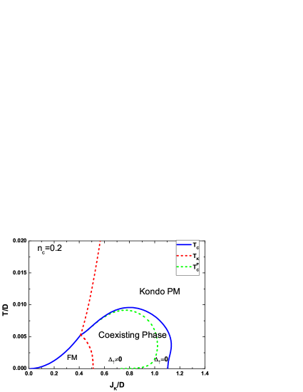
Figure 3: (Color online) The finite temperature phase diagram at $n_{c}=0.2$. In addition to the pure ferromagnetic ordered phase ($V=0$, $m_{c}\neq 0$ and $m_{f}\neq 0$) and the Kondo paramagnetic phase ($V\neq 0$, $m_{c}=m_{f}=0$), there are two different ferromagnetic ordered phases coexisting with the Kondo screening ($V\neq 0$, $m_{c}\neq 0$ and $m_{f}\neq 0$): the spin fully polarized phase ($\Delta_{\uparrow}\neq 0$) and spin partially polarized phase ($\Delta_{\uparrow}=0$). The boundary of the pure ferromagnetic order phase and the coexisting ferromagnetic ordered phases actually corresponds to a crossover not a phase transition.

In the coexistence region, depending on whether the chemical potential $\mu$ is inside the energy gap of spin-up quasi-particle (as shown in Fig.2), we can calculate the lowest excitation energy defined by $\Delta_{\uparrow}\equiv\mu-\omega_{2+}$. In Fig.4, we show $\Delta_{\uparrow}$ as a function of $T$ with fixed Kondo coupling parameters $J_{K}/D=0.6$, $0.7$, $0.733$, $0.9$ and $1.0$, respectively. It is clearly demonstrated that the gap $\Delta_{\uparrow}$ has a non-monotonic behavior as the temperature increases. Notice that $J_{K}/D=0.733$ corresponds to the critical value between the spin fully polarized phase and partially polarized phase at zero temperature. When $\Delta_{\uparrow}\rightarrow 0$, the characteristic temperature $T_{C}^{P}$ is determined, leading to the phase boundary separating the spin fully polarized and the partially polarized ferromagnetic ordered phases. The spin fully polarized ferromagnetic order phase spans a large area in the coexistence region, while the spin partially polarized phase just sits in a narrow strip close to the phase boundary of the paramagnetic heavy Fermi liquid phase. The existence of the partially polarized ferromagnetic order phase can be expected before the system enters into the paramagnetic metallic phase.

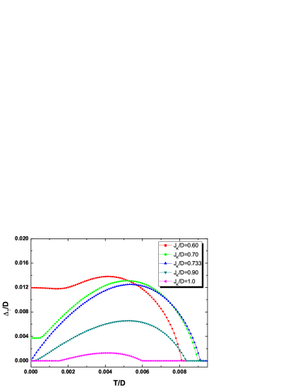
Figure 4: (Color online) The energy gap of spin-up quasiparticles $\Delta_{\uparrow}$ as a function of temperature $T$ in the coexisting phase at $n_{c}=0.2$.

Moreover, the magnetizations of the local moments and the conduction electrons $m_{f}$ and $m_{c}$ are calculated as a function of the Kondo coupling strength $J_{K}$ for $T=0.0025D$ and $0.0075D$, as shown in Fig.5., respectively. It is clear that $m_{c}$ has an opposite sign of $m_{f}$, due to the antiferromagnetic coupling between the local moments and conduction electrons. In order to display the Kondo screening effect, we have also plotted the hybridization parameter $V$ as a function of $J_{K}$ for the same fixed temperatures. For low temperatures shown in Fig.5a, the Kondo screening effect emerges inside the ferromagnetic ordered phase, and a small drop is induced in both magnetizations $m_{f}$ and $m_{c}$. When the magnetization vanishes, the hybridization $V$ has a cusp. However, for high temperatures shown in Fig.5b, the ferromagnetic ordering appears inside the Kondo screened region. The cusps in the hybridization curve are induced when the ferromagnetic order parameters start to emergence or vanish.

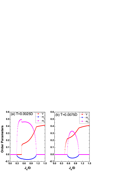
Figure 5: (Color online) The ferromagnetic magnetizations and hybridization parameters as a function of the Kondo coupling $J_{K}$ with a fixed temperature at $n_{c}=0.2$. (a) $T=0.0025D$, (b) $T=0.0075D$.

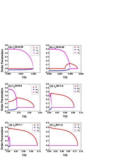
Figure 6: (Color online) The magnetizations and hybridization parameter as a function of temperature for a given Kondo coupling strength at $n_{c}=0.2$. (a), (b), (c), (d), (e), and (f) correspond to $J_{K}/D=0.25$, $0.45$, $0.60$, $1.0$, $1.1$, and $1.2$, respectively.

The magnetizations $m_{c}$ and $m_{f}$ and hybridization parameter $V$ have also been calculated as a function of temperature $T$ for the fixed Kondo coupling strength $J_{K}$, which is shown in Fig.6. For a small value of $J_{K}/D=0.2$, as the temperature is increased, the magnetic moments $m_{c}$ and $m_{f}$ in the absence of the Kondo screening decrease down to zero at the Curie temperature $T_{C}$ (see Fig.6a). In contrast, for a large value of $J_{K}/D=1.2$, the system is in a paramagnetic heavy Fermi liquid phase without ferromagnetic order (see Fig.6f).

For $J_{K}/D=0.45$, the Kondo screening effect starts to appear in the presence of ferromagnetic ordering. When the ferromagnetic order disappears at $T_{C}$, the hybridization reaches a maximal value and then decreases down to zero at $T_{K}$ (see Fig.6b). For larger values of the Kondo coupling $J_{K}/D=0.6$, $1.0$, and $1.1$, the Kondo screening effect dominates in the temperature range, and the ferromagnetic ordering phase occurs only in a small region, displayed in Fig.6c, Fig.6d and Fig.6e, respectively. These three figures demonstrate the interplay between the Kondo screening effect and the ferromagnetic correlations in the presence of thermal fluctuations.

It is important to emphasize that all the results are obtained within the effective mean field theory. When the fluctuation effects are incorporated properly beyond the mean field level, the above phase transitions related to the Kondo screening effect will be changed into a crossover. Since the Kondo screening order parameter, i.e. the effective hybridization is not associated with a static long-range order, the finite $V$ does not correspond to any spontaneous symmetry breaking. Therefore, in the obtained finite temperature phase diagram Fig.3, only the Curie temperature $T_{C}$ (the solid line) represents a true phase transition.

Finally, it is important to mention a new Kondo lattice system YbNi₄P₂, recently discovered by distinct anomalies in susceptibility, specific heat and resistivity measurements.Krellner-2011 Growing out of a strongly correlated Kramers doublet ground state with Kondo temperature $T_{K}\sim 8K$, the ferromagnetic ordering temperature is severely reduced to $T_{c}=0.17$K with a small magnetic moment $m_{f}\sim 0.05\mu_{B}$. Here we would like to explain the small ferromagnetically order moment and the substantially reduced Curie temperature as originating from the presence of the Kondo screening effect, see Fig.6c, Fig.6d, and Fig.6e. The experimental results can certainly be understood in terms of our effective mean field theory. The quantum critical behavior observed experimentally requires a quantum critical point separating the ferromagnetic ordered phase from the Kondo paramagnetic phase at zero temperature, which is also consistent with our finite temperature phase diagram. The further detailed calculations concerning with thermodynamic properties of the heavy fermion ferromagnetism are left for our future research.

In summary, within an effective mean-field theory for small conduction electron densities $0.16<n_{c}<0.82$, we have derived the finite temperature phase diagram. Inside the ferromagnetic ordered phase, a characteristic temperature scale has been found to signal the Kondo screening effect for the first time. In additional to the pure ferromagnetic phase, there are two distinct ferromagnetic long-range ordered phases coexisting with the Kondo screening effect: a spin fully polarized phase and a partially polarized phase. A second-order phase transition and a quantum critical point have been found to separate the spin partially polarized ferromagnetic ordered phase and the paramagnetic heavy Fermi liquid phase. To some extent, our mean field theory has captured the main physics of the Kondo lattice systems, which provides an alternative interpretation of weak ferromagnetism observed experimentally.

The authors acknowledge the support from NSF-China.

Note added. The ferromagnetic quantum critical point in the heavy fermion metal YbNi₄(P_0.92As_0.08)₂ has been further confirmed Steppke by precision low temperature measurements: the Gruneisen ratio diverges upon cooling to $T=0K$.

References

- (1) G. R. Stewart, Rev. Mod. Phys. 73, 797 (2001).
- (2) H. v. Lohneysen, A. Rosch, M. Vojta, and P. Wölfle, Rev. Mod. Phys. 79, 1015 (2007).
- (3) Q. Si and F. Steglich, Science 329, 1161 (2010).
- (4) S. Doniach, Physica, B & C 91, 231 (1977).
- (5) C. Lacroix, and M. Cyrot, Phys. Rev. B 20, 1969 (1979).
- (6) Q. Si, Physica B 378, 23 (2006); Phys. Status Solidi, B 247, 476 (2010).
- (7) G. M. Zhang and L. Yu, Phys. Rev. B 62, 76 (2000).
- (8) S. Capponi and F. F. Assaad, Phys. Rev. B 63, 155114 (2001).
- (9) H. Watanabe and M. Ogata, Phys. Rev. Lett. 99, 136401 (2007).
- (10) L. C. Martin and F. F. Assaad, Phys. Rev. Lett. 101, 066404 (2008).
- (11) O. O. Bernal, D. E. MacLaughlin, H. G. Lukefahr, and B. Andraka, Phys. Rev. Lett. 75, 2023 (1995).
- (12) N. T. Huy, et al., Phys. Rev. B 75, 212405 (2007).
- (13) C. Krellner, et al., New J. Phys. 13, 103014 (2011).
- (14) A. Fernandez-Panella, D. Braithwaite, B. Salce, G. Lapertot, and J. Flouquet, Phys. Rev. B 84, 134416 (2011).
- (15) S. Lausberg, et al., arXiv:1210.1345.
- (16) V. Y. Irkhin and M. I. Katsnelson, Z. Phys. B 82, 77 (1991).
- (17) M. Sigrist, K. Ueda, and H. Tsunetsugu, Phys. Rev. B 46, 175 (1992).
- (18) Z. Z. Li, M. Zhuang, and M. W. Xiao, J. Phys.: Condens. Matter 8 7941 (1996).
- (19) S. J. Yamamoto and Q. Si, Proc. Nat. Acad. Sci. 107, 15704 (2010).
- (20) G. B. Li, G. M. Zhang, and L. Yu, Phys. Rev. B 81, 094420 (2010).
- (21) R. Peters, N. Kawakami, and T. Pruschke, Phys. Rev. Lett. 108, 086402 (2012); R. Peters and N. Kawakami, Phys. Rev. B 86, 165107 (2012).
- (22) N. Read and D. N. Newns, J. Phys. C 16, 3273 (1983).
- (23) P. Coleman, Phys. Rev. B 29, 3035 (1984).
- (24) S. Burdin, A. Georges, and D. R. Grempel, Phys. Rev. Lett. 85, 1048 (2000).
- (25) P. Fazekas and E. Müller-Hartmann, Z. Phys. B 85, 285 (1991).
- (26) K. S. D. Beach and F. F. Assaad, Phys. Rev. B 77, 205123 (2008); S. Viola Kusminskiy, K. S. D. Beach, A. H. Castro Neto, and D. K. Campbell, Phys. Rev. B 77, 094419 (2008).
- (27) A. Steppke, et al., Science 339, 933 (2013).