Quantum Robust Stability of a Small Josephson Junction in a Resonant Cavity

Abstract

This paper applies recent results on the robust stability of nonlinear quantum systems to the case of a Josephson junction in a resonant cavity. The Josephson junction is characterized by a Hamiltonian operator which contains a non-quadratic term involving a cosine function. This leads to a sector bounded nonlinearity which enables the previously developed theory to be applied to this system in order to analyze its stability.

I Introduction

In recent years, a number of papers have considered the feedback control of systems whose dynamics are governed by the laws of quantum mechanics rather than classical mechanics; e.g., see [1, 2, 3, 4, 5, 6, 7, 8, 9, 10, 11, 12, 13]. In particular, the papers [10, 14] consider a framework of quantum systems defined in terms of a triple $(S,L,H)$ where $S$ is a scattering matrix, $L$ is a vector of coupling operators and $H$ is a Hamiltonian operator.

The paper [15] considers the problem of absolute stability for a quantum system defined in terms of a triple $(S,L,H)$ in which the quantum system Hamiltonian is decomposed as $H=H_{1}+H_{2}$ where $H_{1}$ is a known nominal Hamiltonian and $H_{2}$ is a perturbation Hamiltonian, which is contained in a specified set of Hamiltonians $\mathcal{W}$. In particular the paper [15] considers the case in which the nominal Hamiltonian $H_{1}$ is a quadratic function of annihilation and creation operators and the coupling operator vector is a linear function of annihilation and creation operators. This case corresponds to a nominal linear quantum system; e.g., see [4, 5, 7, 8, 13]. Also, it is assumed that $H_{2}$ is contained in a set of non-quadratic perturbation Hamiltonians corresponding to a sector bound on the nonlinearity In this special case, [15] obtains a robust stability result in terms of a frequency domain condition.

In this paper, we apply the result of [15] to a quantum system which consists of a Josephson junction in a resonant cavity as described in the paper [16]. This enables us to analyze the stability of this quantum system. In particular, this enables us to choose suitable values for the coupling parameters in the system. For the parameter values chosen, we show that the quantum system is robustly mean square stable according to the definition of [15].

II Quantum Systems

The main result of the paper [15] considers open quantum systems defined by parameters $(S,L,H)$ where $H=H_{1}+H_{2}$; e.g., see [10, 14]. The corresponding generator for this quantum system is given by

$$\mathcal{G}(X)=-i[X,H]+\mathcal{L}(X)$$ (1)

where $\mathcal{L}(X)=\frac{1}{2}L^{\dagger}[X,L]+\frac{1}{2}[L^{\dagger},X]L$. Here, $[X,H]=XH-HX$ denotes the commutator between two operators and the notation ^† denotes the adjoint transpose of a vector of operators. Also, $H_{1}$ is a self-adjoint operator on the underlying Hilbert space referred to as the nominal Hamiltonian and $H_{2}$ is a self-adjoint operator on the underlying Hilbert space referred to as the perturbation Hamiltonian. The triple $(S,L,H)$, along with the corresponding generators define the Heisenberg evolution $X(t)$ of an operator $X$ according to a quantum stochastic differential equation; e.g., see [14].

We now define a set of non-quadratic perturbation Hamiltonians denoted $\mathcal{W}$. The set $\mathcal{W}$ is defined in terms of the following power series (which is assumed to converge in the sense of the induced operator norm on the underlying Hilbert space)

$$H_{2}=f(\zeta,\zeta^{*})=\sum_{k=0}^{\infty}\sum_{\ell=0}^{\infty}S_{k\ell}\zeta^{k}(\zeta^{*})^{\ell}=\sum_{k=0}^{\infty}\sum_{\ell=0}^{\infty}S_{k\ell}H_{k\ell}.$$ (2)

Here $S_{k\ell}=S_{\ell k}^{*}$, $H_{k\ell}=\zeta^{k}(\zeta^{*})^{\ell}$, and $\zeta$ is a scalar operator on the underlying Hilbert space. Also, ^∗ denotes the adjoint of a scalar operator. It follows from this definition that

$$H_{2}^{*}=\sum_{k=0}^{\infty}\sum_{\ell=0}^{\infty}S_{k\ell}^{*}\zeta^{\ell}(\zeta^{*})^{k}=\sum_{\ell=0}^{\infty}\sum_{k=0}^{\infty}S_{\ell k}\zeta^{\ell}(\zeta^{*})^{k}=H_{2}$$

and thus $H_{2}$ is a self-adjoint operator. Note that it follows from the use of Wick ordering that the form (2) is the most general form for a perturbation Hamiltonian defined in terms of a single scalar operator $\zeta$.

Also, we let

$$f^{\prime}(\zeta,\zeta^{*})=\sum_{k=1}^{\infty}\sum_{\ell=0}^{\infty}kS_{k\ell}\zeta^{k-1}(\zeta^{*})^{\ell},$$ (3)

$$f^{\prime\prime}(\zeta,\zeta^{*})=\sum_{k=1}^{\infty}\sum_{\ell=0}^{\infty}k(k-1)S_{k\ell}\zeta^{k-2}(\zeta^{*})^{\ell}$$ (4)

and consider the sector bound condition

$$f^{\prime}(\zeta,\zeta^{*})^{*}f^{\prime}(\zeta,\zeta^{*})\leq\frac{1}{\gamma^{2}}\zeta\zeta^{*}+\delta_{1}$$ (5)

and the condition

$$f^{\prime\prime}(\zeta,\zeta^{*})^{*}f^{\prime\prime}(\zeta,\zeta^{*})\leq\delta_{2}.$$ (6)

Then we define the set $\mathcal{W}$ as follows:

$$\mathcal{W}=\left\{\begin{array}[]{l}H_{2}\mbox{ of the form (\ref{H2nonquad}) such that }\\ \mbox{ conditions (\ref{sector4a}) and (\ref{sector4b}) are satisfied}\end{array}\right\}.$$ (7)

Reference [15] also considers the case in which the nominal quantum system corresponds to a linear quantum system; e.g., see [4, 5, 7, 8, 13]. In this case, $H_{1}$ is of the form

$$H_{1}=\frac{1}{2}\left[\begin{array}[]{cc}a^{\dagger}&a^{T}\end{array}\right]M\left[\begin{array}[]{c}a\\ a^{\#}\end{array}\right]$$ (8)

where $M\in\mathbb{C}^{2n\times 2n}$ is a Hermitian matrix of the form

$$M=\left[\begin{array}[]{cc}M_{1}&M_{2}\\ M_{2}^{\#}&M_{1}^{\#}\end{array}\right]$$ (9)

and $M_{1}=M_{1}^{\dagger}$, $M_{2}=M_{2}^{T}$. Here, the notation ^# denotes the vector of adjoint operators for a vector of operators. Also, ^# denotes denotes the complex conjugate of a matrix for a complex matrix. In addition, we assume $L$ is of the form

$$L=\left[\begin{array}[]{cc}N_{1}&N_{2}\end{array}\right]\left[\begin{array}[]{c}a\\ a^{\#}\end{array}\right]$$ (10)

where $N_{1}\in\mathbb{C}^{m\times n}$ and $N_{2}\in\mathbb{C}^{m\times n}$. Also, we write

$$\left[\begin{array}[]{c}L\\ L^{\#}\end{array}\right]=N\left[\begin{array}[]{c}a\\ a^{\#}\end{array}\right]=\left[\begin{array}[]{cc}N_{1}&N_{2}\\ N_{2}^{\#}&N_{1}^{\#}\end{array}\right]\left[\begin{array}[]{c}a\\ a^{\#}\end{array}\right].$$

As in [15], we consider a notion of robust mean square stability.

Definition 1

An uncertain open quantum system defined by $(S,L,H)$ where $H=H_{1}+H_{2}$ with $H_{1}$ of the form (8), $H_{2}\in\mathcal{W}$, and $L$ of the form (10) is said to be robustly mean square stable if for any $H_{2}\in\mathcal{W}$, there exist constants $c_{1}>0$, $c_{2}>0$ and $c_{3}\geq 0$ such that

$$\left<\left[\begin{array}[]{c}a(t)\\ a^{\#}(t)\end{array}\right]^{\dagger}\left[\begin{array}[]{c}a(t)\\ a^{\#}(t)\end{array}\right]\right>$$ (15)

$$\leq c_{1}e^{-c_{2}t}\left<\left[\begin{array}[]{c}a\\ a^{\#}\end{array}\right]^{\dagger}\left[\begin{array}[]{c}a\\ a^{\#}\end{array}\right]\right>+c_{3}~{}~{}\forall t\geq 0.$$ (20)

Here $\left[\begin{array}[]{c}a(t)\\ a^{\#}(t)\end{array}\right]$ denotes the Heisenberg evolution of the vector of operators $\left[\begin{array}[]{c}a\\ a^{\#}\end{array}\right]$; e.g., see [14].

We define

$$\zeta = E_{1}a+E_{2}a^{\#}$$ (26)

$$= \left[\begin{array}[]{cc}E_{1}&E_{2}\end{array}\right]\left[\begin{array}[]{c}a\\ a^{\#}\end{array}\right]=\tilde{E}\left[\begin{array}[]{c}a\\ a^{\#}\end{array}\right]$$

where $\zeta$ is a scalar operator. Then, the following following strict bounded real condition provides a sufficient condition for the robust mean square stability of the nonlinear quantum system under consideration when $H_{2}\in\mathcal{W}$:

1. The matrix

   $$F=-iJM-\frac{1}{2}JN^{\dagger}JN\mbox{ is Hurwitz;}$$ (27)

2. $$\left\|\tilde{E}^{\#}\Sigma\left(sI-F\right)^{-1}\tilde{D}\right\|_{\infty}<\frac{\gamma}{2}$$ (28)

   where

   $$\tilde{D} = J\Sigma\tilde{E}^{T},$$

   $$J = \left[\begin{array}[]{cc}I&0\\ 0&-I\end{array}\right],$$

   $$\Sigma = \left[\begin{array}[]{cc}0&I\\ I&0\end{array}\right].$$

This leads to the following theorem which is presented in [15].

Theorem 1

Consider an uncertain open quantum system defined by $(S,L,H)$ such that $H=H_{1}+H_{2}$ where $H_{1}$ is of the form (8), $L$ is of the form (10) and $H_{2}\in\mathcal{W}$. Furthermore, assume that the strict bounded real condition (27), (28) is satisfied. Then the uncertain quantum system is robustly mean square stable.

In the next section, we will apply this theorem to analyze the stability of a nonlinear quantum system corresponding to a Josephson junction in a resonant cavity.

III The Josephson Junction in a Resonant Cavity System

We consider a quantum system consisting of a small Josephson junction coupled to an electromagnetic resonant cavity. This system has been considered in the paper [16] where a Hamiltonian for the system is derived. The paper [16] considers the system as a closed quantum system defined purely in terms of a system Hamiltonian. We modify this description of the system to consider an open quantum system model which interacts with external fields by introducing coupling operators for the system in order to apply the results of [15] given above. The coupling operator which is introduced is taken as a standard coupling operator for a resonant cavity coupled to a single field as well as a corresponding coupling operator for the Josephson junction coupled to an external heat bath.

A Josephson junction consists of a thin insulating material between two superconducting layers. As in [16], we consider a Josephson junction in a resonant cavity. This is illustrated in Figure 1.

Figure 1: Schematic diagram of a Josephson junction in a resonant cavity.

The following Hamiltonian for the Josephson junction system is derived in [16]

$$\mathcal{H} = \frac{1}{2\hbar}U^{\prime}(n^{\prime}-\bar{n}^{\prime})^{2}-\frac{J^{\prime}}{\hbar}\cos\phi^{\prime}+\frac{1}{2\hbar}(p^{\prime 2}+\omega^{2}q^{\prime 2})$$ (31)

$$-g\sqrt{\frac{\omega}{\hbar}}p^{\prime}n^{\prime}+\frac{U\omega\bar{n}^{2}g^{2}}{2U^{\prime}}$$

where $\bar{n}^{\prime}=\frac{U\bar{n}}{U^{\prime}}$, $U^{\prime}=U+\hbar\omega g^{2}$, $[\phi^{\prime},n^{\prime}]=i$, and $[q^{\prime},p^{\prime}]=i\hbar$. Here

$$\phi^{\prime} = \phi-g\sqrt{\omega/\hbar}q,\quad n^{\prime}=n$$

$$p^{\prime} = p+g\sqrt{\omega\hbar}n,\quad q^{\prime}=q$$

where $q$ and $p$ are the position and momentum operators for the resonant cavity. Also, $n$ is an operator which represents the difference between the number of Cooper pairs on the two superconducting islands which make up the junction. Furthermore, $\phi$ is an operator which represents the phase difference across the junction. Note that compared to the expression for the Hamiltonian given in [16], we have normalized the expression (31) by dividing through by a factor of $\hbar$ in order to be consistent with the convention used in [15].

The quantities $U$, $J^{\prime}$, $\bar{n}$, $g$, $\omega$ are physical constants associated with the junction and the resonant cavity. In particular, $U$ is the charging energy of the Josephson junction, $J^{\prime}$ is the Josephson energy of the junction, $\bar{n}$ is an experimental parameter relating to the gate voltage applied to the superconducting islands, $g$ is a parameter related to the dimensions of the junction, and $\omega$ is an angular frequency related to the detuning of the cavity; see [16].

By a process of completion of squares, defining new variables $n^{\prime\prime}=n^{\prime}-\bar{n}$, $p^{\prime\prime}=p^{\prime}-g\sqrt{\hbar\omega}$ and neglecting the constant terms, we can re-write the Hamiltonian as follows:

$$\mathcal{H}^{\prime}=$$

$$\frac{1}{2}[q^{\prime}~{}p^{\prime\prime}~{}n^{\prime\prime}~{}\phi^{\prime}]\left[\begin{array}[]{cccc}\frac{\omega^{2}}{\hbar}&0&0&0\\ 0&\frac{1}{\hbar}&-g\sqrt{\frac{\omega}{\hbar}}&0\\ 0&-g\sqrt{\frac{\omega}{\hbar}}&\frac{U^{\prime}}{\hbar}&0\\ 0&0&0&0\end{array}\right]\left[\begin{array}[]{c}q^{\prime}\\ p^{\prime\prime}\\ n^{\prime\prime}\\ \phi^{\prime}\end{array}\right]$$

$$-\frac{J^{\prime}}{\hbar}\cos\phi^{\prime}.$$

Now we define new operators $a_{1}=(\omega q^{\prime}+ip^{\prime\prime})/\sqrt{2\hbar\omega}$, and $a_{2}=(\phi^{\prime}+in^{\prime\prime})/\sqrt{2}$ which satisfy the canonical commutation relations $[a_{1},a_{1}^{*}]=1$ and $[a_{2},a_{2}^{*}]=1$. Then, the Hamiltonian can be re-written in the form

$$H=\frac{1}{2}\left[\begin{array}[]{cc}a^{\dagger}&a^{T}\end{array}\right]M\left[\begin{array}[]{c}a\\ a^{\#}\end{array}\right]-\frac{J^{\prime}}{\hbar}\cos(\frac{a_{2}+a_{2}^{*}}{\sqrt{2}})$$ (33)

where $a=\left[\begin{array}[]{c}a_{1}\\ a_{2}\end{array}\right]$ and $M$ is a Hermitian matrix of the form (9). Note that in order to write the Hamiltonian in this form with the matrix $M$ satisfying (9), it is necessary to apply these canonical commutation relations and neglect further constant terms. Also, the fact that the operators $a_{1}$ and $a_{2}$ commute is used to re-distribute terms within the matrix $M$. (Formally $a_{1}$ and $a_{2}$ are defined on different Hilbert spaces but following the standard convention in quantum mechanics we can extend each operator to the tensor product of the two Hilbert spaces and then these two extended operators will commute with each other.)

We now modify the model of [16] by assuming that the cavity and Josephson modes are coupled to fields corresponding to coupling operators of the form

$$L=\left[\begin{array}[]{c}\sqrt{\kappa_{1}}a_{1}\\ \sqrt{\kappa_{2}}a_{2}\end{array}\right].$$

This modification of the quantum system is necessary in order to obtain a damped quantum system whose stability can be established using the approach of [15] and is quite reasonable for an experimental system which will experience damping in both the electromagnetic cavity and in the Josephson junction circuit.

In order to apply Theorem 1 to analyze the stability of this quantum system, we rewrite (33) as

$$H=H_{1}+H_{2}$$

where $H_{1}=\frac{1}{2}\left[\begin{array}[]{cc}a^{\dagger}&a^{T}\end{array}\right]M\left[\begin{array}[]{c}a\\ a^{\#}\end{array}\right]$ and $H_{2}=-\frac{J^{\prime}}{\hbar}\cos(\frac{a_{2}+a_{2}^{*}}{\sqrt{2}})$. That is, we have a quadratic nominal Hamiltonian and a non-quadratic perturbation Hamiltonian. Then, we define $\zeta=a_{2}/\sqrt{2}$ and

$$f(\zeta,\zeta^{*}) = -\frac{J^{\prime}}{\hbar}\cos(\zeta+\zeta^{*})$$

$$f^{\prime}(\zeta,\zeta^{*}) = \frac{J^{\prime}}{\hbar}\sin(\zeta+\zeta^{*})$$

$$f^{\prime\prime}(\zeta,\zeta^{*}) = \frac{J^{\prime}}{\hbar}\cos(\zeta+\zeta^{*}).$$

From this it follows that

$$f^{\prime}(\zeta,\zeta^{*})^{*}f^{\prime}(\zeta,\zeta^{*})\leq 4\frac{J^{\prime 2}}{\hbar^{2}}\zeta\zeta^{*},\quad f^{\prime\prime}(\zeta,\zeta^{*})^{*}f^{\prime\prime}(\zeta,\zeta^{*})\leq\frac{J^{\prime 2}}{\hbar^{2}}$$

and $\gamma=\frac{\hbar}{2J^{\prime}}$.

The numerical values of the constants $\omega$, $g$, $U$, and $J^{\prime}$ are chosen as in [16] as $\frac{\omega}{2\pi}=100\mbox{GHz}$, $g=0.15$, $U=2.2087\times 10^{-22}$, $J^{\prime}=3.6652\times 10^{11}$. Also, we calculate $\gamma/2=6.8209\times 10^{-13}$. The parameters $\kappa_{1}$ and $\kappa_{2}$ will be chosen using Theorem 1 in order guarantee the robust mean square stability of the quantum system. Indeed, for various values of $\kappa_{1}$ and $\kappa_{2}$, we form the transfer function $G_{\kappa_{1},\kappa_{2}}(s)=E^{\#}\Sigma\left(sI-F\right)^{-1}\tilde{D}$ and calculate its $H_{\infty}$ norm.

The $H_{\infty}$ norm of $G_{\kappa_{1},\kappa_{2}}(s)$ was found to be virtually independent of $\kappa_{1}$ and so a physically reasonable value of $\kappa_{1}=10^{11}$ was chosen. With this value of $\kappa_{1}$, a plot of $\|G_{\kappa_{1},\kappa_{2}}(s)\|_{\infty}$ versus $\kappa_{2}$ is shown in Figure 2.

\psfrag{normG}{$\|G_{\kappa_{1},\kappa_{2}}(s)\|_{\infty}$}\psfrag{K1}{$\kappa_{2}$}\psfrag{gam}{$\frac{\gamma}{2}$}\includegraphics[width=227.62204pt]{F2.eps}

Figure 2: Plot of $\|G_{\kappa_{1},\kappa_{2}}(s)\|_{\infty}$ versus $\kappa_{2}$.

From this plot we can see that stability can be guaranteed for $\kappa_{2}>2.2\times 10^{12}$. Hence, choosing a value of $\kappa_{2}=2.5\times 10^{12}$, it follows that stability of Josephson junction system can be guaranteed using Theorem 1. Indeed, with this value of $\kappa_{2}$, we calculate the matrix $F=-iJM-\frac{1}{2}JN^{\dagger}JN$ and find its eigenvalues to be $-5.0000\times 10^{10}\pm 3.3507\times 10^{3}i$ and $-1.2500\times 10^{12}\pm 1.4842\times 10^{3}i$ which implies that the matrix $F$ is Hurwitz. Also, a magnitude Bode plot of the corresponding transfer function $G_{\kappa_{1},\kappa_{2}}(s)$ is shown in Figure 3 below which implies that $\|G_{\kappa_{1},\kappa_{2}}(s)\|_{\infty}=5.5554\times 10^{-13}<\gamma/2=6.8209\times 10^{-13}$. Hence, using Theorem 1, we conclude that the quantum system is robustly mean square stable.

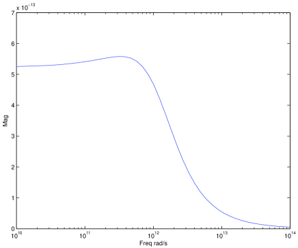
Figure 3: Magnitude Bode plot of $G_{\kappa_{1},\kappa_{2}}(s)$.

IV Conclusions

We have applied a previous result on the robust stability of nonlinear quantum systems to a quantum system arising from a Josephson junction coupled to an electromagnetic resonant cavity. This system involved a cosine function in the system Hamiltonian which was a suitable non-quadratic Hamiltonian leading to a quantum system with a sector bounded nonlinearity. For specific numerical values of the system parameters, it was shown that the robust stability result can be used to choose coupling parameters for the Josephson junction system in order to guarantee robust mean square stability.

References

• [1] M.ย Yanagisawa and H.ย Kimura, โ€œTransfer function approach to quantum control-part I: Dynamics of quantum feedback systems,โ€ IEEE Transactions on Automatic Control, vol.ย 48, no.ย 12, pp. 2107โ€“2120, 2003.
• [2] โ€”โ€”, โ€œTransfer function approach to quantum control-part II: Control concepts and applications,โ€ IEEE Transactions on Automatic Control, vol.ย 48, no.ย 12, pp. 2121โ€“2132, 2003.
• [3] N.ย Yamamoto, โ€œRobust observer for uncertain linear quantum systems,โ€ Phys. Rev. A, vol.ย 74, pp. 032โ€‰107โ€“1 โ€“ 032โ€‰107โ€“10, 2006.
• [4] M.ย R. James, H.ย I. Nurdin, and I.ย R. Petersen, โ€œHโˆžsuperscript๐ป{H}^{\infty} control of linear quantum stochastic systems,โ€ IEEE Transactions on Automatic Control, vol.ย 53, no.ย 8, pp. 1787โ€“1803, 2008.
• [5] H.ย I. Nurdin, M.ย R. James, and I.ย R. Petersen, โ€œCoherent quantum LQG control,โ€ Automatica, vol.ย 45, no.ย 8, pp. 1837โ€“1846, 2009.
• [6] J.ย Gough, R.ย Gohm, and M.ย Yanagisawa, โ€œLinear quantum feedback networks,โ€ Physical Review A, vol.ย 78, p. 062104, 2008.
• [7] A.ย I. Maalouf and I.ย R. Petersen, โ€œBounded real properties for a class of linear complex quantum systems,โ€ IEEE Transactions on Automatic Control, vol.ย 56, no.ย 4, pp. 786 โ€“ 801, 2011.
• [8] โ€”โ€”, โ€œCoherent ${H}^{\infty}$ control for a class of linear complex quantum systems,โ€ IEEE Transactions on Automatic Control, vol.ย 56, no.ย 2, pp. 309โ€“319, 2011.
• [9] N.ย Yamamoto, H.ย I. Nurdin, M.ย R. James, and I.ย R. Petersen, โ€œAvoiding entanglement sudden-death via feedback control in a quantum network,โ€ Physical Review A, vol.ย 78, no.ย 4, p. 042339, 2008.
• [10] J.ย Gough and M.ย R. James, โ€œThe series product and its application to quantum feedforward and feedback networks,โ€ IEEE Transactions on Automatic Control, vol.ย 54, no.ย 11, pp. 2530โ€“2544, 2009.
• [11] J.ย E. Gough, M.ย R. James, and H.ย I. Nurdin, โ€œSqueezing components in linear quantum feedback networks,โ€ Physical Review A, vol.ย 81, p. 023804, 2010.
• [12] H.ย M. Wiseman and G.ย J. Milburn, Quantum Measurement and Control.ย ย ย Cambridge University Press, 2010.
• [13] I.ย R. Petersen, โ€œQuantum linear systems theory,โ€ in Proceedings of the 19th International Symposium on Mathematical Theory of Networks and Systems, Budapest, Hungary, July 2010.
• [14] M.ย James and J.ย Gough, โ€œQuantum dissipative systems and feedback control design by interconnection,โ€ IEEE Transactions on Automatic Control, vol.ย 55, no.ย 8, pp. 1806 โ€“1821, August 2010.
• [15] I.ย R. Petersen, V.ย Ugrinovskii, and M.ย R. James, โ€œRobust stability of uncertain quantum systems,โ€ in Proceedings of the 2012 American Control Conference, Montreal, Canada, June 2012.
• [16] W.ย Al-Saidi and D.ย Stroud, โ€œEigenstates of a small Josephson junction coupled to a resonant cavity,โ€ Physical Review B, vol.ย 65, p. 014512, 2001.