Linear and quadratic temperature dependence
of electronic specific heat for cuprates

Abstract

We model cuprate superconductors as an infinite layered lattice structure which contains a fluid of paired and unpaired fermions. Paired fermions, which are the superconducting carriers, are considered as noninteracting zero spin bosons with a linear energy-momentum dispersion relation, which coexist with the unpaired fermions in a series of almost two dimensional slabs stacked in their perpendicular direction. The inter-slab penetrable planes are simulated by a Dirac comb potential in the direction in which the slabs are stacked, while paired and unpaired electrons (or holes) are free to move parallel to the planes. Paired fermions condense at a BEC critical temperature at which a jump in their specific heat is exhibited, whose values are assumed equal to the superconducting critical temperature and the specific heat jump experimentally reported for YBaCuO_7-x to fix our model parameters: the plane impenetrability and the fraction of superconducting charge carrier. We straightforwardly obtain, near and under the superconducting temperature $T_{c}$, the linear ($\gamma_{e}T$) and the quadratic ($\alpha T^{2}$) electronic specific heat terms, with $\gamma_{e}$ and $\alpha$ of the order of the latest experimental values reported. After calculating the lattice specific heat (phonons) $C_{l}$ from the phonon spectrum data obtained from inelastic neutron scattering experiments, and added to the electronic (paired plus unpaired) $C_{e}$ component, we qualitatively reproduce the total specific heat below $T_{c}$, whose curve lies close to the experimental one, reproducing its exact value at $T_{c}$.

I Introduction

From the discovery of cuprate High Temperature Superconductors in 1986 (HTSC) Bednorz many efforts have been made to explain the nature of their microscopic behavior as they are not completely described by the BCS theory BCS . The HTSC cuprates are perhaps the most studied both experimentally and theoretically until FeAs showed up. Their main characteristics can be summarized as follows: a small coherence length, usually of one or two nanometers; they have preferably either tetragonal or orthorombic crystallographic structures; and the Cooper pairs, responsible for the superconductivity, move in the copper oxide planes which resemble a quasi-2D layered system. They also modify their structure Poole2007 and their critical temperature $T_{c}$ by changing the oxygen concentration, being this feature responsible for achieving or not superconductivity for a same compound with different oxygen concentrations.

Particularly, the specific heat of the YBa₂Cu₃O_7-x cuprates, where $x$ represents the oxygen dopage made with holes, has been widely studied and we want to point out four key characteristics which have been observed. First of all, even though it is not easy to observe, below $T_{c}$ there is a linear term $\gamma_{e}T$ in the electronic specific heat, with $\gamma_{e}$ the electronic specific heat parameter or Sommerfeld constant - sometimes referred to as $\gamma(0)$-, whose latest reported values are between $2-3$ mJ/mol K² WangPhysRevB2001 . This term is currently believed to come from the normal state electronic specific heat (see Ref. Fisher2007 and references therein). In the second place, also at temperatures below $T_{c}$, there is an $\alpha T^{2}$ term in zero magnetic field Wright99 ; Moler97 ; WangPhysRevB2001 (initially denied in some reports Wright96 ), which changes to a $H^{1/2}T$ component in the presence of an external magnetic field $H$, and is attributable to the superconducting part of the electronic specific heat. The reported values for this constant are of the order of tenths of mJ/mol K³ WangPhysRevB2001 , but as it happens for the linear term coefficient, the obtained values depend strongly on the conditions of each experiment and on the theoretical method each author uses to subtract the other specific heat components. In the third place we have a “jump” (at zero magnetic field) in the specific heat at $T_{c}$ Junod97 indicating a second order phase transition (which becomes a “peak” at finite magnetic field) and is widely believed to be the result of the influence of the superconducting electronic specific heat $C_{es}$. Finally, the total specific heat divided by temperature $C/T$ shows an “upturn” (or “fishtail”) for temperatures under 5 K, which several authors Fisher2007 claim has an intrinsic magnetic origin, present even at zero external magnetic field. This latter low temperature feature has been modeled as a contribution of five terms: normal electronic $C_{en}$, superconducting electronic $C_{es}$, lattice $C_{l}$, magnetic and hyperfine specific heats Fisher88 ; Fisher2007 , even though the dynamic mechanism beneath them is not completely known.

Contrary to what one might think, to our knowledge, the lattice specific heat $C_{l}$ of a cuprate is not fully described by standard theories. This specific heat is generally considered as a contribution that doesn’t change with the superconductivity onset and it has been observed to behave as a $T^{3}$ term below 5 K WangPhysRevB2001 . For the lattice specific heat a number of proposals have been made, such as: use of the Born-von Kármán formalism Kittel applied to the multiatomic anisotropic lattice; fits of Debye and/or Einstein models Indios ; Inderhees87 ; Junod89 ; the use of different polynomials or power series on a number of different variables Inderhees92 ; Phillips1992 ; Gordon89 ; Bessergenev ; adaptation of models that have given successful results in other elements (such as ⁴He) Roulin96 ; Roulin98 ; Junod99 ; the use of the lower Landau level (LLL) formalism Junod99 , to mention a few.

On the other hand, experimentalists have been using indirect methods for obtaining the electronic specific heat $C_{e}$ - although a distinction between the normal and the superconducting part is sometimes not recognized - usually by separating the lattice specific heat from the total. For example, Loram et al. Loram93 , construct the lattice specific heat using a non-superconducting reference sample, using either a small variation on the oxygen content or introducing another element; or Meingast et al. Meingast09 , who construct their phonon density of states using a local-density approximation; or Bessergenev et al. Bessergenev , who develop a power series in terms of characteristic temperatures which depend on phononic moments; or using an estimated phonon spectrum based on known lattice vibration frequencies and inserting it in a set of Einstein functions with characteristic temperatures Shaviv . In all these studies, the authors subtract the “lattice” specific heat obtained from the total experimental specific heat of the cuprate, and what is left is reported as the “electronic specific heat”, which appears as a small contribution, restricted mainly to the height of the jump of only a few percent ($1-2\%$), and unwillingly transferring the intrinsic uncertainties of their method to $C_{e}$. Based on our results, we propose that this manipulation should be reconsidered, since in this work we show that the electronic specific heat (normal and superconducting) contributes with a ($30-40$)$\%$ of the total.

For conventional superconductors $\gamma_{e}$ can be obtained from the linear term of the electronic specific heat in the normal state $C_{en}$, while the superconducting component $C_{es}$ has an exponential behavior at very low temperatures predicted by BCS. For HTSC this term has been confirmed to exist even in the superconducting state, however, it is very difficult to separate it from the other components due to thermal fluctuations and to the need of very high external magnetic fields to suppress the characteristic upturn WangPhysRevB2001 ; Fisher2007 . The importance of determining the value of $\gamma_{e}$ lies on its direct relation to the electronic density of states and on the belief that it gives information about the interaction electron-phonon Fisher2007 . In addition, there are models, such as Anderson’s Resonating Valence Bond (RVB) Anderson , that predict a linear term in the specific heat, but until now, the controversy over whether $\gamma_{e}$ comes from a residual zero-field term, from the superconducting electronic specific heat Fisher2007 or from normal electrons that didn’t participate in the superconducting state (see, for example, UherCardwell p.85) goes on. In this work we adopt this point of view and consider the linear part of the electronic specific heat, $\gamma_{e}T$, is a result of unpaired electrons inside a layered structure, as we will show.

Even though conventional superconductors do not exhibit an $\alpha T^{2}$ electronic specific heat term, it has experimentally been confirmed that HTSC do WangPhysRevB2001 . Most of the reported values for this constant were obtained by first fixing $\gamma_{e}$ and then fitting curves with other parameters Wright99 ; Moler97 , while others Revaz98 ; WangPhysRevB2001 set an arrange of different external magnetic fields to cancel the interfering components. In the model presented in this paper, such a quadratic in temperature term in the electronic specific heat comes from paired electrons (superconducting state), and values of $\alpha$ are of the order of some ones reported experimentally Bessergenev .

At zero external magnetic field, the “jump” $\Delta C$ in the specific heat at the transition temperature has also been reported with a great variety of values depending on each experiment. Currently, this feature is attributed to the electronic specific heat, its magnitude is of $\Delta C\approx 5$ J/mol K according to several authors Gordon89 ; Inderhees92 ; Shaviv ; Junod89 , and it has also been shown that for the same sample its jump diminishes as the magnitude of an external magnetic field is increased Junod97 . As experiments have become more accurate, the shape of the jump has become sharper WangPhysRevB2001 . However, a roundness of the curves at the jump with positive curvature is usually justified by the finiteness of the samples and by the presence of thermal fluctuations, which are important in HTSC Inderhees91 .

In the framework of the most basic Boson-Fermion model Friedberg1989a ; Friedberg1989b ; Casas2001 ; Adhikari2000 of superconductivity, we assume Cooper pairs are composite-spin-zero-bosons with either zero or nonzero moments of center of mass, coexisting with a fermion fluid formed by the unpaired electrons. These Cooper pairs are pre-formed at some temperature $T^{\ast}>T_{c}$ and can undergo a Bose-Einstein condensation (BEC) as temperature is lowered Casas2001 ; Eagles . We are aware that the number of preformed pairs increases as the temperature is lowered until $T_{c}$, where its density is large enough to achieve coherence, independently of the mechanism by which the pairs are formed. Below $T_{c}$ we assume that the number of pairs remains constant.

On the other hand, in order to include the effect of the layered structure of cuprates in the Boson-Fermion model, we previously calculated the BEC critical temperature and the thermodynamic properties for a system of non-interacting bosons immersed in a periodic multilayer array which represents the confinement agent PatyJLTP2010 ; Paty2 . The multilayer array is simulated by an external Kronig-Penney (KP) potential at the delta limit case along the perpendicular direction to the CuO₂ planes, while the particles are allowed to move freely in the parallel directions with an energy-momentum dispersion relation where the linear term predominates, as has been shown in [Adhikari2000, ].

Our system model begins with $N$ electrons of mass $m_{e}$ interacting via a BCS type potential. There is a subgroup of electrons able to form pairs (Cooper pairs), since they are within a shell of width $2\hbar\omega_{D}$ around the Fermi energy $E_{F}$, where $\hbar\omega_{D}$ is the Debye energy, coexisting with a non-pairable group of electrons formed by those under and above the pairing shell, and are not eligible for pairing. From the first group, which we call the pairable electrons, we consider that only a fraction of them are paired, these are equal to a smaller fraction $fN/2$ which participate in the superconductivity; our assumption is based on the analysis of Uemura’s plot (Fig. 2 of Ref Uemura2006 ) that shows that critical temperatures for cuprates are in the empirical range of $T_{c}\approx(0.01-0.06)T_{F}$ AdhikariPhysC2000 . With all the stated above in mind, the $N$ electrons are grouped in three major components: paired electrons (boson gas) formed by a fraction $f$ of half the total $N$ electrons (inside the pairing shell); a fermion gas formed by the pairable but unpaired electrons (also inside the pairing shell); and the unpairable electrons (outside the pairing shell); plus a phonon gas due to the lattice. In Sec. II.1 we obtain the grand potential from where it is possible to derive all the thermodynamic properties. This model depends on three physical properties: the separation between planes $a$; the impenetrability $P_{0}$ of the planes, which is responsible for the anisotropy observed in cuprates; and the density of superconducting carriers $fn/2$, with $n$ the fermionic number density. In section II.2 we fix $a$ with the experimental values reported and calculate the critical temperature of the boson gas made of Cooper pairs as a function of $P_{0}$ and $f$.

In section III.1 we obtain the superconducting electronic specific heat for the Cooper pairs fixing the unknown parameters $P_{0}$ and $f$ with the experimental $T_{cexp}$ and the magnitude of the “jump” in the electronic specific heat at $T_{c}$. As a consequence $C_{es}$ shows the observed $T^{2}$ behavior. Meanwhile, in section III.2 we derive the expressions for the normal electronic specific heat of the total unpaired $(1-f)N$ electrons (fermions) in a periodic layered structure, which shows the expected linear dependence on $T$. In Sec. III.3 we add the two contributions and show that the total electronic specific heat at and under $T_{c}$ has the same behavior obtained by experiments. The electronic specific constants we obtain are $\gamma_{e}$ = 5.2 mJ/mol K² and $\alpha$ = 4.3 mJ/mol K³, compared to 2.19 and 0.21 reported in WangPhysRevB2001 , and to 25.1 and 3.4 reported in Bessergenev . In addition, since the lattice specific heat represents the main contribution of the total specific heat, in section IV we calculate the specific heat for the phonons using two different approaches: Debye model and phonon density of states from inelastic neutron scattering (INS) experiments Renker88 . In section V, we sum these three specific heat contributions and compare the result with experiments. We find an excellent qualitative agreement with the experimental $C$, where the contribution of the electronic specific heat is a significant part of the total. Finally, in Sec. VI we present our conclusions.

II Cooper pairs in a layered structure

We begin by taking a group of pairable electrons immersed in a periodic layered array along the $z$ direction and free to move in the other two directions with a linear dispersion relation. The wave vector for the center of mass of the pair (CMM) is given by $\mathbf{K}=(K_{x},K_{y},K_{z})\equiv\mathbf{k_{1}}+\mathbf{k_{2}}$, while $\mathbf{k}\equiv 1/2(\mathbf{k_{1}}-\mathbf{k_{2}})$ is the relative momentum, where $\mathbf{k_{1}}$ and $\mathbf{k_{2}}$ are the wave vectors of each electron of the pair. The solution for the Schrödinger equation for the pairs may be separated in the $x-y$ and $z$ directions, so the energy for each particle is $\varepsilon_{K}=\varepsilon_{K_{x,y}}+\varepsilon_{K_{z}}$. Here the total pair energy in the plane is $\varepsilon_{K_{x,y}}\equiv 2E_{F}-\Delta_{K}$, with $\Delta_{K}$ the binding energy of the pair for any temperature and any center of mass momentum. It has been shown that when $\mathbf{K}$ is non zero, but small, one can expand the binding energy from the Cooper equation in a series of powers Adhikari2000 , so the total energy in the plane is

$$\varepsilon_{K_{x,y}}=\mathsf{e}_{0}+C_{1}(K_{x}^{2}+K_{y}^{2})^{1/2}+O(K^{2}),$$ (1)

where $\mathsf{e}_{0}\equiv 2E_{F}-\Delta_{0}$ is a constant, $C_{1}=(2/\pi)\hbar\mathsf{v}_{F2D}$ is the linear term coefficient in 2D, $\mathsf{v}_{F2D}$ is the corresponding Fermi velocity, $\Delta_{0}=2\hbar\omega_{D}\exp(-1/\lambda)$ is the energy gap for $\mathbf{K}=0$ and weak coupling (corresponding to the BCS theory), and $\lambda\equiv g(E_{F})V$ the dimensionless coupling constant in terms of the electronic density of states at the Fermi sea $g(E_{F})$ and the non-local interaction $V$.

Along the $z$-direction we use the Kronig-Penney KP potential, where the energies are implicitly obtained, as a function of $a$, from the transcendental equation

$$P_{0}(a/\lambda_{0})\sin(\alpha_{K_{z}}a)/\alpha_{K_{z}}a+\cos(\alpha_{K_{z}}a)=\cos(K_{z}a),$$ (2)

with $\alpha_{K_{z}}^{2}\equiv 2m\varepsilon_{K_{z}}/\hbar^{2}$, $m=2m_{e}$ the mass of the composite-boson, and we have defined the dimensionless plane impenetrability $P_{0}\equiv P\lambda_{0}/a=m\Lambda\lambda_{0}/\hbar^{2}$. The constant $\lambda_{0}\equiv h/\sqrt{2\pi mk_{B}T_{0}}$ is the de Broglie thermal wavelength of an ideal boson gas in an infinite box at the BEC critical temperature $T_{0}=2\pi\hbar^{2}n_{B}^{2/3}/mk_{B}\zeta(3/2)^{2/3}\simeq 3.31\hbar^{2}n_{B}^{2/3}/mk_{B}$, with $n_{B}\equiv N/(2L^{3})$ the boson number density and $\Lambda$ is the strength of the KP delta potentials $\sum_{n_{z}=-\infty}^{\infty}\Lambda\delta(z-n_{z}a)$.

Note that when $P_{0}\rightarrow 0$ the energy goes to the free-particle energy $\varepsilon_{K_{z}}\rightarrow\hbar^{2}K_{z}^{2}/2m$ in the $z$ direction. Also, when we have small energies, $\varepsilon_{K_{z}}<$ $\hbar^{2}\pi^{2}/2ma^{2}$, we get the approximation

$$\varepsilon_{K_{z}}\cong\varepsilon_{0}+\frac{\hbar^{2}}{Ma^{2}}(1-\cos K_{z}a),$$ (3)

where $\varepsilon_{0}\equiv\hbar^{2}{\alpha_{0}}^{2}/2m$ is the solution of Ec. (2) when $K_{z}\rightarrow 0$ and $M$ is an effective mass Paty2 ; PatyJLTP2010 . Ec. (3) is the most commonly used expression for quasi-bidimensional models of superconductors (see for example WK ), but it is a very limited model, since it involves calculations only over the first energy band and with $\varepsilon_{0}=0$ the ground state energy. In this work we use the exact solution of the Eq. (2).

II.1 Grand potential

To calculate the thermodynamic properties we begin with the grand potential $\Omega(T,L^{3},\mu)$, which for a boson gas with $N_{B}$ particles contained in a volume $V\equiv L^{3}$ Path is

$$\Omega(T,L^{3},\mu)=U-TS-\mu N_{B}=\Omega_{0}+k_{B}T\sum_{\mathbf{K}{\neq 0}}\ln\bigl{\{}1-$$

$$\exp[-\beta(\mathsf{e}_{0}+C_{1}(K_{x}^{2}+K_{y}^{2})^{1/2}+\varepsilon_{K_{z}}-\mu)]\bigr{\}},$$ (4)

where $U$ is the internal energy, $S$ the entropy, $\mu$ the chemical potential, $\beta\equiv 1/k_{B}T$, and the first term in the rhs corresponds to the $\mathbf{K}={0}$ ground state energy contribution $\Omega_{0}$ = $k_{B}T\ln\{1-\exp[-\beta(\varepsilon_{0}+\mathsf{e}_{0}-\mu)]\}$.

Using that $\ln(1-x)=-\sum_{l=1}^{\infty}x^{l}/l$ in Ec. (4), and after some algebra we have

$$\Omega(T,L^{3},\mu)=\Omega_{0}-k_{B}T\sum_{l=1}^{\infty}\sum_{\mathbf{K}{\neq 0}}\frac{\exp\bigl{\{}\beta(\mu-\mathsf{e}_{0})l\bigr{\}}}{l}$$

$$\times\exp\bigl{\{}-\beta(C_{1}(K_{x}^{2}+K_{y}^{2})^{1/2}+\varepsilon_{K_{z}})l\bigr{\}}.$$ (5)

By substituting sums by integrals in the thermodynamic limit, and doing the integrals over $x,y$ one gets

$$\Omega\left(T,L^{3},\mu\right)=k_{B}T\ln\bigl{\{}1-\exp[-\beta(\varepsilon_{0}+\mathsf{e}_{0}-\mu)\bigr{\}}-$$

$$\frac{1}{\beta^{3}}\frac{L^{3}}{\left(2\pi\right)^{2}}\frac{\Gamma(2)}{C_{1}^{2}}{\int_{-\infty}^{\infty}dK_{z}}\ \mathsf{g}_{3}\bigl{\{}\exp[-\beta(\varepsilon_{K_{z}}+\mathsf{e}_{0}-\mu)]\bigr{\}}.$$ (6)

where we have used the Bose functions $\mathsf{g}_{\sigma}(t)\equiv\sum_{l=1}^{\infty}(t)^{\mathit{l}}/\mathit{l}^{\sigma}$. From (6) we can find the thermodynamic properties for a monoatomic Bose gas PatyJLTP2010 ; Paty2 .

II.2 Critical temperature

To obtain the critical temperature of the boson gas we use the expression for the bosonic particle number, which we calculate summing the number of particles in each energy state, therefore

$$N_{B}=\frac{1}{\exp\bigl{\{}\beta(\varepsilon_{0}+\mathsf{e}_{0}-\mu)\bigr{\}}-1}+$$

$$\frac{L^{3}}{\left(2\pi\right)^{2}}\frac{\Gamma(2)}{C_{1}^{2}}\frac{1}{\beta^{2}}{\int_{-\infty}^{\infty}dK_{z}}\mathsf{g}_{2}\bigl{\{}\exp[-\beta(\varepsilon_{K_{z}}+\mathsf{e}_{0}-\mu)]\bigr{\}},$$ (7)

where the first term of the rhs corresponds to the number of particles in the condensate $N_{0}(T)$ and the second term to the ones in the excited state $N_{e}(T)$.

We must notice here that from the relation for the Fermi energy Path , $E_{F}={\hbar^{2}}(3\pi^{2})^{2/3}n_{s}^{2/3}/2m^{\ast}$, with $E_{F}$ the Fermi energy which corresponds to a Fermi temperature of $T_{F}$ = 2290 K for the cuprate and $m^{\ast}=2m_{e}$ the effective mass of the carriers, one gets that the density number of carriers is $n_{s}=1.128\times 10^{27}/$m³. On the other hand, from the relation $T_{0}/T_{F}=0.218$ Sevilla one gets $T_{0}=499.2$ K, when all the fermions in the cuprate are paired. Using this boson gas temperature and from the definition of $T_{0}$, one gets $n_{B}=1.994\times 10^{26}/$m³, the boson density number of an ideal gas, whose value is an order of magnitude smaller than $n_{s}$. However, as we previously stated, analyzing the data in Fig. 2 of Ref Uemura2006 , and localizing the diagonal lines labeled as $T=T_{F}$ and $T=T_{0}$ (identified as $T_{B}$), one would expect that the actual quantity of superconducting carriers $n_{b}$ for the cuprate materials would be at least two orders of magnitude smaller than the $n_{s}$ given above. Therefore, we assume that only a fraction $f$ of the maximum possible value $n_{B}$ is participating in the boson gas responsible for the superconductivity, so $n_{b}=fn_{B}$, and we expect this factor to lie in the interval $f\in[0.01,0.14]$, according to what is explained in Ref. AdhikariPhysC2000 .

The BEC temperature of this boson gas in the thermodynamic limit is

$$T_{0f}=\frac{2\pi\hbar^{2}n_{b}^{2/3}}{mk_{B}\zeta(3/2)^{2/3}}=T_{0}f^{2/3}.$$ (8)

For $f=1$ we recover the case where all pairable fermions participate in the boson gas. The corresponding thermal wavelenght is $\lambda_{0f}=h/\sqrt{2\pi mk_{B}T_{0f}}=\lambda_{0}/f^{1/3}$. The quotient of the fraction of an ideal gas BEC temperature over the Fermi temperature of the whole is Sevilla

$$\frac{T_{0f}}{T_{F}}=\frac{2\pi f^{2/3}}{(6\pi^{2})^{2/3}\zeta(3/2)^{2/3}}=(0.218)f^{2/3}.$$ (9)

Now we use the relation for the 3D Fermi energy $E_{F3{\text{D}}}=[(3\pi^{2})^{2/3}/2\pi]E_{F2{\text{D}}}$ for a 3D system in terms of the Fermi energy for a 2D system $E_{F2{\text{D}}}=\frac{1}{2}m_{e}\mathsf{v}_{F2D}^{2}$. The constant $C_{1}^{2}=(4/\pi^{2})\hbar^{2}\mathsf{v}_{F2D}^{2}=[64/\pi(3\pi^{2})^{2/3}]\gamma a^{2}E_{F3D}k_{B}T_{0}$, where $\gamma\equiv\hbar^{2}/2ma^{2}k_{B}T_{0}$ is a dimensionless constant. Introducing $f$ in (7), dividing by $N$ and taking $T=T_{c}$, so the chemical potential $\mu_{0}=\varepsilon_{0}+\mathsf{e}_{0}$ and $N_{0}(T_{c})\simeq 0$, we have

$$1=\frac{2}{f}\frac{\Gamma(2)3\pi(3\pi^{2})^{2/3}}{128}\left(\frac{0.436\gamma T_{0}}{T_{F}}\right)^{1/2}\frac{1}{(k_{B}T_{F}\beta_{c})^{2}}$$

$$\times\int_{0}^{\infty}adK_{z}\mathsf{g}_{2}\bigl{\{}\exp[-k_{B}T_{F}\beta_{c}\gamma(T_{0}/T_{F})(\bar{\varepsilon}_{K_{z}}-\bar{\varepsilon}_{0})]\bigr{\}}.$$ (10)

where $\bar{\varepsilon}_{K_{z}}\equiv\varepsilon_{K_{z}}/(\hbar^{2}/2ma^{2})$, and $\bar{\varepsilon}_{0}\equiv\varepsilon_{0}/(\hbar^{2}/2ma^{2})$ are dimensionless energies obtained numerically from (2) for each band.

We split the infinite integral in (10) as a sum of integrals over the allowed energy bands, fold every band over the first half Brillouin zone (from $0$ to $\pi$) and cut the sum at the $J$-th band once convergence has been achieved. Finally, using the numerical value $\Gamma(2)3\pi(3\pi^{2})^{2/3}(0.436T_{0}/T_{F})^{1/2}/(128)=0.46532$ we arrive to

$$1=\frac{2}{f}0.46532\gamma^{1/2}\frac{1}{(k_{B}T_{F}\beta_{c})^{2}}$$

$$\times\sum_{j=1}^{J}\int_{0}^{\pi}adK_{z}\mathsf{g}_{2}\bigl{\{}\exp[-k_{B}T_{F}\beta_{c}\gamma(T_{0}/T_{F})(\bar{\varepsilon}_{K_{z}}-\bar{\varepsilon}_{0})]\bigr{\}},$$ (11)

which must be solved numerically. From now on we will be using this allowed-band-splitting method for evaluating the infinite integrals.

Figure 1: Critical temperature as a function of $P_{0}$ for different values of $f$. Dashed line is the experimental $T_{c}=92.2$ K for the cuprate.

The experimental parameters for the cuprate YBa₂Cu₃O_6.92 that we use are: the critical temperature $T_{cexp}$ = 92.2 K Bessergenev ; the Fermi temperature $T_{F}=2290$ K Poole95 ; $\Delta_{0}=20$ meV WangPhysRevB2001 ; the parameter $a=5.85$ Å corresponding to $a=c/2$ ($c=11.69$ Å the crystallographic constant), the distance between a copper oxide plane located at the extreme of the unitary cell and the Ytrium atom at the center. This is based on the knowledge that superconductivity occurs in the close vicinity parallel to the CuO₂ planes, which are two per unit cell. We can also calculate the thermal wavelength $\lambda_{0}=23.575$ Å , and the parameters $a/\lambda_{0}=0.246$ and $\gamma=1.317$. Finally, we obtain the magnitud of the jump $\Delta C/T_{c}$ $\simeq$ 20 mJ/mol K² from the data published by Bessergenev . It is well known that in cuprates there is an optimum oxygen dopage for which $T_{c}$ is higher Roulin98 , but we choose the dopage for which we find more accurate experimental data.

In Fig. 1 we show the critical temperature as a function of the parameter $P_{0}$ for five values of $f$. The dashed line represents the experimental critical temperature for YBa₂Cu₃O_6.92. As we can see from this figure, there is only a narrow interval of values of $f\in[0.001,0.02]$, that suits the experimental condition $T_{cexp}$ = 92.2 K, consistent with what we expected, which in turn determines a set of values of $P_{0}$. This means that only a small percentage of the initially pairable fermions form pairs, as we argued above. To determine exactly both values, we choose a second feature of the electronic specific heat: the magnitude of the jump.

II.3 Internal Energy

We can derive the internal energy of the pair’s gas as

$$U(T,V)=\frac{(\varepsilon_{0}+\mathsf{e}_{0})}{\exp\bigl{\{}\beta(\varepsilon_{0}+\mathsf{e}_{0}-\mu)\bigr{\}}-1}+\frac{L^{3}}{\left(2\pi\right)^{2}}\frac{\Gamma(2)}{C_{1}^{2}}\frac{1}{\beta^{2}}\times$$

$${\int_{-\infty}^{\infty}dK_{z}}(\mathsf{e}_{0}+\varepsilon_{K_{z}})\mathsf{g}_{2}\bigl{\{}\exp[-\beta(\varepsilon_{K_{z}}+\mathsf{e}_{0}-\mu)]\bigr{\}}$$

$$+2\frac{L^{3}}{\left(2\pi\right)^{2}}\frac{\Gamma(2)}{C_{1}^{2}}\frac{2}{\beta^{3}}{\int_{-\infty}^{\infty}dK_{z}}\mathsf{g}_{3}\bigl{\{}\exp[-\beta(\varepsilon_{K_{z}}+\mathsf{e}_{0}-\mu)]\bigr{\}},$$ (12)

where the first term corresponds to the particles in the ground state, $(\varepsilon_{0}+\mathsf{e}_{0})N_{0}$. From the previous equation we subtract the ground state energy times the total number of pairs given by the number equation (7), then multiply the result by $f$ and divide it by $N_{B}k_{B}T$, so we have

$$\frac{(U-(\varepsilon_{0}+\mathsf{e}_{0})N_{B})}{N_{B}k_{B}T}=\frac{2}{f}0.46532\left(\frac{2T_{0}}{T_{F}}\right)\gamma^{3/2}\times$$

$$\frac{1}{k_{B}T_{F}\beta}{\int_{-\infty}^{\infty}adK_{z}}(\bar{\varepsilon}_{K_{z}}-\bar{\varepsilon}_{0})\mathsf{g}_{2}\bigl{\{}\exp[-k_{B}T_{F}\beta\gamma(T_{0}/T_{F})\times$$

$$(\bar{\varepsilon}_{K_{z}}+\bar{\mathsf{e}}_{0}-\bar{\mu})]\bigr{\}}+\frac{4}{f}0.46532\gamma^{1/2}\frac{1}{{(k_{B}T_{F}\beta)}^{2}}$$

$$\times{\int_{-\infty}^{\infty}}adK_{z}\mathsf{g}_{3}\{\exp[-k_{B}T_{F}\beta\gamma(T_{0}/T_{F})(\bar{\varepsilon}_{K_{z}}+\bar{\mathsf{e}}_{0}-\bar{\mu})]\}.$$ (13)

In order to compute the internal energy and the specific heat it is necessary to get numerically the chemical potential and its derivative with respect to $T$. From the number equation (7) and by making the considerations that $\mu=\mu_{0}$ if $T<T_{c}$, and $N_{0}/N_{b}\sim 0$ for $T>T_{c}$, $\mu$ is obtained from

$$1=\frac{2}{f}0.46532\gamma^{1/2}\frac{1}{(k_{B}T_{F}\beta)^{2}}\int_{-\infty}^{\infty}adK_{z}\times$$

$$\mathsf{g}_{2}\bigl{\{}\exp[-(k_{B}T_{F}\beta)\gamma(T_{0}/T_{F})(\bar{\varepsilon}_{k_{z}}+\bar{\mathsf{e}}_{0}-\bar{\mu})]\bigr{\}},$$ (14)

and its derivative is given by

$$T\frac{d\bar{\mu}}{dT}=\biggl{[}2k_{B}T_{F}\beta-\frac{2}{f}0.46532\gamma^{3/2}\left(\frac{T_{0}}{T_{F}}\right){\int_{-\infty}^{\infty}}adK_{z}\times$$

$$\ln\{1-\exp[-k_{B}T_{F}\beta\gamma(T_{0}/T_{F})(\bar{\varepsilon}_{K_{z}}-\bar{\mu}+\bar{\mathsf{e}}_{0})]\}\times$$

$$(\bar{\varepsilon}_{K_{z}}-\bar{\mu}+\bar{\mathsf{e}}_{0})\biggr{]}/\biggl{[}\frac{2}{f}0.46532\gamma^{3/2}\left(\frac{2T_{0}}{T_{F}}\right){\int_{-\infty}^{\infty}}adK_{z}\times$$

$$\ln\{1-\exp[-k_{B}T_{F}\beta\gamma(T_{0}/T_{F})(\bar{\varepsilon}_{K_{z}}-\bar{\mu}+\bar{\mathsf{e}}_{0})]\}\biggr{]}.$$ (15)

III Electronic specific heat

We consider that the electronic specific heat $C_{e}$ of the cuprate is formed by the specific heat of the gas of Cooper-pairs, plus the specific heat of the gas of all the remaining electrons that didn’t form pairs.

Like most authors do, we assume that the electronic specific heat is responsible for the jump, which in turn provides the information about the phase transition.

In this model approach, we also consider that the specific heat at constant volume $C_{V}$ is the same as the specific heat at constant pressure $C_{p}$ at least from $T=0$ to $200$ K, as has been established for cuprates by several authors Meingast91 ; Nagel ; Jorgensen ; Meingast09 . So from now on we will drop any subscript on this matter.

III.1 Superconducting electronic specific heat

We are able to get the superconducting electronic specific heat $C_{es}$ by introducing the internal energy (12) in $C_{es}=\left[{\frac{\partial}{\partial T}}U(T,L^{3})\right]_{N,L^{3}}$, and taking the fraction $f$

$$\frac{C_{es}}{N_{b}k_{B}}=\frac{2}{f}0.46532\left(\frac{2T_{0}}{T_{F}}\right)\gamma^{3/2}\frac{1}{(k_{B}T_{F}\beta)}$$

$$\times\int_{-\infty}^{\infty}adK_{z}\ \mathsf{g}_{2}\{\exp[-k_{B}T_{F}\beta\gamma(T_{0}/T_{F})(\bar{\varepsilon}_{K_{z}}-\bar{\mathsf{e}}_{0}-\bar{\mu})]\}$$

$$\times[2\bar{\varepsilon}_{K_{z}}-\bar{\varepsilon}_{0}+\bar{\mathsf{e}}_{0}-\bar{\mu}+T\frac{d\bar{\mu}}{dT}]$$

$$-\frac{1}{2f}0.46532\left(\frac{2T_{0}}{T_{F}}\right)^{2}\gamma^{5/2}\int_{-\infty}^{\infty}adK_{z}(\bar{\varepsilon}_{K_{z}}-\bar{\varepsilon}_{0})$$

$$\times\ln\{1-\exp[-k_{B}T_{F}\beta\gamma(T_{0}/T_{F})(\bar{\varepsilon}_{K_{z}}+\bar{\mathsf{e}}_{0}-\bar{\mu})]\}$$

$$\times[\bar{\varepsilon}_{K_{z}}+\bar{\mathsf{e}}_{0}-\bar{\mu}+T\frac{d\bar{\mu}}{dT}]+\frac{12}{f}0.46532\gamma^{1/2}\frac{1}{{(k_{B}T_{F}\beta)}^{2}}$$

$$\times\int_{-\infty}^{\infty}adK_{z}\mathsf{g}_{3}\{\exp[-k_{B}T_{F}\beta\gamma(T_{0}/T_{F})(\bar{\varepsilon}_{K_{z}}+\bar{\mathsf{e}}_{0}-\bar{\mu})]\}.$$ (16)

In Figs. 2 and 3 we present the superconducting electronic specific heat $C_{es}$ and $C_{es}/T$ as function of temperature for the gas of Cooper pairs. The height of the jump is reproduced by taking the values $f=0.018$ (which lies inside the interval [0.01, 0.14] obtained in Sec. II.2) and $P_{0}=3\times 10^{5}$ for the dimensionless parameters of our model.

Figure 2: Electronic specific heat as a function of $T$ for the Cooper pairs gas for YBa₂Cu₃O_6.92 using Ec. (16), using $f=0.018$ and $P_{0}=3\times 10^{5}$.

Figure 3: Electronic specific heat over temperature as a function of $T$ for the Cooper pairs gas for YBa₂Cu₃O_6.92.

The quadratic behavior of $C_{es}$ with temperature is clear from the curve presented in Fig 3, so we can extract the slope $\alpha=4.3$ mJ/mol K³. It is also important to point out that the percentage of paired electrons that participate in superconductivity is among 1 and 3$\%$, consistent with the report in WangPhysRevB2001 and in contrast to the 90 to 95$\%$ reported in Shaviv .

III.2 Normal electronic specific heat

We shall consider now the gas of fermions made of the electrons with mass $m_{e}$ in the spherical shell who didn’t pair to form Cooper pairs plus the unpairable electrons, constituting $(1-f)$ of the total $N$ electrons. The grand potential for an ideal fermi gas comes from Path

$$\Omega(T,L^{3},\mu_{fer})=-k_{B}T\sum_{\mathbf{k}{=0}}\ln\bigl{\{}1+\exp[-\beta(\varepsilon_{\mathbf{k}}-\mu_{fer})]\bigr{\}}.$$ (17)

where $\mu_{fer}$ is the chemical potential of the electron gas and $\varepsilon_{\mathbf{k}}=\hbar^{2}k_{x}^{2}/2m_{e}+\hbar^{2}k_{y}^{2}/2m_{e}+\varepsilon_{k_{z}}$ is the energy of each electron free in the $x-y$ directions and constrained by permeable planes in $z$ direction. As we did in the case of the boson gas, the $z$-component energy must come from the KP Eq. (2) taking the momentum of the electron $k_{z}$ and the corresponding impenetrability $P_{0F}$ = $P_{0}/2$. Replacing sums for integrals in the thermodynamic limit, and doing the integrals over $k_{x}$, $k_{y}$ we have

$$\Omega\left(T,L^{3},\mu_{fer}\right)=-2\frac{L^{3}}{\left(2\pi\right)^{2}}\frac{m_{e}}{\hbar^{2}}\frac{1}{\beta^{2}}$$

$$\times{\int_{-\infty}^{\infty}dk_{z}}\mathsf{f}_{2}(\exp[-\beta(\varepsilon_{k_{z}}-\mu_{fer})]),$$ (18)

where we have made use of the Fermi-Dirac functions $\mathsf{f}_{\sigma}(t)\equiv\sum_{l=1}^{\infty}(-1)^{l-1}t^{\mathit{l}}/\mathit{l}^{\sigma}$ Path .

In order to obtain the electronic specific heat for the fermions $C_{en}$ (sometimes referred to as $C_{lin}$ WangPhysRevB2001 ), first we deduce the internal energy of the fermi gas and then the specific heat, so doing the usual algebra we have

$$\frac{C_{en}}{N_{fer}k_{B}}=4\frac{1}{(1-f)}\frac{L^{3}}{N\left(2\pi\right)^{2}}\frac{m_{e}}{\hbar^{2}}\frac{1}{\beta}$$

$$\times{\int_{-\infty}^{\infty}dk_{z}}\mathsf{f}_{2}\{\exp[-\beta(\varepsilon_{k_{z}}-\mu_{fer})]\}+$$

$$2\frac{1}{(1-f)}\frac{L^{3}}{N\left(2\pi\right)^{2}}\frac{m_{e}}{\hbar^{2}}\int_{-\infty}^{\infty}dk_{z}\ln\{1+$$

$$\exp[-\beta(\varepsilon_{k_{z}}-\mu_{fer})]\}\{2\varepsilon_{k_{z}}-\mu_{fer}+T\frac{\partial\mu_{fer}}{\partial T}\}$$

$$+2\frac{1}{(1-f)}\frac{L^{3}}{N\left(2\pi\right)^{2}}\frac{m_{e}}{\hbar^{2}}\beta$$

$$\times{\int_{-\infty}^{\infty}dk_{z}}\frac{\varepsilon_{k_{z}}\{\varepsilon_{k_{z}}-\mu_{fer}+T\frac{\partial\mu_{fer}}{\partial T}\}}{\exp[\beta(\varepsilon_{k_{z}}-\mu_{fer})]+1},$$ (19)

where $N_{fer}$ is the number of non-paired fermions.

The chemical potential is calculated from the corresponding number equation as

$$1=\frac{1}{(1-f)}\frac{L^{3}}{N}\frac{2}{\left(2\pi\right)^{2}}\frac{m_{e}}{\hbar^{2}}\frac{1}{\beta}$$

$$\times{\int_{-\infty}^{\infty}dk_{z}}\ln\{1+\exp[-\beta(\varepsilon_{k_{z}}-\mu_{fer})]\}$$ (20)

from where $\mu_{fer}$ and its derivative are extracted using numerical methods.

In Fig. 4 we present the behavior of the normal electronic specific heat for the unpaired electrons taking the values of ($f,P_{0}$) obtained in the preceding section. Notice that $C_{en}$ is linear in $T$ until well above $T_{c}$, as expected, and its coeficient is $\gamma_{e}$ = 5.2 mJ/mol K².

Figure 4: Specific heat as a function of $T$ for the unpaired electrons, using $f=0.018$ and $P_{0F}=1.5\times 10^{5}$.

Clearly, there is a non-zero value for $\gamma_{e}$, as stated in some reports Liang for oxygen contents $x>0.6$, and it corresponds to the contribution of the unpaired electron, as suggested by Fisher, et al. in Fisher2007 .

The analysis of the thermodynamic properties of a gas of fermions in a layered structure will be made elsewhere.

III.3 Total electronic specific heat

The total electronic specific heat is the sum of the previous contributions: the Cooper pairs specific heat and the unpaired electrons specific heat, $C_{e}=C_{es}+C_{en}$. We find that the contribution of the normal state electronic specific heat is two orders of magnitude smaller than the superconducting counterpart (Cooper pairs), so in Fig. 5 we present the curve $C_{e}/T$ vs $T$, where the difference can be better appreciated, the dashed line being the normal electronic specific heat.

Figure 5: Specific heat over temperature $T$ for Cooper pairs plus unpaired electrons, using $f=0.018$ and $P_{0}=3\times 10^{5}$. The dashed line is the unpaired electrons contribution.

There are some considerations we would like to do at this point, based in our results. First, we do not reproduce the upturn for the $T<5$ K temperature region since the internal magnetic components and the influence of external magnetic fields are not considered, as expected. Second, we have the coexistence of the two gases at least for temperatures under $T_{c}$. Above $T_{c}$ paired fermions decouple in an unknown way, so we do not include the decoupling mechanism in our analysis. As a consequence of the coexistence of the two gases, there is a linear temperature component in the electronic specific heat, which comes from (at least) the normal part of the system, while the quadratic temperature term is a contribution of the bosonic superconducting counterpart. In some articles Indios it has been suggested that the linear component comes exclusively from the presence of holes, however, in this version of our model we can not discriminate between holes and electrons. And last, we are able to state that the contribution of the electronic specific heat to the total is around 30$\%$, and not only 1 - 2$\%$ as has been repeatedly suggested Loram93 ; Meingast09 .

IV Lattice specific heat

In this section we calculate the specific heat due to the lattice $C_{l}$, which represents the major contribution for any solid. To do so, we describe and use two different formalisms: a simple Debye model and a phenomenological procedure where we take the phonon spectrum from inelastic neutron scattering experiments, and compare both results. After this, we proceed to add the resulting curve to our previous electronic specific heat results.

The total internal energy of a crystal is in general obtained by taking the normal vibration mode number $G(\omega)d\omega$ which lie in an interval $\omega$, $\omega+d\omega$ with a frecuency $\omega$, where $G(\omega)$ is the phonon density of states (PDOS). We take the energy $\hbar\omega$ of each mode, so Kittel

$$U={\int}\frac{\hbar\omega G(\omega)d\omega}{\left(\exp[\hbar\omega/{k_{B}T}]-1\right)},$$ (21)

where we have the assumptions that the crystal is large enough so the sums can be substituted by integrals as usual. The specific heat for the lattice is

$$C_{l}=k_{B}{\int}\frac{(\hbar\omega/{k_{B}T)}^{2}\exp[\hbar\omega/{k_{B}T}]G(\omega)d\omega}{\left(\exp[\hbar\omega/{k_{B}T}]-1\right)^{2}},$$ (22)

which is the expression from which the two methods we use for our analyses are derived.

IV.1 Debye model

In the Debye model the solid is considered monoatomic and isotropic. The phonon density of states is $G(\omega)=3k^{2}/2\pi^{2}\mathsf{v_{0}}=3\omega^{2}/2\pi^{2}\mathsf{v_{0}}^{3}$, where $\mathsf{v_{0}}$ is the sound velocity, which has been supposed to be the same in any direction (transversal or longitudinal). Introducing this PDOS in (22), and after some algebra we have the Debye expression for the lattice specific heat

$$\frac{C_{l}}{N_{l}k_{B}}=9s\left(\frac{T}{\Theta_{D}}\right)^{3}{\int_{0}^{\Theta_{D}/T}}\frac{\chi^{4}\exp[\chi]d\chi}{\left(\exp[\chi]-1\right)^{2}},$$ (23)

where $\Theta_{D}\equiv\hbar\omega_{D}/k_{B}$ is the Debye temperature characteristic of every solid, $\chi\equiv\hbar\omega_{D}/{k_{B}T}$, $N_{l}$ the number of unit cells in the solid and $s=13$ is the number of atoms per unit cell. We must remark that in this calculations we are assuming that the Debye temperature of YBa₂Cu₃O_7-x is a constant over the complete interval of temperatures considered.

When one uses the Debye model for lattice calculations, it is implicit that one is taking the harmonic oscillator approximation, so in an intent to go beyond, anharmonic terms such as cubic and fourth order in $T$ should be considered. However, several authors report that the anharmonicity does not exceed the $10$ to $15$% of the electronic specific heat component in the $0$ to $300$ K interval Bessergenev ; Naumov , so it is usually ignored. Although Debye’s formalism reproduces remarkably well the $T^{3}$ behavior at $T<5$ K for cuprates, and is successful for monoatomical superconductors, such as Al ATari , it is not longer good for cuprates above 5 K, as we show in Fig. 6, where we present the lattice specific heat as a function temperature together with the experimental specific heat reported by Bessergenev et al for YBa₂Cu₃O_6.92 Bessergenev . Even though the most commonly associated Debye temperature for this cuprate is $\Theta_{D}$ = 420 K, from now on we use the value $\Theta_{D}$ = 530 K in the knowledge that it provides better results, as will be seen later. The vertical dashed line in the figure indicates the critical temperature $T_{c}$ = 92.2 K.

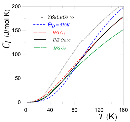
Figure 6: Lattice specific heat for YBa₂Cu₃O_7-x using the Debye model for $\Theta_{D}$ = 530 K and inelastic neutron scattering (INS) for three doping ${x}$. For comparison we add the the total specific heat experimental data (crosses) reported for YBa₂Cu₃O_6.92 by Bessergenev .

IV.2 Inelastic neutron scattering

An alternative way to use series and approximations is to appeal to the experimental phonon density of states (PDOS) reported by inelastic neutron scattering (INS) for YBa₂Cu₃O_7-x with several doping ${x}$ Renker88 . In their experiments, the authors use a non superconducting sample as a reference, such as YBa₂Cu₃O₆, which is also reported.

We extract the PDOS data for YBa₂Cu₃O_6.97, YBa₂Cu₃O₇ and YBa₂Cu₃O₆ from the curves given in Renker88 , introduce each one in Eq. (22) to perform the integrals numerically observing the correct handling of the units, and include the curves in Fig. 6. We are assuming that the use of this approach already takes into account the anharmonic terms, at least up to the temperature interval considered.

To magnify the difference among the lattice specific heat curves for different oxygen concentrations, we show in Fig. 7 the lattice specific heat over temperature for the same values used in Fig. 6, keeping in mind that this type of curve is the most used one for reporting electronic specific heat. It can bee seen that the differences between experimental results and theoretical curves are more noticeable in this form. At this point we would like to analize three features: the difference between the total experimental specific heat for YBa₂Cu₃O_6.92 and the lattice specific heat computed using the PDOS for $7-x=6.97$ at the transition point is around 30$\%$ in this graphic; however, the difference in the lattice specific heat between two adjacent superconducting dopages at the same point is quite small; and last, the lattice specific heat for $7-x=6$ is 10$\%$ lower at $T_{c}$ than that for the superconducting counterparts. On these bases we conjecture that using the YBa₂Cu₃O₆ compound as a reference for the specific heat of the lattice can be considered as a rough approximation.

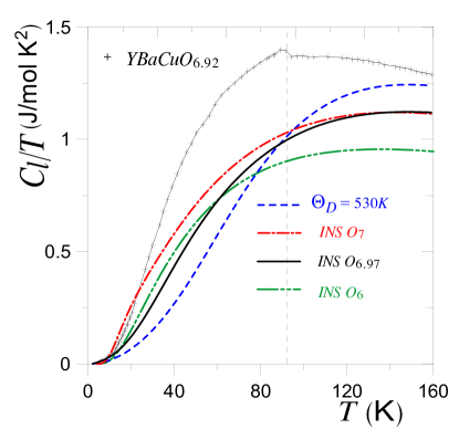
Figure 7: Specific heat over temperature of the phonons using the Debye model and Inelastic Neutron Scattering for the same values as in Fig. 6.

Above $T_{c}$ the lattice specific heat we obtain is still valid, but, as we mentioned before, our curve for the electronic specific heat is not strictly accurate, but only a guide.

By plotting the lattice specific heat $C_{l}/T$ vs $T^{2}$, we are able to reproduce the $T^{3}$ term observed in some experiments WangPhysRevB2001 . As we said above, this is true for the Debye model, as expected, but using the INS phonon density of states we find a $\beta$$T^{3}$ behavior for $T<$ 5 K with $\beta$ = 0.683 mJ/mol K⁴, compared to 0.305 and 0.392 reported in WangPhysRevB2001 and Moler97 respectively. Notice that our value of $\beta$ lies within the uncertainty of the INS experiment, and that unfortunately, no further experiments on PDOS for cuprates have been reported.

V Specific heat of YBa₂Cu₃O_6.92

We take the electronic specific heat we calculated for paired and unpaired electrons with the parameters $P_{0}=3\times 10^{5}$ and $f=0.018$, and add them to the lattice specific heat from the Debye model with $\Theta_{D}$ = 530 K and from the INS spectra for YBa₂Cu₃O_6.97, which we will be using in our calculations from now, and plot them in Figs. 8 and 9. Together with the total specific heat we plot the electronic specific heat (normal plus superconducting) for the purpose of emphasizing the size of its contribution.

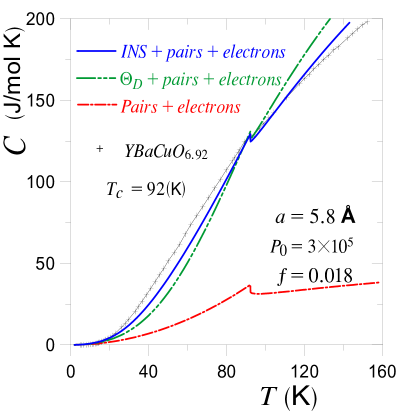
Figure 8: Total specific heat for YBa₂Cu₃O_6.92.

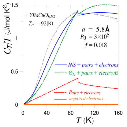
Figure 9: Total specific heat over temperature for YBa₂Cu₃O_6.92.

From these figures we may observe that the total height at the transition point for both, specific heat and specific heat over temperature, are reproduced by adding the three components we analized. However, we observe a minor difference between the experimental shape of the curve and ours below $T_{c}$, more remarkable in Fig. 9. This difference becomes more notorious around 40 K, where we believe that the contribution of the lattice $C_{l}$ needs a better analysis, supported by a more accurate experiment.

VI Conclusions

While most authors take the experimental curves of the total specific heat and subtract components, we are able to qualitatively construct the total specific heat for the YBa₂Cu₃O_7-x cuprates from a simple first principles model: the Boson-Fermion theory of superconductivity with the layered structure of HTSC. The model consists in taking the Cooper pairs as a boson gas coexisting with a unpaired electrons (or holes) Fermi gas, both gases under the confinement of the layered structure modeled by a Kronig-Penney potential in the Dirac comb limit in the perpendicular direction to the CuO₂. Although no interactions among bosons and no internal and/or external magnetic fields are considered, the model reproduces qualitatively well the experimental curves of the total specific heat.

A direct result is the critical temperature which depends on the anisotropy of the material, introduced through the planes impenetrability $P_{0}$ and the separation $a$ between them. Since we assumed that not all the pairable fermions are paired, this critical temperature also depends on the fraction of fermions that formed Cooper pairs. The total specific heat is calculated by including the specific heat coming from the bosons (superconducting electronic specific heat), unpaired fermions (normal electronic specific heat) and the lattice. The resulting curve is compared to that of YBa₂Cu₃O_6.92, which at $T_{c}$ = 92.2 K has a jump $\Delta C/T_{c}$ = 20 mJ/mol K² and is characterized by a linear dependence on temperature $\gamma_{e}T$ and a quadratic one $\alpha T^{2}$. These last two features are reproducible with our model by fixing the parameters $P_{0}$ and $f$ with the known values of $T_{c}$ and $\Delta C/T_{c}$ at $T_{c}$. The values we get for the constants $\gamma_{e}=$ 5.2 mJ/mol K² and $\alpha$ = 4.3 mJ/mol K³ are of the order of the experimentally reported ones. We also show their correspondence with the normal electronic specific heat coming from the unpaired fermions, and the superconducting term from the paired fermions, respectively. At the same time, these two results make plausible the assumption that not all pairable fermions in the Fermi sea were paired, even at temperatures near zero, and that the jump is a consequence of the condensation of the pairs. We also show that a simple Debye model for the lattice specific heat fails, as expected, but considering the results from INS experiments gives a better, albeit not perfect, approximation. A closer shape of our lattice specific heat to the experimental one should be obtained using data from a more accurate INS experiment. It can also be seen that the lattice specific heat shows the same temperature cubic behavior for $T<$ 5 K as experiments show WangPhysRevB2001 .

Another important result of our analysis is that the electronic specific heat (normal plus superconducting ) has a contribution of $30-40\%$ of the total at the transition temperature, and not only the $1-2\%$ most authors consider, which is of the order of the specific heat of the unpaired fermions alone. We suggest that when they subtract what they consider the lattice specific heat from a sample, either constructed by fits or using a non-superonducting reference material, they might be taking away a representative part of the total electronic specific heat.

Finally, we indirectly confirm that the upturn in the total specific heat at very low temperature is not a result of paired or unpaired fermions in the absence of a internal or external magnetic field. However, including magnetic terms should be a starting point for future study.

We acknowledge the partial support from grants CONACyT 104917 and PAPIIT IN-111070 and IN-105011.

References

- (1) G. Bednorz and K. A. Müller, Z. Phys. B. 64, 1175 (1986).
- (2) J. Bardeen, L. N. Cooper and J. R. Schrieffer, Phys. Rev. 108, 189 (1957).
- (3) C. P. Poole Jr., H. A. Farach, R. J. Creswick, R. Prozorov, Superconductivity, 2nd Ed. (Elsevier, The Netherlands, 2007).
- (4) Y. Wang, B. Revaz, A. Erb and A. Junod, Phys. Rev. B 63, 094508 (2001).
- (5) R. A. Fisher, J. E. Gordon and N. E. Phillips, Handbook of High-Temperature Superconductivity, Theory and Experiment,edited by J. Rober Schrieffer (Springer, 2007).
- (6) D. A. Wright, J. P. Emerson, B. F. Woodfield, J. E. Gordon, R. A. Fisher and N. E. Phillips, Phys. Rev. Lett 82, 1550 (1999).
- (7) K. A. Moler, D. L. Sisson, J. S. Urbach, M. R. Beasley, A. Kapitulnik, D. J. Baar, R. Liang and W. N. Hardy, Phys. Rev. B 55, 3954 (1997).
- (8) D. A. Wright, J. P. Emerson, B. F. Woodfield, S. F. Reklis, J. E. Gordon, R. A. Fisher and N. E. Phillips, J. Low Temp. Phys. 105, 897 (1996).
- (9) A. Junod, M. Roulin, J. Y. Genoud, B. Revaz, A. Erb, E. Walker, Physica C 275, 245 (1997).
- (10) R. A. Fisher, J. E. Gordon, S. Kim, N. E. Phillips and M. Stacy, Physica C 153, 1092 (1988).
- (11) Ch. Kittel, Introduction to Solid State Physics, 2nd Ed. (John Wiley and Sons, New York, 1965).
- (12) D. Varshney, R. K. Singh and A.K. Khaskalam, Phys. Stat. Sol. B 206, 749 (1998).
- (13) S. E. Inderhees, M. B. Salamon, T. A. Friedmann, and D. M. Ginsberg, Phys. Rev. B 36, 2401 (1987).
- (14) A. Junod, D. Eckert, T. Graf, G. Triscone and J. Muller, Physica C 162, 1401 (1989).
- (15) G. Mozurkewich, M. B. Salamon, and S. E. Inderhees, Phys. Rev. B 46, 11914 (1992).
- (16) N. E. Phillips, R. A. Fisher and J. E. Gordon, Progress in Low Temperature Physics, Vol. XIII, edited by D. F. Brewer (Elsevier, The Netherlands, 1992) p267.
- (17) J. E. Gordon, M. L. Tan, R. A. Fisher and N. E. Phillips, Solid State Comm. 69, 625 (1989).
- (18) V. G. Bessergenev, Yu A. Kovalevskaya, V. N. Naumov, G. I. Frolova, Physica C 245, 36 (1995).
- (19) M. Roulin, A. Junod, and E. Walker, Physica C 260, 257 (1996).
- (20) M. Roulin, A. Junod, and E. Walker, Physica C 296, 137 (1998).
- (21) A. Junod, A. Erb and C. Renner, Physica C 317, 333 (1999).
- (22) J. W. Loram, K. A. Mirza, J. R. Cooper and W. Y. Liang, Phys. Rev. Lett. 71, 1740 (1993).
- (23) C. Meingast, A. Inaba, R. Heid, V. Pankoke, K-P Bohnen, W. Reichardt and T. Wolf., J. Phys. Soc. Jap. 78, 074706 (2009).
- (24) R. Shaviv, E. F. Westrum Jr., R. C. J. Brown, M. Sayer, X. Yu and R. D. Weir, J. Chem. Phys. 92, 6794 (1990).
- (25) P. W. Anderson, G. Baskaran, Z. Zou and T. Hsu, Phys. Rev. Lett. 58 2790 (1987).
- (26) C. Uher in Handbook of Superconductor Materials, Vol. I, edited by D. A. Cardwell and D. S. Ginley (Institute of Physics Publishing Ltd, Bristol and Philadelphia, 2003) p75.
- (27) B. Revaz, J.-Y. Genoud, A. Jounod, K. Neumaier, A. Erb and E. Walker, Phys. Rev. Lett. 80, 3364 (1998).
- (28) S. E. Inderhees, M. B. Salamon, J. P. Rice and D. M. Ginsberg, Phys. Rev. Lett. 66, 232 (1991).
- (29) R. Friedberg and T. D. Lee, Phys. Letters A 138, 423 (1989).
- (30) R. Friedberg and T. D. Lee, Phys. Rev. B 40, 6745 (1989).
- (31) M. Casas, N. J. Davidson, M. de Llano, T. A. Mamedov, A. Puente, R. M. Quick, A. Rigo, and M. A. Solís, Physica A 295, 425 (2001).
- (32) S. K. Adhikari, M. Casas, A. Puente, A. Rigo, M. Fortes, M. A. Solís, M. de Llano, A. A. Valladares and O. Rojo, Phys. Rev. B 62, 8671 (2000).
- (33) D. M. Eagles, Phys. Rev. 186, 456 (1969).
- (34) P. Salas, M. Fortes, M. de Llano, F. J. Sevilla, and M. A. Solís, J. of Low Temp. Phys. 159, 540 (2010).
- (35) P. Salas, F. J. Sevilla, M. Fortes, M. de Llano, A. Camacho, and M. A. Solís, Phy. Rev. A 82, 033632 (2010).
- (36) Y. J. Uemura, Physica B 374, 1 (2006).
- (37) S. K. Adhikari, M. Casas, A. Puente, A. Rigo, M. Fortes, M. A. Solís, M. de Llano, A. A. Valladares and O. Rojo, Physica C 341, 233 (2000).
- (38) B. Renker, F. Gompf, E. Gering, D. Ewert, H. Rietschel and A. Dianoux, Z. Phys. B 73, 309 (1988). B. Renker, F. Gompf, E. Gering, G. Roth, W. Reichardt, D. Ewert, H. Rietschel and H. Mutka, Z. Phys. B 71, 437 (1988).
- (39) R. de L. Kronig and W. G. Penney, Proc. Roy. Soc. (London), A 130, 499 (1930); D. A. McQuarrie, The Kronig-Penney Model: A Single Lecture Illustrating the Band Structure of Solids, Chem. Educator 1 , 1 (1996) S1430-4171(96)01003-5.
- (40) X-G Wen and R. Kan, Phys. Rev. B 37, 595 (1988).
- (41) R. K. Pathria, Statistical Mechanics, 2nd Ed. (Pergamon, Oxford, 1996).
- (42) F. J. Sevilla, M. Grether, M. Fortes, M. de Llano, O. Rojo, M. A. Solís and A. A. Valladares, J. Low Temp. Phys. 121, 281 (2000).
- (43) C. P. Poole, H. A. Farach, and R. J. Creswick, Superconductivity (Academic Press, Inc. London, U. K., 1995).
- (44) C. Meingast, O. Kraut, T. Wolf, H. Wuhl, A. Erb and G. Muller-Vogt, Phys. Rev. Lett. 67, 1634 (1991).
- (45) P. Nagel, V. Pasler and C. Meingast, Phys. Rev. Lett. 85, 2376 (2000).
- (46) J. D. Jorgensen, S. Pei, P. Lightfoot, D. G. Hinks, B. W. Veal, B. Dabrowski, A. P. Paulikas and R. Kleb, Phys. C 171, 93 (1990).
- (47) W. Y. Liang, J. W. Loram, K. A. Mirza, N. Athanassopoulou and J. R. Cooper, Physica C 263, 277 (1996).
- (48) V. N. Naumov, G. I. Frolova, E. B. Amitin, V. E. Fedorov, P. P. Samoilov, Physica C 262, 143 (1996).
- (49) A. Tari, The Specific Heat of Matter at Low Temperatures (Imperial College Press, London, 2003).