Sum-Rate Maximization with Minimum Power Consumption for MIMO DF Two-Way Relaying: Part I - Relay Optimization

Abstract

The problem of power allocation is studied for a multiple-input multiple-output (MIMO) decode-and-forward (DF) two-way relaying system consisting of two source nodes and one relay. It is shown that achieving maximum sum-rate in such a system does not necessarily demand the consumption of all available power at the relay. Instead, the maximum sum-rate can be achieved through efficient power allocation with minimum power consumption. Deriving such power allocation, however, is nontrivial due to the fact that it generally leads to a nonconvex problem. In Part I of this two-part paper, a sum-rate maximizing power allocation with minimum power consumption is found for MIMO DF two-way relaying, in which the relay optimizes its own power allocation strategy given the power allocation strategies of the source nodes. An algorithm is proposed for efficiently finding the optimal power allocation of the relay based on the proposed idea of relative water-levels. The considered scenario features low complexity due to the fact that the relay optimizes its power allocation without coordinating the source nodes. As a trade-off for the low complexity, it is shown that there can be waste of power at the source nodes because of no coordination between the relay and the source nodes. Simulation results demonstrate the performance of the proposed algorithm and the effect of asymmetry on the considered system.

I Introduction

Two-way relaying (TWR) has recently attracted significant interests [1]-[17]. Establishing bi-directional links between one relay and two source nodes, the information exchange between the source nodes can be accomplished in two time slots [1]. In the first time slot (first phase) the source nodes simultaneously transmit their messages to the relay while in the second time slot (second phase) the relay forwards the messages to the destinations. The first phase is called the multiple access (MA) phase while the second phase is the broadcasting (BC) phase of TWR. Compared to conventional one-way relaying, which needs four time slots for the information exchange between the source nodes, TWR can achieve a higher spectral efficiency [1].

As the performance of TWR depends on the transmit strategies of both the source nodes and the relay, optimizing the transmit strategies such as power allocation and beamforming is one of the main research interests in TWR. The transmit strategies of the relay and source nodes depend on the relaying scheme. Similar to one-way relaying, the relaying scheme in TWR can be amplify-and-forward (AF), decode-and-forward (DF), etc., depending on the manner that the received information is processed at the relay before it is forwarded to the destinations. In the AF TWR scheme, the relay amplifies and broadcasts the signals received from the source nodes while it also amplifies and forwards the noise at the relay. Sum-rate maximization for multiple-input multiple-output (MIMO) AF TWR in which the relay and the source nodes all occupy multiple antennas is investigated in [2]-[4], while a mean square error minimizing scheme for MIMO AF TWR is studied in [5]. For MIMO AF relaying, low-complexity sub-optimal solutions can be obtained through diagonalizing the MIMO channel based on the singular value decomposition (SVD) or the generalized SVD (GSVD) and thereby transferring the problem of beamforming/precoding to the problem of power allocation [3], [5]. Finding the optimal solution, on the other hand, usually requires iterative algorithms with high complexity [4], [5]. The main challenge in investigating AF TWR, especially AF MIMO TWR, is the strong coupling between the transmit strategies of the source nodes and the relay due to noise propagation. As the result of noise propagation, the optimization over the transmit strategies of the source nodes and the relay usually leads to nonconvex problems. For example, the information rate of the communication in either direction is a nonconvex function of the covariance/beamforming matrices of the sources and the relay [1].

Unlike AF relaying, DF relaying does not have the problem of noise propagation. As a result, DF TWR may achieve a better performance than AF TWR, especially at low signal-to-noise ratios (SNRs), at the cost of higher complexity. Moreover, optimizing the power allocation in DF relaying usually leads to convex problems (see for example [6] and [7]). DF TWR has been studied in [8]-[15]. The optimal power allocation for DF TWR is studied under a fairness constraint in [12]. The optimal time division between the MA and BC phases and the optimal distribution of the relay’s power for achieving weighted sum-rate maximization are studied in [13]. While the above two works assume a single antenna at both the sources and the relay, the case with multiple antennas at all nodes is investigated in [14]-[15]. The achievable rate region and the optimal transmit strategies of both the source nodes and the relay are studied in [14], where the relay’s optimal transmit strategy is found by two water-filling based solutions coupled by the relay’s power limit. The authors of [15] specifically investigate the optimal transmit strategy in the BC phase of the MIMO DF TWR. It is shown that there may exist different strategies that lead to the same point in the rate region. Given that TWR can achieve a high spectral efficiency, it is of interest to optimize the power allocation so that the TWR scheme achieves high spectral efficiency using minimum power consumption. Unlike AF TWR, in which the sum-rate can always be increased when the relay has more transmission power, the maximum sum-rate of DF TWR can be achieved without consuming all the available power at the relay. However, finding the sum-rate maximizing power allocation with minimum power consumption is no longer a convex problem in general. Part I of this two-part paper studies the problem of finding the optimal relay power allocation which minimizes the relay power consumption among all relay power allocations that achieve the maximum sum-rate for the MIMO DF TWR given the power allocation of the source nodes. For brevity, this problem is called the sum-rate maximization with minimum (relay) power consumption. The considered scenario is referred to as relay optimization scenario. The objective of Part I of this two-part paper is to find the optimal power allocation strategy of the relay in the relay optimization scenario. The contributions of this part are as follows.

First, we show that the considered problem of sum-rate maximization with minimum relay power consumption is nonconvex. As the minimization of the relay power consumption is considered, the problem becomes more complex and the method used for deriving the optimal relay power allocation strategy in [7] and [14] is no longer valid. We first prove the sufficient and necessary condition for a relay power allocation to be optimal in the considered relay optimization scenario. Then, based on this condition, we propose an efficient algorithm for finding the optimal solution. The proposed algorithm can obtain the optimal relay power allocation in several steps without iterations, i.e., low complexity is achieved.

Second, we show that while the relay optimization scenario has the advantage of low complexity, as a trade-off it may lead to a waste of power at the source nodes because of the lack of coordination between the source nodes and the relay. We analyze the solution of the relay optimization problem for different relay power limits and show that a waste of power at the source nodes happens when the relay has a power limit less than a certain threshold for each considered system configuration and the thresholds are also given.

Third, the effect of asymmetry on the considered MIMO DF TWR is analyzed and demonstrated. It has been observed in [16], [17] that the asymmetry on channel gain, relay’s location, etc., can cause a performance degradation in single-input single-output (SISO) TWR. We extend this to the MIMO case and show the effect of asymmetry in power limits and number of antennas at the source nodes through analysis and simulations.

The rest of the paper is organized as follows. Section II gives the system model of this work. The relay optimization problem is solved and the features of the solution are investigated in Section III. Simulation results are shown in Section IV, and Section V concludes the paper. Section VI “Appendix” provides proofs for some lemmas and all theorems.

II System Model

Consider a TWR with two source nodes and one relay, where source node $i\,(i=1,2)$ and the relay have $n_{i}$ and $n_{\rm{r}}$ antennas, respectively. In the MA phase, source node $i$ transmits signal $\mathbf{W}_{i}\mathbf{s}_{i}$ to the relay. Here $\mathbf{W}_{i}$ is the precoding matrix of source node $i$ and $\mathbf{s}_{i}$ is the complex Gaussian information symbol vector of source node $i$. The elements of $\mathbf{s}_{i},\forall i$ are independent and identically distributed with zero mean and unit variance. The channels from source node $i$ to the relay and from the relay to source node $i$ are denoted as $\mathbf{H}_{i\rm{r}}$ and $\mathbf{H}_{{\rm{r}}i}$, respectively. Receiver channel state information is assumed at both the relay and the source nodes, i.e., source node $i$ knows $\mathbf{H}_{{\rm{r}}i}$ and the relay knows $\mathbf{H}_{i\rm{r}},\forall i$. It is also assumed that the relay knows $\mathbf{H}_{{\rm{r}}i},\forall i$ by using either channel reciprocity or channel feedback. The received signal at the relay in the MA phase is

$$\mathbf{y}_{\rm r}=\mathbf{H}_{1\rm{r}}\mathbf{W}_{1}\mathbf{s}_{1}+\mathbf{H}_{2\rm{r}}\mathbf{W}_{2}\mathbf{s}_{2}+\mathbf{n}_{\rm{r}}$$ (1)

where $\mathbf{n}_{\rm{r}}$ is the noise at the relay with covariance matrix $\sigma_{\rm{r}}^{2}\mathbf{I}$ in which $\mathbf{I}$ denotes the identity matrix. The maximum transmission power of source node $i$ is limited to $P_{i}^{\rm max}$. Define the transmit covariance matrices $\mathbf{D}_{i}=\mathbf{W}_{i}\mathbf{W}_{i}^{\rm H},\forall i$, in which $(\cdot)^{\rm H}$ stands for the conjugate transpose, and let $\mathbf{D}=[\mathbf{D}_{1},\mathbf{D}_{2}]$. Then the sum-rate of the MA phase is bounded by [19]

$$\hskip 8.53581ptR^{\rm ma}(\mathbf{D})=\log{\bigg{|}\mathbf{I}\!+\!(\mathbf{H}_{1{\rm{r}}}\mathbf{D}_{1}\mathbf{H}_{1{\rm{r}}}^{\rm H}\!+\!\mathbf{H}_{2{\rm{r}}}\mathbf{D}_{2}\mathbf{H}_{2{\rm{r}}}^{\rm H})(\sigma_{{\rm{r}}}^{2})^{-1}\bigg{|}}$$ (2)

where $|\cdot|$ denotes determinant. In the BC phase, the relay decodes $\mathbf{s}_{1}$ and $\mathbf{s}_{2}$ from the received signal, re-encodes messages using superposition coding and transmits the signal

$$\mathbf{x}_{\rm{r}}=\mathbf{T}_{{\rm{r}}2}\mathbf{s}_{1}+\mathbf{T}_{{\rm{r}}1}\mathbf{s}_{2}$$ (3)

where $\mathbf{T}_{{\rm{r}}i}$ is the $n_{\rm{r}}\times n_{j}$ relay precoding matrix for relaying the signal from source node $j$ to source node $i$. The maximum transmission power of the relay is limited to $P_{\rm{r}}^{\rm max}$. Note that in addition to the above superposition coding, the Exclusive-OR (XOR) based network coding is also used at the relay in the literature [20]-[22]. While XOR based network coding may achieve a better performance than superposition coding, it relies on the symmetry of the traffic from the two source nodes. The asymmetry in the traffic in the two directions can lead to a significant degradation in the performance of XOR in TWR [21], [22]. As the general case of TWR is considered and there is no guarantee of traffic symmetry, the approach of symbol-level superposition is assumed here at the relay as it is considered in [1] and [13]. Moreover, for the MIMO case as considered in this work, the superposition scheme can take advantage of the MIMO channels. In the superposition scheme, the relay uses separate beamformers for the signals towards two directions, which guarantees that each transmitted signal is optimal (subject to the transmission power constraints) given its MIMO channel. This cannot be achieved if the relay uses XOR based network coding.

The received signal at source node $i$ is

$$\mathbf{y}_{i}^{\prime}=\mathbf{H}_{{\rm{r}}i}\mathbf{x}_{\rm{r}}+\mathbf{n}_{i}$$ (4)

where $\mathbf{n}_{i}$ is the noise at source node $i$ with covariance matrix $\sigma_{i}^{2}\mathbf{I}$. With the knowledge of $\mathbf{H}_{{\rm{r}}i}$ and $\mathbf{T}_{{\rm{r}}j}$, source node $i$ subtracts the self-interference $\mathbf{H}_{{\rm{r}}i}\mathbf{T}_{{\rm{r}}j}\mathbf{s}_{i}$ from the received signal and the equivalent received signal at source node $i$ is

$$\mathbf{y}_{i}=\mathbf{H}_{{\rm{r}}i}\mathbf{T}_{{\rm{r}}i}\mathbf{s}_{j}+\mathbf{n}_{i}.$$ (5)

Define $\mathbf{B}_{i}=\mathbf{T}_{{\rm{r}}i}\mathbf{T}_{{\rm{r}}i}^{\rm H},\forall i$ and let $\mathbf{B}=[\mathbf{B}_{1},\mathbf{B}_{2}]$. The sum-rate of the considered DF TWR can be written as [1], [13], [20]

$$R^{\rm tw}(\mathbf{B},\mathbf{D})=\frac{1}{2}\min\{R^{\rm ma}(\mathbf{D}),R(\mathbf{B},\mathbf{D})\}$$ (6)

where

$$R(\mathbf{B},\mathbf{D})=\min\{\hat{R}_{{\rm{r}}1}(\mathbf{B}_{1}),\bar{R}_{2{\rm{r}}}(\mathbf{D}_{2})\}\qquad$$

$$\qquad+\min\{\hat{R}_{{\rm{r}}2}(\mathbf{B}_{2}\!),\bar{R}_{1{\rm{r}}}(\mathbf{D}_{1}\!)\},$$ (7)

in which

$$\bar{R}_{j{\rm{r}}}(\mathbf{D}_{j})=\log{|\mathbf{I}+(\mathbf{H}_{j{\rm{r}}}\mathbf{D}_{j}\mathbf{H}_{j{\rm{r}}}^{\rm H})(\sigma_{{\rm{r}}}^{2})^{-1}|},$$ (8)

and

$$\hat{R}_{{\rm{r}}i}(\mathbf{B}_{i})=\log|\mathbf{I}+(\mathbf{H}_{{\rm{r}}i}\mathbf{B}_{i}\mathbf{H}_{{\rm{r}}i}^{\rm H})(\sigma_{i}^{2})^{-1}|.$$ (9)

For brevity of presentation, we define the following sum-rate of the BC phase

$$R^{\rm bc}(\mathbf{B})=\hat{R}_{{\rm{r}}1}(\mathbf{B}_{1})+\hat{R}_{{\rm{r}}2}(\mathbf{B}_{2})$$ (10)

to represent the summation in the above equation hereafter.

For the relay optimization scenario considered here, the relay maximizes the sum-rate in (6) using minimum transmission power given the power allocation strategies of the source nodes. Since the relay needs to know $\mathbf{W}_{1}$ and $\mathbf{W}_{2}$ for decoding $\mathbf{s}_{1}$ and $\mathbf{s}_{2}$, respectively, as well as for designing $\mathbf{T}_{\mathrm{r}1}$ and $\mathbf{T}_{\mathrm{r}2}$, the source nodes should send their respective precoding matrices to the relay after they decide their transmit strategies. Similarly, the relay should also send $\mathbf{T}_{\mathrm{r}1}$ and $\mathbf{T}_{\mathrm{r}2}$ to both source nodes.

Given the above system model, we next solve the relay optimization problem.

III Relay optimization

In the relay optimization scenario, the relay and the source nodes do not coordinate in choosing their respective power allocation strategies. Instead, the relay aims at maximizing $R^{\rm tw}(\mathbf{B},\mathbf{D})$ in (6) with minimum power consumption after the source nodes decide their strategies and inform the relay.

Denote the power allocation that the source nodes decide to use as $\mathbf{D}^{0}=[\mathbf{D}_{1}^{0},\mathbf{D}_{2}^{0}]$. For maximizing the sum-rate given $\mathbf{D}^{0}$, the relay solves the following optimization problem

$$\mathop{\mathbf{max}}\limits_{\mathbf{B}}\quad R^{\rm tw}(\mathbf{B},\mathbf{D}^{0})$$ (11a)

$$\;\;\mathbf{s.t.}\quad\;\text{Tr}\{\mathbf{B}_{1}+\mathbf{B}_{2}\}\leq P_{\rm r}^{\rm max}.$$ (11b)

The problem (11) is convex. However, in order to find the optimal $\mathbf{B}$ with minimum $\text{Tr}\{\mathbf{B}_{1}+\mathbf{B}_{2}\}$ among all possible $\mathbf{B}$’s that achieve the same maximum of the objective function in (11), extra constraints need to be considered. Two necessary constraints are

$$\hat{R}_{{\rm r}i}(\mathbf{B}_{i})\leq\bar{R}_{j{\rm r}}(\mathbf{D}_{j}^{0}),\forall i$$ (12a)

$$R(\mathbf{B},\mathbf{D}^{0})\leq R^{\rm ma}(\mathbf{D}^{0}).$$ (12b)

The constraint (12a) is necessary because, due to the expression of $R(\mathbf{B},\mathbf{D})$ in (II), the power consumption of the relay can be reduced without decreasing the sum-rate $R^{\rm tw}(\mathbf{B},\mathbf{D})$ in (6) given $\mathbf{D}^{0}$ by reducing $\text{Tr}\{\mathbf{B}_{i}\}$ if $\hat{R}_{\mathrm{r}i}(\mathbf{B}_{i})>\bar{R}_{j\mathrm{r}}(\mathbf{D}_{j}^{0})$. Note that (12a) is not necessarily satisfied with equality at optimality. In fact, it can be shown that (12a) should be satisfied with inequality for at least one $i$ at optimality using subsequent results in Section III-B. It can also be shown that (12a) can be satisfied with inequalities for both $i$’s at optimality even if the relay has an unlimited power budget. We stress that (12a) is not sufficient for obtaining the optimal solution. Other constraints are also needed including (12b). The constraint (12b) is also necessary because if it is not satisfied given $\mathbf{D}^{0}$, then the power consumption of the relay can be reduced without decreasing the sum-rate $R^{\rm tw}(\mathbf{B},\mathbf{D}^{0})$ by decreasing $R(\mathbf{B},\mathbf{D}^{0})$ so that $R(\mathbf{B},\mathbf{D}^{0})=R^{\rm ma}(\mathbf{D}^{0})$.

The constraints in (12) make the considered problem nonconvex. The objective in this section is to find an efficient method of deriving the optimal power allocation of the relay in the considered scenario of relay optimization. It is straightforward to see that the power allocation of the relay should be based on waterfilling for relaying the signal in either direction regardless of how the relay distributes its power between relaying the signals in the two directions. This is due to the fact that the BC phase is interference free since both source nodes are able to subtract their self-interference. If the objective were to maximize $R^{\rm bc}(\mathbf{B})$ instead of $R^{\rm tw}(\mathbf{B},\mathbf{D}^{0})$, the optimal strategy of the relay could be found via a simple search. Indeed, in that case, we could find the optimal power allocation of the relay and consequently the optimal $\mathbf{B}$ by searching for the optimal proportion that the relay distributes its power between relaying the signals in the two directions. However, such approach is infeasible for the considered problem. The reason is that first of all it is unknown what is the total power that the relay uses in the optimal solution. As power efficiency is also considered, the relay may not use full power in its optimal strategy. Moreover, from the expression of $R^{\rm tw}(\mathbf{B},\mathbf{D})$ in (6), it can be seen that the maximum achievable $R^{\rm tw}(\mathbf{B},\mathbf{D}^{0})$ also depends on $\bar{R}_{1{\rm r}}(\mathbf{D}_{1}^{0})$, $\bar{R}_{2{\rm r}}(\mathbf{D}_{2}^{0})$, and $R^{\rm ma}(\mathbf{D}^{0})$. Due to this dependence, the two constraints in (12) are necessary for the considered problem of sum-rate maximization with minimum power consumption. However, these two constraints are implicit in the sense that they are constraints on the rates instead of on the power allocation of the relay. Such constraints offer no insight in finding the optimal $\mathbf{B}$. In order to transform the above mentioned dependence of $R^{\rm tw}(\mathbf{B},\mathbf{D}^{0})$ on $\bar{R}_{1{\rm r}}(\mathbf{D}_{1}^{0})$, $\bar{R}_{2{\rm r}}(\mathbf{D}_{2}^{0})$, and $R^{\rm ma}(\mathbf{D}^{0})$ into an explicit form, and to discover the insight behind the constraints in (12), we next propose the idea of relative water-levels and develop a method based on this idea.

III-A Relative water-levels

Denote the rank of $\mathbf{H}_{{\rm r}i}$ as $\mathrm{r}_{{\rm r}i}$ and the singular value decomposition (SVD) of $\mathbf{H}_{{\rm r}i}$ as $\mathbf{U}_{{\rm r}i}\mathbf{\Omega}_{{\rm r}i}\mathbf{V}_{{\rm r}i}^{\mathrm{H}}$. Assume that the first $\mathrm{r}_{{\rm r}i}$ diagonal elements of $\mathbf{\Omega}_{{\rm r}i}$ are non-zero, sorted in descending order and denoted as $\omega_{{\rm r}i}(1),\dots,\omega_{\mathrm{r}i}({\rm r}_{{\rm r}i})$, while the last $\min\{n_{i},n_{\rm r}\}-r_{{\rm r}i}$ diagonal elements are zeros. Define $\mathcal{I}_{i}=\{1,\dots,{\rm r}_{{\rm r}i}\},\forall i$ and $\alpha_{i}(k)={|\omega_{{\rm r}i}(k)|^{2}}/{\sigma_{i}^{2}},\forall k\in\mathcal{I}_{i},\forall i$. For a given $\mathbf{D}=[\mathbf{D}_{1},\mathbf{D}_{2}]$, define $\mu_{1}(\mathbf{D}_{1})$, $\mu_{2}(\mathbf{D}_{2})$, and $\mu_{\rm ma}(\mathbf{D})$ such that

$$\sum\limits_{k\in\mathcal{I}_{2}}\log\bigg{(}1+\big{(}\frac{1}{\mu_{1}(\mathbf{D}_{1})}\alpha_{2}(k)-1\big{)}^{+}\bigg{)}=\bar{R}_{1{\rm r}}(\mathbf{D}_{1})$$ (13a)

$$\sum\limits_{k\in\mathcal{I}_{1}}\log\bigg{(}1+\big{(}\frac{1}{\mu_{2}(\mathbf{D}_{2})}\alpha_{1}(k)-1\big{)}^{+}\bigg{)}=\bar{R}_{2{\rm r}}(\mathbf{D}_{2})$$ (13b)

$$\sum\limits_{i}\!\sum\limits_{k\in\mathcal{I}_{i}}\!\log\bigg{(}\!1+\big{(}\frac{1}{\mu_{\rm ma}(\mathbf{D})}\alpha_{i}(k)-1\big{)}^{+}\!\bigg{)}\!=R^{\rm ma}(\mathbf{D})$$ (13c)

where $(\cdot)^{+}$ stands for projection to the positive orthant. The physical meaning of $\mu_{i}(\mathbf{D}_{i})$ is that if waterfilling is performed on $\omega_{\mathrm{r}j}(k)$’s, $\forall k\in\mathcal{I}_{j}$ using the water-level $1/\mu_{i}(\mathbf{D}_{i})$, then the information rate of the transmission from the relay to source node $j$ using the resulting waterfilling-based power allocation achieves precisely $\bar{R}_{i\mathrm{r}}(\mathbf{D}_{i})$. The physical meaning of $\mu_{\rm ma}(\mathbf{D})$ is that if waterfilling is performed on $\omega_{\mathrm{r}i}(k)$’s, $\forall k\in\mathcal{I}_{i},\forall i$ using the water-level $1/\mu_{\rm ma}(\mathbf{D})$, then the sum-rate of the transmission from the relay to the two source nodes using the resulting waterfilling-based power allocation achieves precisely ${R}^{\rm ma}(\mathbf{D})$. Note that $1/\mu_{i}(\mathbf{D}_{i}),\forall i$ and $1/\mu_{\rm m}(\mathbf{D})$ are not the actual water-levels for the MA or the BC phase. They are just relative water-levels introduced to transfer and simplify the constraints in (12). Denote the actual water-levels used by the relay for relaying the signal from source node $j$ to source node $i$ as $1/\lambda_{i},\forall i$. With water-level $1/\lambda_{i}$, $\mathbf{B}_{i}$ can be given as $\mathbf{B}_{i}=\mathbf{V}_{\mathrm{r}i}\mathbf{P}_{\mathrm{r}i}(\lambda_{i})\mathbf{V}_{\mathrm{r}i}^{\mathrm{H}}$ where $\mathbf{P}_{\mathrm{r}i}(\lambda_{i})=\text{diag}\bigg{(}\big{(}\frac{1}{\lambda_{i}}-\frac{1}{\alpha_{i}(1)}\big{)}^{+},\dots,\big{(}\frac{1}{\lambda_{i}}\!-\!\frac{1}{\alpha_{i}(\mathrm{r}_{\mathrm{r}i})}\big{)}^{+},0,\dots,0\bigg{)}$ in which $\text{diag}(\cdot)$ stands for making a diagonal matrix using the given elements, $(\cdot)^{+}$ stands for projection to the positive orthant, and $\mathbf{0}_{n_{\mathrm{r}}-\mathrm{r}_{\mathrm{r}i}}$ stands for all-zero matrix of size $(n_{\mathrm{r}}-\mathrm{r}_{\mathrm{r}i})\times(n_{\mathrm{r}}-\mathrm{r}_{\mathrm{r}i})$. The power allocated on $\omega_{\mathrm{r}i}(k)$ is $p_{\mathrm{r}i}(k)=\big{(}{1}/{\lambda_{i}}-{1}/{\alpha_{i}(k)}\big{)}^{+},\forall k\in\mathcal{I}_{i},\forall i$. The resulting rate $\hat{R}_{\mathrm{r}i}(\mathbf{B}_{i})$ is given by $\sum\limits_{k\in\mathcal{I}_{i}}\!\log\!\bigg{(}\!1\!+\!\big{(}{\alpha_{i}(k)}/{\lambda_{i}}-\!1\big{)}^{+}\!\bigg{)}$. Using $\mu_{1}(\mathbf{D}_{1})$, $\mu_{2}(\mathbf{D}_{2})$, and $\mu_{\rm ma}(\mathbf{D})$, the constraints in (12a) can be rewritten as

$$\lambda_{i}\geq\mu_{j}(\mathbf{D}_{j}^{0}),\forall i\quad\quad\quad\quad\quad\quad\;\,$$ (14a)

$$\sum\limits_{i}\sum\limits_{k\in\mathcal{I}_{i}}\!\log\!\bigg{(}\!1\!+\!\big{(}\frac{1}{\lambda_{i}}\alpha_{i}(k)-\!1\big{)}^{+}\!\bigg{)}\quad\quad\quad\quad\quad\quad\quad\;\,$$

$$\leq\sum\limits_{i}\sum\limits_{k\in\mathcal{I}_{i}}\!\log\!\bigg{(}\!1\!+\!\big{(}\frac{1}{\mu_{\mathrm{ma}}(\mathbf{D}^{0})}\alpha_{i}(k)-\!1\big{)}^{+}\!\bigg{)}.$$ (14b)

Given (13a) and (13b), it is not difficult to see that (12a) is equivalent to (14a). Moreover, the equivalence between (12b) and (14b) can be explained as follows. Given $\mathbf{D}^{0}$ and (12b), $R^{\rm tw}(\mathbf{B},\mathbf{D}^{0})$ in (11a) becomes $R(\mathbf{B},\mathbf{D}^{0})/2$. Given (12a), or equivalently (14a), $R(\mathbf{B},\mathbf{D})$ in (II) with $\mathbf{D}=\mathbf{D}^{0}$ becomes $\hat{R}_{{\rm{r}}1}(\mathbf{B}_{1})+\hat{R}_{{\rm{r}}2}(\mathbf{B}_{2})$. Then, substituting the left-hand side of (12b) with $\hat{R}_{{\rm{r}}1}(\mathbf{B}_{1})+\hat{R}_{{\rm{r}}2}(\mathbf{B}_{2})$, i.e., $R^{\rm bc}(\mathbf{B})$ in (10), and using (13c), the constraint (14b) is obtained.

The procedure for the relay optimization can be summarized in the following three steps:

1. Obtain $\mu_{1}(\mathbf{D}_{1}^{0})$, $\mu_{2}(\mathbf{D}_{2}^{0})$, and $\mu_{\mathrm{ma}}(\mathbf{D}^{0})$ from $\mathbf{D}^{0}$;

2. Determine the optimal $\lambda_{i}$;

3. Obtain $\mathbf{P}_{\mathrm{r}i}(\lambda_{i})$ and $\mathbf{B}_{i}$ from $\lambda_{i}$.

The first and the third steps are straightforward given the definitions (13a)-(13c) and (LABEL:e:WL2PW). Therefore, finding the optimal $\lambda_{i},\forall i$ in the second step is the essential part to be dealt with later in this section.

From hereon, $\mu_{1}(\mathbf{D}_{1})$, $\mu_{2}(\mathbf{D}_{2})$, and $\mu_{\rm ma}(\mathbf{D})$ are denoted as $\mu_{1}$, $\mu_{2}$ and $\mu_{\mathrm{ma}}$, respectively, for brevity. The same markers/superscripts on $\mathbf{D}_{i}$ and/or $\mathbf{D}$ are used on $\mu_{i}$ and/or $\mu_{\mathrm{ma}}$ to represent the connection. For example, $\mu_{i}(\mathbf{D}_{i}^{0})$ and $\mu_{\mathrm{ma}}(\tilde{\mathbf{D}})$ are briefly denoted as $\mu_{i}^{0}$ and $\tilde{\mu}_{\mathrm{ma}}$, respectively. The rate $\hat{R}_{\mathrm{r}i}(\mathbf{B}_{i})$ obtained using water-level $1/\lambda_{i}$ is also denoted as $\hat{R}_{\mathrm{r}i}(\lambda_{i})$.

III-B Algorithm for relay optimization

Using the relative water-levels $\mu_{i},\forall i$ and $\mu_{\rm ma}$, we can now develop the algorithm for relay optimization. In order to do that, the following lemmas are presented.

Lemma 1: $1/\mu_{\rm ma}<\max\{1/\mu_{1},1/\mu_{2}\}$.

Proof: The proof for Lemma 1 is straightforward. Using (13a)-(13c), it can be seen that $R^{\rm ma}(\mathbf{D})\geq\sum\limits_{i}\bar{R}_{i\mathrm{r}}(\mathbf{D}_{i})$ if $1/\mu_{\rm ma}\geq\max\{1/\mu_{1},1/\mu_{2}\}$. However, given the definitions in (2) and (8), it can be seen that $R^{\rm ma}(\mathbf{D})\geq\sum\limits_{i}\bar{R}_{i\mathrm{r}}(\mathbf{D}_{i})$ is impossible [19]. Therefore, $1/\mu_{\rm ma}<\max\{1/\mu_{1},1/\mu_{2}\}$. $\blacksquare$

Lemma 2: Assume that there exist $\{\lambda_{i},\lambda_{j}\}$ and $\{\lambda_{i}^{\prime},\lambda_{j}^{\prime}\}$ such that $\lambda_{i}^{\prime}<\lambda_{i}\leq\lambda_{j}<\lambda_{j}^{\prime}$. If $\sum\limits_{l}\text{Tr}\{\mathbf{P}_{\mathrm{r}l}(\lambda_{l})\}=\sum\limits_{l}\text{Tr}\{\mathbf{P}_{\mathrm{r}l}(\lambda_{l}^{\prime})\}$, then $\sum\limits_{l}\hat{R}_{\mathrm{r}l}(\lambda_{l})>\sum\limits_{l}\hat{R}_{\mathrm{r}l}(\lambda_{l}^{\prime})$ as long as $1/\lambda_{j}>\min\limits_{k}\{1/\alpha_{j}(k)\}$.

Proof: See Subsection VI-A in Appendix. $\blacksquare$

Lemma 2 states that, for any given $\{\lambda_{1},\lambda_{2}\}$ such that $1/\lambda_{2}>\min\limits_{k}\{1/\alpha_{2}(k)\}$ assuming $\lambda_{1}\leq\lambda_{2}$, decreasing $\min\{\lambda_{1},\lambda_{2}\}$ and increasing $\max\{\lambda_{1},\lambda_{2}\}$ while fixing the total power consumption leads to a smaller BC phase sum-rate than that achieved by using $\{\lambda_{1},\lambda_{2}\}$.

Lemma 3: Assume that there exist $\{\lambda_{i},\lambda_{j}\}$ and $\{\lambda_{i}^{\prime},\lambda_{j}^{\prime}\}$ such that $\lambda_{i}<\lambda_{j}$, $\lambda_{i}^{\prime}>\lambda_{i}$ and $\lambda_{j}^{\prime}>\lambda_{j}$, and

$$\hat{R}_{\mathrm{r}i}(\lambda_{i}^{\prime})+\hat{R}_{\mathrm{r}j}(\lambda_{j})=\hat{R}_{\mathrm{r}i}(\lambda_{i})+\hat{R}_{\mathrm{r}j}(\lambda_{j}^{\prime})$$ (15)

then as long as $\lambda_{i}^{\prime}\leq\lambda_{j}$, it holds true that

$$\text{Tr}\{\mathbf{P}_{\mathrm{r}i}(\lambda_{i}^{\prime})\}+\text{Tr}\{\mathbf{P}_{\mathrm{r}j}(\lambda_{j})\}<\text{Tr}\{\mathbf{P}_{\mathrm{r}i}(\lambda_{i})\}+\text{Tr}\{\mathbf{P}_{\mathrm{r}j}(\lambda_{j}^{\prime})\}.$$ (16)

Proof: See Subsection VI-B in Appendix. $\blacksquare$

Lemma 3 states that, for any given $\{\lambda_{1},\lambda_{2}\}$, decreasing $\min\{\lambda_{1},\lambda_{2}\}$ and increasing $\max\{\lambda_{1},\lambda_{2}\}$ such that the BC phase sum-rate is unchanged, the power consumption increases.

Theorem 1: The optimal solution of the considered relay optimization problem always satisfies the following properties

$$\min\bigg{\{}\frac{1}{\lambda_{1}},\frac{1}{\lambda_{2}}\bigg{\}}=\min\bigg{\{}\frac{1}{\mu_{1}^{0}},\frac{1}{\mu_{2}^{0}}\bigg{\}}\quad\text{if}\quad\lambda_{1}\neq\lambda_{2}\;$$ (17a)

$$\frac{1}{\lambda_{1}}=\frac{1}{\lambda_{2}}=\min\bigg{\{}\frac{1}{\mu_{\rm ma}^{0}},\frac{1}{\lambda^{0}}\bigg{\}}\quad\text{if}\quad\lambda_{1}=\lambda_{2}\qquad$$ (17b)

in which ${1}/{\lambda^{0}}$ is the water-level obtained by waterfilling $P_{\mathrm{r}}^{\rm max}$ on $\omega_{\mathrm{r}i}(k),\forall k\in\mathcal{I}_{i},\forall i$.

Proof: See Subsection VI-C in Appendix. $\blacksquare$

According to the proof of Theorem 1, it can be seen that $\lambda_{1}\neq\lambda_{2}$ at optimality and consequently the equation in (17a) holds when both of the following two conditions are satisfied: (i) the relay has sufficient power, i.e., $1/\lambda^{0}>\min\{1/\mu_{1}^{0},1/\mu_{2}^{0}\}$, and (ii) there is asymmetry between $\mu_{1}^{0}$ and $\mu_{2}^{0}$, i.e., $\min\{1/\mu_{1}^{0},1/\mu_{2}^{0}\}<1/\mu_{\rm ma}^{0}<\max\{1/\mu_{1}^{0},1/\mu_{2}^{0}\}$. If either of the above two conditions is not satisfied, $\lambda_{1}=\lambda_{2}$ at optimality and consequently the equation in (17b) holds.

Theorem 2: The conditions (14a), (14b), (17a), and (17b) are sufficient and necessary to determine the optimal $\{\lambda_{1},\lambda_{2}\}$ with minimum power consumption for the relay optimization problem among all $\{\lambda_{1},\lambda_{2}\}$’s that maximize the sum-rate $R^{\rm tw}(\mathbf{B},\mathbf{D}^{0})$.

Proof: See Subsection VI-D in Appendix. $\blacksquare$

It should be noted that the power constraint (11b) is not always tight at optimality due to the constraints in (14a), (14b) (or equivalently (12a), (12b)), (17a), and (17b). Each of (14a), (14b), (17a), and (17b) may refrain the relay from using its full power at optimality. The reason can be found from the proofs of Theorems 1 and 2. Specifically, (14a) and (17a) make sure that there is no superfluous power spent for relaying the signal in each direction while (14b) and (17b) guarantee that the power consumption of the relay cannot be further reduced without reducing the sum-rate.

TABLE I: The algorithm for relay optimization.

1. Initial waterfilling: allocate $P_{\mathrm{r}}^{\rm max}$ on $\omega_{\mathrm{r}i}(k),\forall k\in\mathcal{I}_{i},\forall i$ using waterfilling. Denote the initial water level as ${1}/{\lambda^{0}}$. Set ${1}/{\lambda_{1}}={1}/{\lambda_{2}}={1}/{\lambda^{0}}$. The power allocated on $\omega_{\mathrm{r}i}(k)$ is $p_{\mathrm{r}i}(k)=\big{(}{1}/{\lambda_{i}}-{1}/{\alpha_{i}(k)}\big{)}^{+},\forall k\in\mathcal{I}_{i},\forall i$.
2. Check if ${1}/{\lambda_{i}}\leq 1/\mu_{j}^{0}$ for both $i=1,2$. If yes, proceed to Step 6. Otherwise, assume that ${1}/{\lambda_{1}}>1/\mu_{2}^{0}$, proceed to Step 3.
3. Set $\lambda_{1}=\mu_{2}^{0}$. Check if $1/\lambda_{2}<1/\mu_{1}^{0}$. If not, proceed to Step 4. Otherwise, proceed to Step 5.
4. Calculate $P_{\mathrm{r}}^{\prime}=P_{\mathrm{r}}^{\rm max}-\sum\limits_{k\in\mathcal{I}_{1}}{p_{\mathrm{r}1}(k)}$. Allocate $P_{\mathrm{r}}^{\prime}$ on $\omega_{\mathrm{r}2}(k)$’s,$\forall k\in\mathcal{I}_{2}$ via waterfilling. Obtain the water level $1/\lambda_{2}$. If $1/\lambda_{2}>1/\mu_{1}^{0}$, proceed to Step 5. Otherwise, go to Step 6.
5. Set $\lambda_{2}=\mu_{1}^{0}$ and proceed to Step 6.
6. If $1/\lambda_{i}\geq 1/\mu_{\mathrm{ma}}^{0},\forall i$, set $\lambda_{i}=\mu_{\mathrm{ma}}^{0},\forall i$. Check if $1/\lambda_{i}\leq 1/\mu_{\mathrm{ma}}^{0},\forall i$. If yes, output $\lambda_{i},\forall i$ and break. Otherwise, check if $\sum\limits_{i}\hat{R}_{\mathrm{r}i}(\lambda_{i})\leq R^{\rm ma}(\mathbf{D}^{0})$. If yes, output $\lambda_{i},\forall i$ and break. Otherwise, proceed to Step 7.
7. Assuming that $\lambda_{j}<\lambda_{i}$, find $\lambda_{j}^{\prime}$ such that $|\mathcal{M}_{\mathrm{r}j}^{+}|\log\lambda_{j}^{\prime}=\sum\limits_{k\in\mathcal{M}_{\mathrm{r}j}^{+}}\log\alpha_{j}(k)-R^{\rm ma}(\mathbf{D}^{0})+\bar{R}_{j\mathrm{r}}(\mathbf{D}_{j}^{0})$, where $p_{\mathrm{r}j}(k)=\big{(}{1}/{\lambda_{j}^{\prime}}-{1}/{\alpha_{j}(k)}\big{)}^{+},\forall k\in\mathcal{I}_{j}$, $\mathcal{M}_{\mathrm{r}j}^{+}=\{k|p_{\mathrm{r}j}(k)>0\}$ and $|\mathcal{M}_{\mathrm{r}j}^{+}|$ is the cardinality of the set $\mathcal{M}_{\mathrm{r}j}^{+}$. Set $\lambda_{j}=\lambda_{j}^{\prime}$ and output $\lambda_{i}$ and $\lambda_{j}$.

Based on the above results in Theorem 1 and Theorem 2, the algorithm summarized in Table I is proposed to find the optimal relay power allocation for the relay optimization problem. The algorithm can be briefly understood as follows. Step 1 performs initial power allocation and obtains the initial water level $\lambda^{0}$. The water-levels $\lambda_{i}=\lambda^{0},\forall i$ maximize $R^{\rm bc}(\mathbf{B})$ among all possible $\{\lambda_{1},\lambda_{2}\}$ combinations subject to the power limit of the relay. Step 2 checks if $\min\{\hat{R}_{{\rm{r}}i}(\mathbf{B}_{i}),\bar{R}_{j{\rm{r}}}(\mathbf{D}_{j})\}$ is upper-bounded by $\bar{R}_{j\mathrm{r}}(\mathbf{D}_{j}^{0}),\forall i$. If $\hat{R}_{\mathrm{r}1}(\lambda_{1}^{0})>\bar{R}_{2\mathrm{r}}(\mathbf{D}_{2}^{0})$, the relay reduces its transmission power allocated for relaying the signal from source node $2$ to source node $1$ so that $\hat{R}_{\mathrm{r}1}(\lambda_{1})=\bar{R}_{2\mathrm{r}}(\mathbf{D}_{2}^{0})$ in Step 3. In the case that $\hat{R}_{\mathrm{r}1}(\lambda_{1})$ is reduced in Step 3, in terms of increasing $\lambda_{1}$, extra power becomes available for relaying the signal from source node $1$ to source node $2$. Therefore, if $\hat{R}_{\mathrm{r}2}(\lambda_{2}^{0})<\bar{R}_{1\mathrm{r}}(\mathbf{D}_{1}^{0})$, the remaining power of the relay is allocated for relaying the signal from source node $1$ to source node $2$ at first in Step 4. Later in Step 4, it is checked if $\hat{R}_{\mathrm{r}2}(\lambda_{2})>\bar{R}_{1\mathrm{r}}(\mathbf{D}_{1}^{0})$ under the new power allocation. If $\hat{R}_{\mathrm{r}2}(\lambda_{2})>\bar{R}_{1\mathrm{r}}(\mathbf{D}_{1}^{0})$ in Step 4, the relay reduces its transmission power allocated for relaying the signal from source node $1$ to source node $2$ so that $\hat{R}_{\mathrm{r}2}(\lambda_{2})=\bar{R}_{1\mathrm{r}}(\mathbf{D}_{1}^{0})$ in Step 5. Steps 6 checks if $\hat{R}_{\mathrm{r}1}(\lambda_{1})+\hat{R}_{\mathrm{r}2}(\lambda_{2})\leq R^{\rm ma}(\mathbf{D}^{0})$. In the case that this constraint is not satisfied, Step 6 or Step 7 revise the power allocation so that $\hat{R}_{\mathrm{r}1}(\lambda_{1})+\hat{R}_{\mathrm{r}2}(\lambda_{2})=R^{\rm ma}(\mathbf{D}^{0})$ and the power consumption of the relay is minimized. The above procedure in the proposed algorithm, which terminates after Step 6 or 7, is not iterative.

The following theorem regarding the proposed algorithm is in order.

Theorem 3: The water-levels obtained using the algorithm for relay optimization in Table I achieve the optimal relay power allocation for the considered relay optimization problem of sum-rate maximization with minimum relay power consumption.

Proof: See Subsection VI-E in Appendix. $\blacksquare$

Depending on the source node power allocation strategies and the power limit at the relay, different results can be obtained at the output of the algorithm in Table I. Define the power thresholds $P_{\mathrm{ma}}=\sum\limits_{i}\sum\limits_{k\in\mathcal{I}_{i}}\big{(}{1}/{\mu_{\mathrm{ma}}^{0}}-{1}/{\alpha_{i}(k)}\big{)}^{+}$, $P_{\mathrm{l}}=\sum\limits_{i}\sum\limits_{k\in\mathcal{I}_{i}}\big{(}{1}/{\max\{\mu_{1}^{0},\mu_{2}^{0}\}}-{1}/{\alpha_{i}(k)}\big{)}^{+}$, $P_{\mathrm{t}}=\sum\limits_{i}\sum\limits_{k\in\mathcal{I}_{i}}\big{(}{1}/{\mu_{i}^{0}}-{1}/{\alpha_{i}(k)}\big{)}^{+}$ and $P_{\mathrm{s}}=\sum\limits_{i}\sum\limits_{k\in\mathcal{I}_{i}}\big{(}{1}/\min\{\mu_{1}^{0},\mu_{2}^{0}\}-{1}/{\alpha_{i}(k)}\big{)}^{+}$. Recall from Lemma 1 that $\mu_{\rm ma}^{0}>\min\{\mu_{1}^{0},\mu_{2}^{0}\}$.

For the case that $\mu_{\rm ma}^{0}\geq\max\{\mu_{1}^{0},\mu_{2}^{0}\}$, the following subcases exit as $P_{\mathrm{r}}^{\mathrm{max}}$ increases. If $P_{\mathrm{r}}^{\mathrm{max}}$ is small such that $P_{\mathrm{r}}^{\mathrm{\rm max}}<P_{\mathrm{\rm ma}}$, the algorithm proceeds through Steps 1-2-6 and

$$\quad\;\lambda_{i}=\lambda^{0}>\mu_{\mathrm{ma}}^{0},\forall i$$ (18a)

$$\sum\limits_{i}\text{Tr}\{\mathbf{P}_{\mathrm{r}i}(\lambda_{i})\}=P_{\mathrm{r}}^{\mathrm{max}}$$ (18b)

at the output of the algorithm, while (14a) and (14b) are satisfied with inequality. Note that some power of the source nodes is wasted in this subcase. Since the sum-rate $R^{\rm tw}(\mathbf{B},\mathbf{D})$ is bounded by $\hat{R}_{\mathrm{r}1}(\lambda_{1})+\hat{R}_{\mathrm{r}2}(\lambda_{2})$ due to the small power limit of the relay, the source nodes could use less power without reducing $R^{\rm tw}(\mathbf{B},\mathbf{D})$ if there would be coordination in the system. Indeed, if the source nodes could be coordinated to optimize their power allocation as well, they only need to use the power of $\text{Tr}\{\mathbf{D}^{\dagger}_{1}\}$+$\text{Tr}\{\mathbf{D}^{\dagger}_{2}\}$, where $\mathbf{D}^{\dagger}=[\mathbf{D}^{\dagger}_{1},\mathbf{D}^{\dagger}_{2}]$ is the optimal solution to the following problem

$$\mathop{\mathbf{min}}\limits_{\mathbf{D}}\;\text{Tr}\{\mathbf{D}_{1}\}+\text{Tr}\{\mathbf{D}_{2}\}$$ (19a)

$$\mathbf{\;\;s.t.}\;R^{\rm ma}(\mathbf{D})\geq\hat{R}_{\mathrm{r}1}(\lambda^{0})+\hat{R}_{\mathrm{r}2}(\lambda^{0})$$ (19b)

$$\qquad\;\bar{R}_{1\mathrm{r}}(\mathbf{D}_{1})\geq\hat{R}_{\mathrm{r}2}(\lambda^{0})$$ (19c)

$$\qquad\;\bar{R}_{2\mathrm{r}}(\mathbf{D}_{2})\geq\hat{R}_{\mathrm{r}1}(\lambda^{0}).$$ (19d)

It can be shown that $\text{Tr}\{\mathbf{D}^{0}_{1}\}+\text{Tr}\{\mathbf{D}^{0}_{2}\}>\text{Tr}\{\mathbf{D}^{\dagger}_{1}\}+\text{Tr}\{\mathbf{D}^{\dagger}_{2}\}$ in this subcase. Therefore, the power of $\text{Tr}\{\mathbf{D}^{0}_{1}\}+\text{Tr}\{\mathbf{D}^{0}_{2}\}-\text{Tr}\{\mathbf{D}^{\dagger}_{1}\}-\text{Tr}\{\mathbf{D}^{\dagger}_{2}\}$ is wasted at the source nodes because of the lack of coordination.

Increasing $P_{\mathrm{r}}^{\mathrm{max}}$ such that $P_{\mathrm{ma}}\leq P_{\mathrm{r}}^{\mathrm{max}}\leq P_{\mathrm{l}}$, the algorithm proceeds through Steps 1-2-6. Increasing $P_{\mathrm{r}}^{\mathrm{max}}$ such that $P_{\mathrm{l}}<P_{\mathrm{r}}^{\mathrm{max}}\leq P_{\mathrm{t}}$, the algorithm proceeds through Steps 1-2-3-4-6. Further increasing $P_{\mathrm{r}}^{\mathrm{max}}$ such that $P_{\mathrm{t}}<P_{\mathrm{r}}^{\mathrm{max}}\leq P_{\mathrm{s}}$, the algorithm proceeds through Steps 1-2-3-4-5-6. Further increasing $P_{\mathrm{r}}^{\mathrm{max}}$ such that $P_{\mathrm{r}}^{\mathrm{max}}>P_{\mathrm{s}}$, the algorithm proceeds through Steps 1-2-3-5-6. In the above subcases, it holds that

$$\quad\;\lambda_{i}=\mu_{\mathrm{ma}}^{0}\geq\lambda^{0},\forall i$$ (20a)

$$\sum\limits_{i}\text{Tr}\{\mathbf{P}_{\mathrm{r}i}(\lambda_{i})\}\leq P_{\mathrm{r}}^{\mathrm{max}}$$ (20b)

at the output of the algorithm, while (14a) is satisfied with inequality for each $i$ such that $1/\mu_{i}^{0}>1/\mu_{\mathrm{ma}}^{0}$ and (14b) is satisfied with equality. For these subcases, the sum-rate $R^{\rm tw}(\mathbf{B},\mathbf{D})$ is bounded by $R^{\rm ma}(\mathbf{D}^{0})$ and there is no waste of power at the source nodes.

For the case that $\mu_{\mathrm{ma}}^{0}<\max\{\mu_{1}^{0},\mu_{2}^{0}\}$, it holds that $\min\{\mu_{1}^{0},\mu_{2}^{0}\}<\mu_{\mathrm{ma}}^{0}<\max\{\mu_{1}^{0},\mu_{2}^{0}\}$ according to Lemma 1. Assume that $\mu_{2}^{0}>\mu_{1}^{0}$ and find $\bar{\lambda}_{2}$ such that $\hat{R}_{\mathrm{r}2}(\bar{\lambda}_{2})=R^{\rm ma}(\mathbf{D}^{0})-\bar{R}_{2\mathrm{r}}(\mathbf{D}_{2}^{0})$. Let $\bar{\lambda}_{1}=\mu_{2}^{0}$ and define $\bar{P}_{\mathrm{ma}}=\sum\limits_{i}\sum\limits_{k\in\mathcal{I}_{i}}\big{(}1/\bar{\lambda}_{i}-{1}/{\alpha_{i}(k)}\big{)}^{+}$. It can be seen from Lemma 3 that $\bar{P}_{\mathrm{ma}}>P_{\mathrm{ma}}$. The following subcases appear as $P_{\mathrm{r}}^{\mathrm{max}}$ increases. If $P_{\mathrm{r}}^{\mathrm{max}}$ is small such that $P_{\mathrm{r}}^{\mathrm{max}}<P_{\mathrm{l}}$, the algorithm proceeds through Steps 1-2-6 and

$$\lambda_{i}=\lambda^{0}>\max\{\mu_{1}^{0},\mu_{2}^{0}\},\forall i$$ (21a)

$$\;\sum\limits_{i}\text{Tr}\{\mathbf{P}_{\mathrm{r}i}(\lambda_{i})\}=P_{\mathrm{r}}^{\mathrm{max}}$$ (21b)

at the output of the algorithm, while (14a) and (14b) are satisfied with inequality. Increasing $P_{\mathrm{r}}^{\mathrm{max}}$ such that $P_{\mathrm{l}}\leq P_{\mathrm{r}}^{\mathrm{max}}\leq\bar{P}_{\mathrm{ma}}$, the algorithm proceeds through Steps 1-2-3-4-6 and

$$\quad\;\;\,\,\lambda_{1}=\mu_{2}^{0}\geq\lambda^{0}$$ (22a)

$$\sum\limits_{i}\text{Tr}\{\mathbf{P}_{\mathrm{r}i}(\lambda_{i})\}=P_{\mathrm{r}}^{\mathrm{max}}$$ (22b)

at the output of the algorithm, while (14a) is satisfied with equality for $i=1$ and inequality for $i=2$. Note that there is waste of power at the source nodes for the above two subcases as long as $P_{\mathrm{r}}^{\mathrm{max}}<\bar{P}_{\mathrm{ma}}$ because the sum-rate $R^{\rm tw}(\mathbf{B},\mathbf{D})$ is bounded by $\hat{R}_{\mathrm{r}1}(\lambda_{1})+\hat{R}_{\mathrm{r}2}(\lambda_{2})$.

Increasing $P_{\mathrm{r}}^{\mathrm{max}}$ such that $\bar{P}_{\mathrm{ma}}<P_{\mathrm{r}}^{\mathrm{max}}\leq P_{\mathrm{t}}$, the algorithm proceeds through Steps 1-2-3-4-6-7. Further increasing $P_{\mathrm{r}}^{\mathrm{max}}$ such that $P_{\mathrm{t}}<P_{\mathrm{r}}^{\mathrm{max}}\leq P_{\mathrm{s}}$, the algorithm proceeds through Steps 1-2-3-4-5-6-7. Further increasing $P_{\mathrm{r}}^{\mathrm{max}}$ such that $P_{\mathrm{r}}^{\mathrm{max}}>P_{\mathrm{s}}$, the algorithm proceeds through Steps 1-2-3-5-6-7. In the subcases when $P_{\mathrm{r}}^{\mathrm{max}}\geq\bar{P}_{\mathrm{ma}}$, it holds that

$$\quad\;\;\,\,\lambda_{1}=\mu_{2}^{0}>\lambda^{0}$$ (23a)

$$\sum\limits_{i}\text{Tr}\{\mathbf{P}_{\mathrm{r}i}(\lambda_{i})\}\leq P_{\mathrm{r}}^{\mathrm{max}}$$ (23b)

at the output of the algorithm, while (14a) is satisfied with equality for $i=1$ and inequality for $i=2$, and (14b) is satisfied with equality. The optimal $\lambda_{2}$ is found in Step 7 of the proposed algorithm. For these subcases, there is no waste of power at the source nodes.

\psfrag{mu1}{\small$\frac{1}{\mu_{1}^{0}}$}\psfrag{mu2}{\small$\frac{1}{\mu_{2}^{0}}$}\psfrag{lbd0}{\small${\color[rgb]{1,0,0}\frac{1}{\lambda^{0}}}$}\psfrag{mum}{\small$\frac{1}{\mu_{\mathrm{ma}}^{0}}$}\psfrag{mut}{\small$\frac{1}{\mu_{\mathrm{t}}^{0}}$}\psfrag{blbd1}{\small(\!$\frac{1}{\bar{\lambda}_{1}}$\!)}\psfrag{blbd2}{\small$\frac{1}{\bar{\lambda}_{2}}$}\psfrag{aaa}{\tiny$\omega_{\mathrm{r}1}(1)$}\psfrag{bbb}{\tiny$\omega_{\mathrm{r}1}(2)$}\psfrag{ccc}{\tiny$\omega_{\mathrm{r}1}(k)$}\psfrag{ddd}{\tiny$\omega_{\mathrm{r}1}\!(\!\mathrm{r}_{\mathrm{r}1}\!)$}\psfrag{eee}{\tiny$\omega_{\mathrm{r}2}(1)$}\psfrag{fff}{\tiny$\omega_{\mathrm{r}2}(2)$}\psfrag{ggg}{\tiny$\omega_{\mathrm{r}2}(k)$}\psfrag{hhh}{\tiny$\omega_{\mathrm{r}2}\!(\!\mathrm{r}_{\mathrm{r}2}\!)$}\includegraphics[width=182.1196pt]{P1Fig1.eps}

(a) $P_{\mathrm{r}}^{\mathrm{max}}<P_{\mathrm{ma}}$, $\mu_{\rm ma}^{0}\geq\max\{\mu_{1}^{0},\mu_{2}^{0}\}$

\psfrag{mu1}{\small$\frac{1}{\mu_{1}^{0}}$}\psfrag{mu2}{\small$\frac{1}{\mu_{2}^{0}}$}\psfrag{lbd0}{\small${\color[rgb]{1,0,0}\frac{1}{\lambda^{0}}}$}\psfrag{mum}{\small$\frac{1}{\mu_{\mathrm{ma}}^{0}}$}\psfrag{mut}{\small$\frac{1}{\mu_{\mathrm{t}}^{0}}$}\psfrag{blbd1}{\small(\!$\frac{1}{\bar{\lambda}_{1}}$\!)}\psfrag{blbd2}{\small$\frac{1}{\bar{\lambda}_{2}}$}\psfrag{aaa}{\tiny$\omega_{\mathrm{r}1}(1)$}\psfrag{bbb}{\tiny$\omega_{\mathrm{r}1}(2)$}\psfrag{ccc}{\tiny$\omega_{\mathrm{r}1}(k)$}\psfrag{ddd}{\tiny$\omega_{\mathrm{r}1}\!(\!\mathrm{r}_{\mathrm{r}1}\!)$}\psfrag{eee}{\tiny$\omega_{\mathrm{r}2}(1)$}\psfrag{fff}{\tiny$\omega_{\mathrm{r}2}(2)$}\psfrag{ggg}{\tiny$\omega_{\mathrm{r}2}(k)$}\psfrag{hhh}{\tiny$\omega_{\mathrm{r}2}\!(\!\mathrm{r}_{\mathrm{r}2}\!)$}\includegraphics[width=182.1196pt]{P1Fig2.eps}

(b) $P_{\mathrm{r}}^{\mathrm{max}}<\bar{P}_{\mathrm{ma}}$, $\mu_{\rm ma}^{0}<\max\{\mu_{1}^{0},\mu_{2}^{0}\}$

Figure 1: Illustration of $\mu_{1}^{0}$, $\mu_{2}^{0}$, $\mu_{\rm ma}^{0}$, and $\lambda^{0}$ for the scenario of relay optimization.

Two of the above subcases, one for the subcase $P_{\mathrm{r}}^{\mathrm{max}}<P_{\mathrm{ma}},\mu_{\rm ma}^{0}\geq\max\{\mu_{1}^{0},\mu_{2}^{0}\}$ and the other for the subcase $P_{\mathrm{r}}^{\mathrm{max}}<\bar{P}_{\mathrm{ma}},\mu_{\rm ma}^{0}<\max\{\mu_{1}^{0},\mu_{2}^{0}\}$, are illustrated in Fig. 1.

From the above discussion, it can be seen that the algorithm in Table I obtains the optimal power allocation in at most seven steps without iterations.

Recall that the sum-rate of DF TWR is bounded by both the sum-rate of the MA phase and the sum-rate of the BC phase. In the scenario of relay optimization, the relay optimizes its power allocation which affects the sum-rate of the BC phase. Since the relay may or may not use all its available power at optimality (i.e., for the optimal power allocation), the sum-rate of the BC phase is not necessarily maximized at optimality. Moreover, it is also possible that the sum-rate of the BC phase at optimality is not even the maximum sum-rate of the BC phase that can be achieved using the power consumed by the relay at optimality. We specify the term efficient to describe such optimal power allocation of the relay that maximizes the BC phase sum-rate $R^{\rm bc}(\mathbf{B})$ with the actually consumed power at the relay. Thus, the relay’s power allocation is efficient if it generates the maximum sum-rate for broadcasting the messages of the source nodes given its power consumption. For example, when the relay uses all its available power at optimality, the optimal power allocation of the relay is efficient if it maximizes the sum-rate of the BC phase, and inefficient otherwise. When the relay uses the power $P_{\mathrm{r}}<P_{\mathrm{r}}^{\max}$ at optimality, the optimal power allocation is efficient if the achieved sum-rate of the BC phase is the maximum achievable sum-rate of the BC phase with power consumption $P_{\mathrm{r}}$, and inefficient otherwise. Then the following two conclusions can be drawn for the scenario of relay optimization.

First, the optimal relay power allocation in the scenario of relay optimization is always efficient for the case that $\mu_{\rm ma}^{0}\geq\max\{\mu_{1}^{0},\mu_{2}^{0}\}$. In such a case, it can be seen from (18a) and (20a) that $1/\lambda_{1}=1/\lambda_{2}$ at optimality regardless of whether the relay uses all its available power. Therefore, the BC phase sum-rate $R^{\rm bc}(\mathbf{B})$ is always maximized given the relay’s power consumption in this case. However, the optimal relay power allocation is inefficient for the case that $\mu_{\rm ma}^{0}<\max\{\mu_{1}^{0},\mu_{2}^{0}\}$ as long as $P_{\rm r}^{\max}>P_{\rm l}$. Moreover, the larger the difference between $\max\{\mu_{1}^{0},\mu_{2}^{0}\}$ and $\mu_{\rm ma}^{0}$ in this case, the more inefficient the optimal relay power allocation becomes when $P_{\rm r}^{\max}>P_{\rm l}$. Given the definitions (13a)-(13c) and Lemma 1, the case with $\mu_{\rm ma}^{0}<\max\{\mu_{1}^{0},\mu_{2}^{0}\}$ indicates that one source node uses more power, has more antennas and/or better channel condition compared to those of the other source node. Indeed, if the power budget, number of antennas, and channel conditions are the same for the two source nodes, as an extreme example, it leads to $\mu_{\rm ma}^{0}>\mu_{1}^{0}=\mu_{2}^{0}$. Therefore, it can be seen that the asymmetry between the power budget, number of antennas, and/or channel conditions can degrade the relay power allocation efficiency in the scenario of relay optimization.

Second, the considered scenario of relay optimization may result in the waste of power at the source nodes. However, the relay never wastes any power. This is due to the fact that the relay is aware of the source node power allocation strategies and optimizes its own power allocation based on them. As a result, it can use only part of the available power if its power limit $P_{\mathrm{r}}^{\mathrm{max}}$ is large. However, the relay power allocation strategy is unknown to the source nodes when the source nodes decide their power allocation strategies. Therefore, the possibility of wasting power in the relay optimization scenario can be viewed as the tradeoff for low complexity. Indeed, in the scenario of relay optimization, there is no coordination between the relay and the source nodes. As a result, it is almost impossible to achieve the maximum sum-rate with minimum total power consumption referred to as network-level optimality. In order to achieve the network-level optimality, the scenario of network optimization, in which the relay and the source nodes jointly maximize the sum-rate of the TWR with minimum power consumption, is considered in Part II of this two-part paper.

IV Simulations

In this section, we provide simulation examples for some results presented earlier and demonstrate the proposed algorithm for relay optimization in Table I. The general setup is as follows. The elements of the channels $\mathbf{H}_{\mathrm{r}i}$ and $\mathbf{H}_{i\mathrm{r}},\forall i$ are generated from complex Gaussian distribution with zero mean and unit covariance. The noise variances $\sigma_{i}^{2},\forall i$ and $\sigma_{\mathrm{r}}^{2}$ are equal to each other and denoted uniformly as $\sigma^{2}$. While the source node power allocation strategy $\mathbf{D}^{0}$ can be arbitrary, we use for simulations the $\mathbf{D}^{0}$ that maximizes the MA phase sum-rate $R^{\rm ma}(\mathbf{D})$. The rates $R^{\rm ma}(\mathbf{D})$, $\bar{R}_{i\mathrm{r}}(\mathbf{D}_{i})$, and $\hat{R}_{\mathrm{r}i}(\mathbf{B}_{i})$ are briefly denoted as $R^{\rm ma}$, $\bar{R}_{i\mathrm{r}}$ and $\hat{R}_{\mathrm{r}i}$, respectively, in the figures in this section.

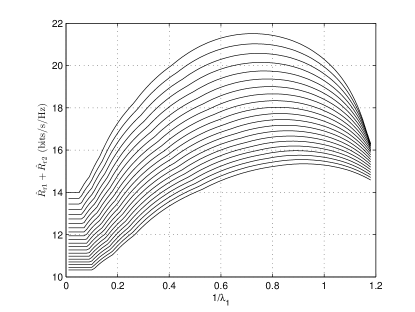
Figure 2: $\hat{R}_{\mathrm{r}1}+\hat{R}_{\mathrm{r}2}$ versus $1/\lambda_{1}$ under different $P^{\mathrm{max}}_{\mathrm{r}}/\sigma^{2}$.

Example 1: A demonstration of Lemma 2. It is assumed that the number of antennas at the relay $n_{\mathrm{r}}$ is 8 while source node 1 has $n_{1}=6$ antennas and source node 2 has $n_{2}=5$ antennas. Each curve in Fig. 2 shows the sum-rate $\hat{R}_{\mathrm{r}1}+\hat{R}_{\mathrm{r}2}$ versus the water-level $1/\lambda_{1}$ for a given ratio of $P^{\mathrm{max}}_{\mathrm{r}}$ over $\sigma^{2}$. In each curve, for each given $1/\lambda_{1}$, the relay consumes all the remaining power to maximize $1/\lambda_{2}$. Therefore, the power consumption of the relay is fixed and equals $P^{\mathrm{max}}_{\mathrm{r}}$. For each curve, $\sigma^{2}$ is different. The curve at the bottom corresponds to the ratio $P^{\mathrm{max}}_{\mathrm{r}}/\sigma^{2}$ equal to $4~{}\text{dB}$. For each time, when the ratio of $P^{\mathrm{max}}_{\mathrm{r}}$ over $\sigma^{2}$ increases, a new curve of $\hat{R}_{\mathrm{r}1}+\hat{R}_{\mathrm{r}2}$ versus $1/\lambda_{1}$, which lies above the previous curve, is plotted. The curve at the top corresponds to the ratio $P^{\mathrm{max}}_{\mathrm{r}}/\sigma^{2}$ equal to $7~{}\text{dB}$. It can be seen from Fig. 2 that the sum-rate $\hat{R}_{\mathrm{r}1}+\hat{R}_{\mathrm{r}2}$ is a nonconvex function of $1/\lambda_{1}$. However, $\hat{R}_{\mathrm{r}1}+\hat{R}_{\mathrm{r}2}$ is non-decreasing in the interval from the minimum $1/\lambda_{1}$ to the sum-rate maximizing $1/\lambda_{1}$ and non-increasing from the sum-rate maximizing $1/\lambda_{1}$ to the maximum $1/\lambda_{1}$. Note that $1/\lambda_{1}=1/\lambda_{2}=1/\lambda^{0}$ when the BC phase sum-rate is maximized. As a result, it can be seen that increasing $\max\{1/\lambda_{1},1/\lambda_{2}\}$ and decreasing $\min\{1/\lambda_{1},1/\lambda_{2}\}$ while fixing the total power consumption leads to a smaller BC phase sum-rate for any given $\{1/\lambda_{1},1/\lambda_{2}\}$. Therefore, Fig. 2 verifies the result presented in Lemma 2.

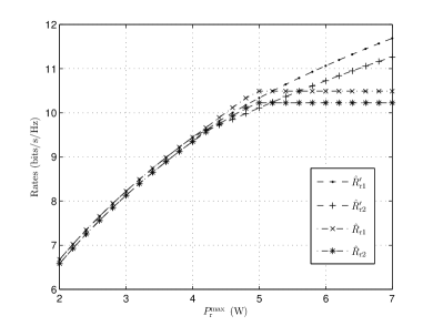
(a) $\hat{R}_{\mathrm{r}i}$ in the optimal solution of the sum-rate maximizing problems with and without minimizing power consumption, respectively, versus $P_{\rm r}^{\rm max}$

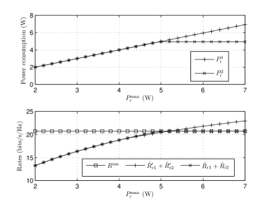
(b) Relay power consumption, $R^{\rm ma}(\mathbf{D}^{0})$ and $\sum\limits_{i}\hat{R}_{\mathrm{r}i}$ in the optimal solution of the sum-rate maximizing problems with and without minimizing power consumption, respectively, versus $P_{\rm r}^{\rm max}$

Figure 3: Illustration of relay optimization.

Example 2: The relay optimization problem. Fig. 3a compares the BC phase rates at optimality of the relay optimization problem, which considers power consumption minimization, with the BC phase rates at optimality of the problem (11), which does not minimize the power consumption, under different $P_{\mathrm{r}}^{\mathrm{max}}$. One channel realization is shown. The specific setup for this simulation is as follows. The number of antennas $n_{1},n_{2}$, and $n_{\mathrm{r}}$ are set to be $6,5$ and $8$, respectively. The power limits for the source nodes are set to be $P_{1}^{\mathrm{max}}=P_{2}^{\mathrm{max}}=3~{}\text{W}$. The noise variance is normalized so that $\sigma^{2}=1$. The MA phase rates for this channel realization are 20.7 for $R^{\mathrm{ma}}(\mathbf{D}^{0})$, 11.2 for $\bar{R}_{1\mathrm{r}}(\mathbf{D}_{1}^{0})$, and 11.0 for $\bar{R}_{2\mathrm{r}}(\mathbf{D}_{2}^{0})$. In Fig. 3a, $\hat{R}_{\mathrm{r}i}^{\prime}$ represents $\hat{R}_{\mathrm{r}i}(\mathbf{B}_{i}^{\prime})$, where $\mathbf{B}_{i}^{\prime}$’s, $\forall i$ are the optimal solution (obtained using CVX [23]) to the problem (11) which does not minimize the power consumption, and $\hat{R}_{\mathrm{r}i}$ represents $\hat{R}_{\mathrm{r}i}(\mathbf{B}_{i})$, where $\mathbf{B}_{i}$’s, $\forall i$ are the optimal solution to the relay optimization problem considering power consumption minimization obtained using the algorithm in Table I. It can be seen from Fig. 3a that $\hat{R}_{\mathrm{r}i}^{\prime}=\hat{R}_{\mathrm{r}i}$ when $P_{\mathrm{r}}^{\mathrm{max}}$ is small. The reason is that $\hat{R}_{\mathrm{r}i}^{\prime}$ is small when $P_{\mathrm{r}}^{\rm max}$ is below certain threshold. As a result, the constraints in $\eqref{e:RlconsPM}$ are always satisfied and the solutions to the problem (11) and the relay optimization problem are the same. As $P_{\mathrm{r}}^{\rm max}$ increases, $R^{\rm tw}(\mathbf{B},\mathbf{D}^{0})$ becomes larger and is finally bounded by $R^{\rm ma}(\mathbf{D}^{0})$, while the relay power consumption is not necessarily minimized in the solution of the problem (11) which does not consider power consumption minimization. This can be seen from the first subplot of Fig. 3b, which shows that the power consumption in the solution derived using the proposed algorithm, denoted as $P_{\mathrm{r}}^{2}$, saturates when $P_{\mathrm{r}}^{\mathrm{max}}\geq 4.9~{}\text{{\color[rgb]{0,0,0}W}}$, while the power consumption in the solution to the problem (11) which does not consider power consumption minimization, denoted as $P_{\mathrm{r}}^{1}$, keeps increasing. As a result, as can be seen from the second subplot of Fig. 3b, $\sum\limits_{i}\hat{R}_{\mathrm{r}i}$ never exceeds $R^{\mathrm{ma}}(\mathbf{D}^{0})$, while $\sum\limits_{i}\hat{R}_{\mathrm{r}i}^{\prime}$ grows beyond $R^{\mathrm{ma}}(\mathbf{D}^{0})$ when $R^{\rm tw}(\mathbf{B},\mathbf{D}^{0})$ is bounded by $R^{\mathrm{ma}}(\mathbf{D}^{0})$. Meanwhile, it can also be seen from the second subplot of Fig. 3b that the maximum sum-rates $R^{\rm tw}(\mathbf{B},\mathbf{D}^{0})$ for the two compared solutions are the same, both of which equal to $\sum\limits_{i}\hat{R}_{\mathrm{r}i}^{\prime}=\sum\limits_{i}\hat{R}_{\mathrm{r}i}$ when $\sum\limits\hat{R}_{\mathrm{r}i}^{\prime}\leq R^{\mathrm{ma}}(\mathbf{D}^{0})$ and equal to $R^{\mathrm{ma}}(\mathbf{D}^{0})$ when $\sum\limits\hat{R}_{\mathrm{r}i}^{\prime}>R^{\mathrm{ma}}(\mathbf{D}^{0})$. Thus, this example demonstrates that the proposed algorithm in Table I achieves maximum sum-rate in the scenario of relay optimization with minimum power consumption.

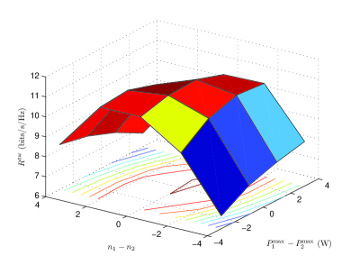
(a) Sum-rate at optimality.

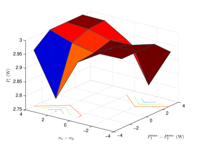
(b) Relay power consumption at optimality.

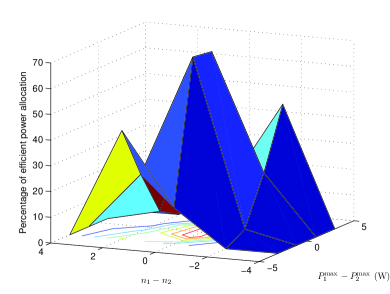
(c) Percentage of efficient power allocation at optimality.

Figure 4: Effect of asymmetry: the average sum-rate, average relay power consumption, and percentage of efficient power allocation at optimality of relay optimization versus the difference between number of antennas and the difference between power limits at the source nodes in 1000 channel realizations.

Example 3: The effect of asymmetry. The specific setup for this example is as follows. The noise variance is normalized so that $\sigma^{2}=1$. The number of antennas at the relay, i.e., $n_{\mathrm{r}}$, is set to be $6$. The power limit of the relay, i.e., $P^{\rm max}_{\mathrm{r}}$ is set to be 3 W. The total number of antennas at both source nodes is fixed such that $n_{1}+n_{2}=6$. The total available power at both source nodes is also fixed such that $P^{\rm max}_{1}+P^{\rm max}_{2}=5~{}\text{{\color[rgb]{0,0,0}W}}$. Given the above total number of antennas and total available power at the source nodes, the relay optimization problem is solved for different $n_{1}$, $n_{2}$, $P^{\rm max}_{1}$, and $P^{\rm max}_{2}$ for 1000 channel realizations. The resulting average sum-rate and average power consumption of the relay, and the percentage of efficient power allocation at optimality are plotted in Figs. 4a, 4b and 4c, respectively, versus the difference between the number of antennas and the difference between the power limits at the source nodes. From Fig. 4a, it can be seen that the sum-rate at optimality of the relay optimization is the largest when there is no asymmetry in the number of antennas at the source nodes and no asymmetry or only small asymmetry in the power limits of the source nodes. As the asymmetry becomes larger in either number of antennas or power limits, the sum-rate at optimality of the relay optimization decreases. Therefore, it can be seen from this figure that the asymmetry in the above aspects leads to smaller sum-rate at optimality of the considered relay optimization problem. Relating Figs. 4b and 4c to Fig. 4a, two more observations can be made. First, the relay does not necessarily use all the available power for sum-rate maximization in the relay optimization scenario. Second, the asymmetry in number of antennas and power limits leads to low power allocation efficiency. It can be seen from Fig. 4b that when one of $P_{1}^{\rm max}-P_{2}^{\rm max}$ and $n_{1}-n_{2}$ is positive while the other is negative, the relay uses a part of its available power. However, the achieved sum-rate is smaller compared to the sum-rate in the case when $P_{1}^{\rm max}-P_{2}^{\rm max}=0$ and $n_{1}-n_{2}=0$ (see Fig. 4a). In this situation, since the average power consumption and the average sum-rate are both low, the percentage of efficient power allocation is larger than 0 but less than the percentage when $P_{1}^{\rm max}-P_{2}^{\rm max}=0$ and $n_{1}-n_{2}=0$, as can be seen from Fig. 4c. When $P_{1}^{\rm max}-P_{2}^{\rm max}$ and $n_{1}-n_{2}$ are both positive or both negative, the relay uses more power than the power used in the case when $P_{1}^{\rm max}-P_{2}^{\rm max}=0$ and $n_{1}-n_{2}=0$ while the achieved sum-rate is smaller than that in the latter case. In this situation, since the average power consumption is high while the average sum-rate is low, the percentage of efficient power allocation is very low, if not zero, as can be seen from Fig. 4c. The above facts become more obvious when the asymmetry becomes larger. Therefore, it can be seen from Figs. 4b and 4c that the asymmetry on the power limits and the number of antennas can lead to low power allocation efficiency.

V Conclusion

In Part I of this two-part paper, we have solved the problem of sum-rate maximization with minimum power consumption for MIMO DF TWR in the scenario of relay optimization. For finding the optimal solution, we have proved the sufficient and necessary optimality condition for power allocation. Based on this condition, we have proposed an algorithm to find the optimal solution. The proposed algorithm allows the relay to obtain its optimal power allocation in several steps. We have shown that, as a trade-off for low complexity, there can be waste of power at the source nodes in the relay optimization scenario because of the lack of coordination. We have also shown that the asymmetry in the number of antennas and power limits at the source nodes can result in the degradation of the sum-rate performance and the power allocation efficiency in MIMO DF TWR. Next, in Part II of this two-part paper, we will investigate the scenario in which the relay and the source nodes jointly optimize their transmit strategies to achieve the network-level optimality of sum-rate maximization with minimum total power consumption for the MIMO DF TWR.

VI Appendix

VI-A Proof of Lemma 2

Lemma 2 is proved in two steps, i.e., Steps A and B. In Step A, we prove that $\sum\limits_{l}\hat{R}_{\mathrm{r}l}(\lambda_{l}^{\prime})$ can be increased by modifying the current power allocation on two specific subchannels. In Step B, we show that $\sum\limits_{l}\hat{R}_{\mathrm{r}l}(\lambda_{l}^{\prime})$ may be further increased.

Step A: $\sum\limits_{l}\hat{R}_{\mathrm{r}l}(\lambda_{l}^{\prime})$ can be increased. Given the fact that $\sum\limits_{l}\text{Tr}\{\mathbf{P}_{\mathrm{r}l}(\lambda_{l})\}=\sum\limits_{l}\text{Tr}\{\mathbf{P}_{\mathrm{r}l}(\lambda_{l}^{\prime})\}$, it can be shown that $1/\lambda_{i}^{\prime}>\min\limits_{k}\{1/\alpha_{i}(k)\}$ as long as $1/\lambda_{j}>\min\limits_{k}\{1/\alpha_{j}(k)\}$. As a result, there exist $k_{1}$ and $k_{2}$ such that $1/\lambda_{i}^{\prime}>1/\alpha_{i}(k_{1})$ and $1/\lambda_{j}>1/\alpha_{j}(k_{2})$. Define $f(p_{\mathrm{r}i}(k_{1}))=\log\big{(}1+\alpha_{i}(k_{1})p_{\mathrm{r}i}(k_{1})\big{)}+\log\big{(}1+\alpha_{j}(k_{2})p_{\mathrm{r}j}(k_{2})\big{)}$ where $p_{\mathrm{r}j}(k_{2})=p-p_{\mathrm{r}i}(k_{1})$ and $p$ is a positive constant. It can be seen that $f(p_{\mathrm{r}i}(k_{1}))$ is strictly concave in $p_{\mathrm{r}i}(k_{1})\in[0,p],\forall p>0$. Set $p=\big{(}1/\lambda_{j}^{{}^{\prime}}-1/\alpha_{j}(k_{2})\big{)}^{+}+1/\lambda_{i}^{\prime}-1/\alpha_{i}(k_{1})$. The optimal allocation of the power $p$ on $\alpha_{i}(k_{1})$ and $\alpha_{j}(k_{2})$ that maximizes $f(p_{\mathrm{r}i}(k_{1}))$ is $p_{\mathrm{r}i}(k_{1})=\big{(}1/\lambda^{\rm opt}(p)-1/\alpha_{i}(k_{1})\big{)}^{+}$ and $p_{\mathrm{r}j}(k_{2})=\big{(}1/\lambda^{\rm opt}(p)-1/\alpha_{j}(k_{2})\big{)}^{+}$ where $\lambda^{\rm opt}(p)$ is a function of $p$ and $1/\lambda^{\rm opt}(p)$ is the optimal water level. It can be shown that $1/\lambda^{\rm opt}(p)<1/\lambda_{i}^{\prime}$. There exist two cases, i.e., $1/\lambda^{\rm opt}(p)\leq 1/\lambda_{i}$ and $1/\lambda^{\rm opt}(p)>1/\lambda_{i}$. In the case when $1/\lambda^{\rm opt}(p)\leq 1/\lambda_{i}$, it follows that $\big{(}1/\lambda^{\rm opt}(p)-1/\alpha_{i}(k_{1})\big{)}^{+}\leq\big{(}1/\lambda_{i}-1/\alpha_{i}(k_{1}))^{+}<1/\lambda_{i}^{\prime}-1/\alpha_{i}(k_{1})$. The power allocation on $k_{1}$ and $k_{2}$ using $\lambda_{i}^{\prime}$ and $\lambda_{j}^{\prime}$ is

$$p_{\mathrm{r}i}(k_{1})=\bigg{(}\frac{1}{\lambda_{i}^{\prime}}-\frac{1}{\alpha_{i}(k_{1})}\bigg{)}^{+}$$ (24a)

$$p_{\mathrm{r}j}(k_{2})=\bigg{(}\frac{1}{\lambda_{j}^{\prime}}-\frac{1}{\alpha_{j}(k_{2})}\bigg{)}^{+}.$$ (24b)

Since $f(p_{\mathrm{r}i}(k_{1}))$ is strictly concave as mentioned above, it can be seen that the power allocation

$$p_{\mathrm{r}i}(k_{1}) =\bigg{(}\frac{1}{\lambda_{i}}-\frac{1}{\alpha_{i}(k_{1})}\bigg{)}^{+}$$ (25a)

$$p_{\mathrm{r}j}(k_{2}) =\bigg{(}\frac{1}{\lambda_{j}^{\prime}}-\frac{1}{\alpha_{j}(k_{2})}\bigg{)}^{+}$$

$$\;\;\;+\frac{1}{\lambda_{i}^{\prime}}-\frac{1}{\alpha_{i}(k_{1})}-\bigg{(}\frac{1}{\lambda_{i}}-\frac{1}{\alpha_{i}(k_{1})}\bigg{)}^{+}$$ (25b)

which reduces $p_{\mathrm{r}i}(k_{1})$ and increases $p_{\mathrm{r}j}(k_{2})$, both by ${1}/{\lambda_{i}^{\prime}}-{1}/{\alpha_{i}(k_{1})}-\big{(}{1}/{\lambda_{i}}-{1}/{\alpha_{i}(k_{1})}\big{)}^{+}$, yields higher $f(p_{\mathrm{r}i}(k_{1}))$ than the power allocation in (24).

Therefore, the sum-rate $\sum\limits_{l}\sum\limits_{k}\log\big{(}1+\alpha_{l}(k)p_{\mathrm{r}l}(k)\big{)}$ achieved using (25) and

$$p_{\mathrm{r}i}(k)=\bigg{(}\frac{1}{\lambda_{i}^{\prime}}-\frac{1}{\alpha_{i}(k)}\bigg{)}^{+},\forall k\in\mathcal{I}_{i}\setminus\{k_{1}\}$$ (26a)

$$p_{\mathrm{r}j}(k)=\bigg{(}\frac{1}{\lambda_{j}^{\prime}}-\frac{1}{\alpha_{j}(k)}\bigg{)}^{+},\forall k\in\mathcal{I}_{j}\setminus\{k_{2}\}$$ (26b)

is larger than $\sum\limits_{l}\hat{R}_{\mathrm{r}l}(\lambda_{l}^{\prime})$. This is the first step of increasing sum-rate. Moreover, it can be seen that there exists $\tilde{\lambda}_{j}$ such that

$$\qquad\qquad\qquad\qquad\frac{1}{\lambda_{j}^{\prime}}<\frac{1}{\tilde{\lambda}_{j}}<\frac{1}{\lambda_{j}}$$ (27a)

$$\text{Tr}\{\mathbf{P}_{\mathrm{r}i}(\lambda_{i}^{\prime})\}-\bigg{(}\frac{1}{\lambda_{i}^{\prime}}-\frac{1}{\alpha_{i}(k_{1})}\bigg{)}^{+}+\bigg{(}\frac{1}{\lambda_{i}}-\frac{1}{\alpha_{i}(k_{1})}\bigg{)}^{+}$$

$$\qquad\qquad+\text{Tr}\{\mathbf{P}_{\mathrm{r}j}(\tilde{\lambda}_{j})\}=\sum\limits_{l}\text{Tr}\{\mathbf{P}_{\mathrm{r}l}(\lambda_{l}^{\prime})\}$$ (27b)

and the power allocation

$$p_{\mathrm{r}i}(k_{1})=\bigg{(}\frac{1}{\lambda_{i}}-\frac{1}{\alpha_{i}(k)}\bigg{)}^{+}$$ (28a)

$$p_{\mathrm{r}i}(k)=\bigg{(}\frac{1}{\lambda_{i}^{\prime}}-\frac{1}{\alpha_{i}(k)}\bigg{)}^{+},\forall k\in\mathcal{I}_{i}\setminus\{k_{1}\}$$ (28b)

$$p_{\mathrm{r}j}(k)=\bigg{(}\frac{1}{\tilde{\lambda}_{j}}-\frac{1}{\alpha_{j}(k)}\bigg{)}^{+},\forall k\in\mathcal{I}_{j}$$ (28c)

which spreads the power ${1}/{\lambda_{i}^{\prime}}-{1}/{\alpha_{i}(k_{1})}-\big{(}{1}/{\lambda_{i}}-{1}/{\alpha_{i}(k_{1})}\big{)}^{+}$ over ${\alpha_{j}(k)}$’s, $\forall k\in\mathcal{I}_{j}$, achieves even higher sum-rate than that achieved by the power allocation specified by (25) and (26). This is the second step of increasing the sum-rate.

For the second case in which $1/\lambda_{i}<1/\lambda^{\rm opt}(p)<1/\lambda_{i}^{\prime}$, the following process is adopted. Similar to the two steps of increasing the sum-rate in the first case, the sum-rate $\sum\limits_{l}\sum\limits_{k}\log\big{(}1+\alpha_{l}(k)p_{\mathrm{r}l}(k)\big{)}$ increases after each of the following two adjustments of power allocation. First, reduce $p_{\mathrm{r}i}(k_{1})$ from $1/\lambda_{i}^{\prime}-1/\alpha_{i}(k_{1})$ to $\big{(}1/\lambda^{\rm opt}(p)-1/\alpha_{i}(k_{1})\big{)}^{+}$. Then, spread the reduced power ${1}/{\lambda_{i}^{\prime}}-{1}/{\alpha_{i}(k_{1})}-\big{(}{1}/{\lambda^{\rm opt}(p)}-{1}/{\alpha_{i}(k_{1})}\big{)}^{+}$ over ${\alpha_{j}(k)}$’s $,k\in\mathcal{I}_{j}$ by finding and using $1/\tilde{\lambda}_{j}^{\prime}$ which satisfies

$$\text{Tr}\{\mathbf{P}_{\mathrm{r}i}(\lambda_{i}^{\prime})\}-\bigg{(}\frac{1}{\lambda_{i}^{\prime}}-\frac{1}{\alpha_{i}(k_{1})}\bigg{)}^{+}+\bigg{(}\frac{1}{\lambda^{\rm opt}(p)}-\frac{1}{\alpha_{i}(k_{1})}\bigg{)}^{+}$$

$$+\text{Tr}\{\mathbf{P}_{\mathrm{r}j}(\tilde{\lambda}_{j}^{\prime})\}=\sum\limits_{l}\text{Tr}\{\mathbf{P}_{\mathrm{r}l}(\lambda_{l}^{\prime})\}.$$ (29)

After the adjustments, it is straightforward to see that the total power allocated on $k_{1}$ and $k_{2}$ is reduced from $p=\big{(}1/\lambda_{j}^{\prime}-1/\alpha_{j}(k_{2})\big{)}^{+}+1/\lambda_{i}^{\prime}-1/\alpha_{i}(k_{1})$ to $\bar{p}=\big{(}1/\tilde{\lambda}_{j}^{\prime}-1/\alpha_{j}(k_{2})\big{)}^{+}+\big{(}1/\lambda^{\rm opt}(p)-1/\alpha_{i}(k_{1})\big{)}^{+}$. In consequence, there exists a new optimal water level $1/\lambda^{\rm opt}(\bar{p})$ based on which the optimal allocation of the power $\bar{p}$, i.e., $p_{\mathrm{r}i}(k_{1})=\big{(}1/\lambda^{\rm opt}(\bar{p})-1/\alpha_{i}(k_{1})\big{)}^{+}$ and $p_{\mathrm{r}j}(k_{2})=1/\lambda^{\rm opt}(\bar{p})-1/\alpha_{j}(k_{2})$, maximizes $f(p_{\mathrm{r}i}(k_{1}))$ when $p$ in $f(p_{\mathrm{r}i}(k_{1}))$ is substituted by $\bar{p}$. Since $\bar{p}<p$, it can be seen that $1/\lambda^{\rm opt}(\bar{p})<1/\lambda^{\rm opt}(p)$. Update $p$ and $1/\lambda^{\rm opt}(p)$ so that $p=\bar{p}$ and $1/\lambda^{\rm opt}(p)=1/\lambda^{\rm opt}(\bar{p})$. Then the above process of reducing $p_{\mathrm{r}i}(k_{1})$ to $\big{(}1/\lambda^{\rm opt}(p)-1/\alpha_{i}(k_{1})\big{)}^{+}$, finding the new $1/\tilde{\lambda}_{j}^{\prime}$ and the new $1/\lambda^{\rm opt}(p)$ can be repeated until a). $1/\lambda^{\rm opt}(p)\leq 1/\lambda_{i}$ or until b). $1/\lambda^{\rm opt}(p)\leq 1/\alpha_{i}(k_{1})$. The former matches the condition for the first case discussed in the previous paragraph and therefore can be dealt with in the same way as in the first case, which leads to (28). The latter implies that $1/\lambda_{i}<1/\lambda^{\rm opt}(p)\leq 1/\alpha_{i}(k_{1})$, in which case the power allocation can also be equivalently written as (28). Note that during this process the sum-rate $\sum\limits_{l}\sum\limits_{k}\log\big{(}1+\alpha_{l}(k)p_{\mathrm{r}l}(k)\big{)}$ increases. Therefore, summarizing the above two cases of $1/\lambda^{\rm opt}(p)\leq 1/\lambda_{i}$ and $1/\lambda^{\rm opt}(p)>1/\lambda_{i}$, it is proved that the sum-rate can be increased by reducing $p_{\mathrm{r}i}(k_{1})$ from $1/\lambda_{i}^{\prime}-1/\alpha_{i}(k_{1})$ to $\big{(}1/\lambda_{i}-1/\alpha_{i}(k_{1})\big{)}^{+}$ and using the power allocation in (28).

Step B: $\sum\limits_{l}\hat{R}_{\mathrm{r}l}(\lambda_{l}^{\prime})$ may be further increased. Keep the above selected $k_{2}$ unchanged. As long as there exists $k$ such that $p_{\mathrm{r}i}(k)=\big{(}1/\lambda_{i}^{\prime}-1/\alpha_{i}(k_{1})\big{)}^{+}$ and $p_{\mathrm{r}i}(k)>0$, this $k$ can be selected as $k_{1}$ and the procedure of reducing $p_{\mathrm{r}i}(k_{1})$ from $1/\lambda_{i}^{\prime}-1/\alpha_{i}(k_{1})$ to $\big{(}1/\lambda_{i}-1/\alpha_{i}(k_{1})\big{)}^{+}$ and spreading the reduced power over ${\alpha_{j}(k)}$’s, $\forall k\in\mathcal{I}_{j}$ as specified in (28) can be performed. This process can be repeated until $p_{\mathrm{r}i}(k)=\big{(}1/\lambda_{i}-1/\alpha_{i}(k)\big{)}^{+},\forall k\in\{q\in\mathcal{I}_{i}|\big{(}1/\lambda_{i}^{\prime}-1/\alpha_{i}(q)\big{)}^{+}>0\}$ and $p_{\mathrm{r}i}(k)=0,\forall k\in\{q\in\mathcal{I}_{i}|\big{(}1/\lambda_{i}^{\prime}-1/\alpha_{i}(q)\big{)}^{+}=0\}$. Note that the sum-rate $\sum\limits_{l}\sum\limits_{k}\log\big{(}1+\alpha_{l}(k)p_{\mathrm{r}l}(k)\big{)}$ increases in the above process for every qualifying $k_{1}$. The resulting power allocation on $\alpha_{i}(k)$’s, $\forall k\in\mathcal{I}_{i}$ is equivalent to $p_{\mathrm{r}i}(k)=\big{(}1/\lambda_{i}-1/\alpha_{i}(k)\big{)}^{+},\forall k\in\mathcal{I}_{i}$ since $\big{(}1/\lambda_{i}-1/\alpha_{i}(k)\big{)}^{+}=0$ if $\big{(}1/\lambda_{i}^{\prime}-1/\alpha_{i}(k)\big{)}^{+}=0$. From the procedure described in the previous paragraphes, the resulting power allocation on $\alpha_{j}(k)$’s, $\forall k\in\mathcal{I}_{j}$ is $p_{\mathrm{r}j}(k)=\big{(}1/\tilde{\lambda}_{j}-1/\alpha_{j}(k)\big{)}^{+},\forall k$. According to the power constraint $\sum\limits_{l}\text{Tr}\{\mathbf{P}_{\mathrm{r}l}(\lambda_{l})\}=\sum\limits_{l}\text{Tr}\{\mathbf{P}_{\mathrm{r}l}(\lambda_{l}^{\prime})\}$ and the fact that the total power consumption is fixed at all time, it can be seen that $1/\tilde{\lambda}_{j}=1/\lambda_{j}$.

Summarizing the above two steps, Lemma 2 is proved. $\blacksquare$

VI-B Proof of Lemma 3

Given that $\lambda_{i}^{\prime}\leq\lambda_{j}$, we have $\lambda_{i}<\lambda_{i}^{\prime}\leq\lambda_{j}<\lambda_{j}^{\prime}$. According to Lemma 2, there exists $\tilde{\lambda}_{i}<\lambda_{i}^{\prime}$ such that

$$\text{Tr}\{\mathbf{P}_{\mathrm{r}i}(\lambda_{i}^{\prime})\}+\text{Tr}\{\mathbf{P}_{\mathrm{r}j}(\lambda_{j})\}\qquad\qquad$$

$$\qquad\quad\quad\;\,=\text{Tr}\{\mathbf{P}_{\mathrm{r}i}(\tilde{\lambda}_{i})\}+\text{Tr}\{\mathbf{P}_{\mathrm{r}j}(\lambda_{j}^{\prime})\}$$ (30)

and

$$\hat{R}_{\mathrm{r}i}(\lambda_{i}^{\prime})+\hat{R}_{\mathrm{r}j}(\lambda_{j})>\hat{R}_{\mathrm{r}i}(\tilde{\lambda}_{i})+\hat{R}_{\mathrm{r}j}(\lambda_{j}^{\prime}).$$ (31)

Therefore, given that

$$\hat{R}_{\mathrm{r}i}(\lambda_{i}^{\prime})+\hat{R}_{\mathrm{r}j}(\lambda_{j})=\hat{R}_{\mathrm{r}i}(\lambda_{i})+\hat{R}_{\mathrm{r}j}(\lambda_{j}^{\prime})$$ (32)

it is necessary that $\tilde{\lambda}_{i}>\lambda_{i}$. As a result, it leads to

$$\text{Tr}\{\mathbf{P}_{\mathrm{r}i}(\lambda_{i}^{\prime})\}+\text{Tr}\{\mathbf{P}_{\mathrm{r}j}(\lambda_{j})\}\qquad\qquad$$

$$\qquad\quad\;\,<\text{Tr}\{\mathbf{P}_{\mathrm{r}i}(\lambda_{i})\}+\text{Tr}\{\mathbf{P}_{\mathrm{r}j}(\lambda_{j}^{\prime})\}.$$ (33)

Lemma 3 is thereby proved. $\blacksquare$

VI-C Proof of Theorem 1

First we prove that the optimal water-levels must satisfy condition (17a). It can be seen that the maximum $R^{\rm tw}(\mathbf{B},\mathbf{D})$ is achieved with minimum power consumption using $\lambda_{1}=\lambda_{2}=\max\{\lambda^{0},\mu_{\mathrm{ma}}^{0}\}$ when $\min\{1/\mu_{1}^{0},1/\mu_{2}^{0}\}\geq 1/\mu_{\mathrm{ma}}$ at the optimality. Therefore, it is necessary that $\min\{1/\mu_{1}^{0},1/\mu_{2}^{0}\}<1/\mu_{\rm ma}^{0}$ given that $\lambda_{1}\neq\lambda_{2}$ at optimality. Let us consider the case when $\min\{1/\lambda_{1},1/\lambda_{2}\}=1/\lambda_{1}<1/\lambda_{2}$ at optimality. According to the constraint (14a), we have that $1/\lambda_{1}\leq 1/\mu_{2}^{0}$ at optimality. Similarly, it can be seen that $1/\lambda_{2}\leq 1/\mu_{1}^{0}$ at optimality. Since $1/\lambda_{1}<1/\lambda_{2}$, it leads to the result that $1/\lambda_{1}\leq 1/\mu_{2}^{0}<1/\mu_{1}^{0}$ at optimality. Assuming that $\min\{1/\mu_{1}^{0},1/\mu_{2}^{0}\}\neq 1/\lambda_{1}$ at optimality when $\lambda_{1}\neq\lambda_{2}$, it infers that $1/\lambda_{1}<1/\mu_{2}^{0}<1/\lambda_{2}$. However, it can be seen that the power allocation using $1/\lambda_{1}<1/\mu_{2}^{0}<1/\lambda_{2}$ does not provide the maximum achievable $R^{\rm tw}(\mathbf{B},\mathbf{D})$ according to Lemma 2. Consequently, the resulting power allocation is not optimal. It contradicts the assumption that $\min\{1/\mu_{1}^{0},1/\mu_{2}^{0}\}\neq 1/\lambda_{1}$ at optimality. Thus, the above assumption is invalid and it is necessary that $\min\{1/\mu_{1}^{0},1/\mu_{2}^{0}\}=1/\lambda_{1}$ at optimality when $\lambda_{1}\neq\lambda_{2}$. Similarly, it can be proved that $\min\{1/\mu_{1}^{0},1/\mu_{2}^{0}\}=1/\lambda_{2}$ at optimality when $\lambda_{1}\neq\lambda_{2}$ for the case when $\min\{1/\lambda_{1},1/\lambda_{2}\}=1/\lambda_{2}<1/\lambda_{1}$. Therefore, it always holds true that $\min\{\frac{1}{\lambda_{1}},\frac{1}{\lambda_{2}}\}=\min\{\frac{1}{\mu_{1}^{0}},\frac{1}{\mu_{2}^{0}}\}$ if $\lambda_{1}\neq\lambda_{2}$.

Next we prove that the optimal water-levels must satisfy condition (17b). It is straightforward to see that $1/\lambda_{1}=1/\lambda_{2}\leq 1/\lambda^{0}$. Moreover, according to the constraints (14a) and (14b), it is not difficult to see that $1/\lambda_{1}=1/\lambda_{2}\leq\min\{1/\mu_{1}^{0},1/\mu_{2}^{0},1/\mu_{\rm ma}^{0}\}$ when $1/\lambda_{1}=1/\lambda_{2}$ at optimality. Indeed, if $1/\lambda_{1}=1/\lambda_{2}>1/\mu_{\rm ma}^{0}$, then (14b) cannot be satisfied. If $1/\lambda_{1}=1/\lambda_{2}>\min\{1/\mu_{1}^{0},1/\mu_{2}^{0}\}$, then (14a) cannot be satisfied. Combining the above two facts, we have $1/\lambda_{1}=1/\lambda_{2}\leq\min\{1/\mu_{1}^{0},1/\mu_{2}^{0},1/\mu_{\rm ma}^{0},1/\lambda^{0}\}$ when $1/\lambda_{1}=1/\lambda_{2}$ at optimality. For the case that $\min\{1/\mu_{1}^{0},1/\mu_{2}^{0}\}\geq 1/\mu_{\rm ma}^{0}$, the above constraint can be written as $1/\lambda_{1}=1/\lambda_{2}\leq\min\{1/\mu_{\rm ma}^{0},1/\lambda^{0}\}$. For this case, it is straightforward to see that the achieved sum-rate is not maximized if $1/\lambda_{1}=1/\lambda_{2}<\min\{1/\mu_{\rm ma}^{0},1/\lambda^{0}\}$. Therefore, the optimal water-levels must satisfy condition (17b) when $\min\{1/\mu_{1}^{0},1/\mu_{2}^{0}\}\geq 1/\mu_{\rm ma}^{0}$ given that $1/\lambda_{1}=1/\lambda_{2}$. For the case when $\min\{1/\mu_{1}^{0},1/\mu_{2}^{0}\}<1/\mu_{\rm ma}^{0}$, it can be seen that $1/\lambda^{0}\leq\min\{1/\mu_{1}^{0},1/\mu_{2}^{0}\}$ given that $1/\lambda_{1}=1/\lambda_{2}$ at optimality. Otherwise, it can be shown that either of the following two results must occur. If $1/\lambda^{0}>\min\{1/\mu_{1}^{0},1/\mu_{2}^{0}\}$ and $1/\lambda_{1}=1/\lambda_{2}\leq\min\{1/\mu_{1}^{0},1/\mu_{2}^{0}\}$, then the sum-rate can be increased. If $1/\lambda^{0}>\min\{1/\mu_{1}^{0},1/\mu_{2}^{0}\}$ and $1/\lambda_{1}=1/\lambda_{2}\geq\min\{1/\mu_{1}^{0},1/\mu_{2}^{0}\}$, then the constraint (14a) cannot be satisfied. Therefore, given that $1/\lambda^{0}\leq\min\{1/\mu_{1}^{0},1/\mu_{2}^{0}\}$ for the case when $\min\{1/\mu_{1}^{0},1/\mu_{2}^{0}\}<1/\mu_{\rm ma}^{0}$ and $1/\lambda_{1}=1/\lambda_{2}$ at optimality, we have $1/\lambda^{0}\leq\min\{1/\mu_{1}^{0},1/\mu_{2}^{0}\}<1/\mu_{\rm ma}^{0}$. Consequently, the constraint $1/\lambda_{1}=1/\lambda_{2}\leq\min\{1/\mu_{1}^{0},1/\mu_{2}^{0},1/\mu_{\rm ma}^{0},1/\lambda^{0}\}$ can be rewritten as $1/\lambda_{1}=1/\lambda_{2}\leq 1/\lambda^{0}=\min\{1/\mu_{\rm ma}^{0},1/\lambda^{0}\}$. It is straightforward to see for this case that $1/\lambda_{1}=1/\lambda_{2}<1/\lambda^{0}$ does not maximize the sum-rate. Therefore, it can also be concluded that $1/\lambda_{1}=1/\lambda_{2}=1/\lambda^{0}=\min\{1/\mu_{\rm ma}^{0},1/\lambda^{0}\}$ when $\min\{1/\mu_{1}^{0},1/\mu_{2}^{0}\}<1/\mu_{\rm ma}^{0}$. Combining the above two cases of $\min\{1/\mu_{1}^{0},1/\mu_{2}^{0}\}\geq 1/\mu_{\rm ma}^{0}$ and $\min\{1/\mu_{1}^{0},1/\mu_{2}^{0}\}<1/\mu_{\rm ma}^{0}$, it can be seen that the optimal water-levels always satisfy condition (17b) given that $1/\lambda_{1}=1/\lambda_{2}$.

The above two parts complete the proof of Theorem 1. $\hfill\blacksquare$

VI-D Proof of Theorem 2

The necessity of the constraints (14a) and (14b) is straightforward. It can be seen that the power consumption can be reduced without reducing the sum-rate $R^{\mathrm{tw}}(\mathbf{B},\mathbf{D})$ when these constraints are not satisfied. The necessity of the constraints (17a) and (17b) is proved in Theorem 1 in Section VI-C. Therefore, we next prove the sufficiency of the constraints (14a), (14b), (17a), and (17b).

We use proof by contradiction. Assume that the above constrains are not sufficient to determine the optimal $\{\lambda_{1},\lambda_{2}\}$ with minimum power consumption among all $\{\lambda_{1},\lambda_{2}\}$’s that maximize the sum-rate $R^{\rm tw}(\mathbf{B},\mathbf{D})$. Then there exists $\{\lambda_{1}^{\dagger},\lambda_{2}^{\dagger}\}$ satisfying (14) and (17a)-(17b) that maximizes the sum-rate and does not minimize the power consumption. Consequently, at least one of $1/\lambda_{1}^{\dagger}$ and $1/\lambda_{2}^{\dagger}$ can be reduced without reducing $R^{\rm tw}(\mathbf{B},\mathbf{D})$. We consider the following two cases. The first case is when $\lambda_{1}^{\dagger}\neq\lambda_{2}^{\dagger}$ while the second case is when $\lambda_{1}^{\dagger}=\lambda_{2}^{\dagger}$. In the first case, $\{\lambda_{1}^{\dagger},\lambda_{2}^{\dagger}\}$ satisfies (17a) and it is straightforward to see that reducing $\min\{1/\lambda_{1}^{\dagger},1/\lambda_{2}^{\dagger}\}$ is not optimal according to Lemma 3. Reducing $\max\{1/\lambda_{1}^{\dagger},1/\lambda_{2}^{\dagger}\}$, on the other hand, necessarily leads to the decrease of $R^{\rm tw}(\mathbf{B},\mathbf{D})$ given that (14b) is satisfied. Therefore, reducing either of $1/\lambda_{1}^{\dagger}$ and $1/\lambda_{2}^{\dagger}$ results in the decrease of the sum-rate, which contradicts the previous assumption. In the second case, $\{\lambda_{1}^{\dagger},\lambda_{2}^{\dagger}\}$ satisfies (17b). According to Theorem 2, it is necessary that $1/\lambda_{1}^{\dagger}=1/\lambda_{2}^{\dagger}=\min\{1/\mu_{\rm ma}^{0},1/\lambda^{0}\}$. From Lemma 2, it can be seen that it is not optimal to reduce only one of $1/\lambda_{1}^{\dagger}$ and $1/\lambda_{2}^{\dagger}$. Reducing both of $1/\lambda_{1}^{\dagger}$ and $1/\lambda_{2}^{\dagger}$, on the other hand, necessarily leads to the decrease of $R^{\rm tw}(\mathbf{B},\mathbf{D})$ given that (14b) is satisfied. Therefore, it is impossible that there exists $\{\lambda_{1}^{\dagger},\lambda_{2}^{\dagger}\}$ with $\lambda_{1}^{\dagger}=\lambda_{2}^{\dagger}$, satisfying (14) and (17b), that maximizes the sum-rate while the resulting power consumption can be reduced. Combining the above two cases, it can be seen that the power consumption cannot be reduced given that the $\{\lambda_{1}^{\dagger},\lambda_{2}^{\dagger}\}$ maximizes the sum-rate subject to the relay power limit and satisfies (14) and (17a)-(17b). This contradicts the assumption that the above constrains are not sufficient to determine the optimal $\{\lambda_{1},\lambda_{2}\}$ with minimum power consumption among all $\{\lambda_{1},\lambda_{2}\}$’s that maximize $R^{\rm tw}(\mathbf{B},\mathbf{D})$. This completes the proof for Theorem 2. $\blacksquare$

VI-E Proof of Theorem 3

The optimality of the pair $\{\lambda_{1},\lambda_{2}\}$ obtained using the algorithm in Table I is proved in three steps: A) Steps 2-5 of the algorithm in Table I find $\{\lambda_{1},\lambda_{2}\}$ that maximizes $R^{\mathrm{bc}}(\mathbf{B},\mathbf{D}^{0})$ with minimum power consumption subject to the constraint in (11) and the constraint (14a). B) The pair $\{\lambda_{1},\lambda_{2}\}$ obtained from Steps 2-5 of the algorithm in Table I needs to be modified to maximize the objective function in (11) with minimum power consumption. Step 6 of the algorithm in Table I deals with two cases in which $\{\lambda_{1},\lambda_{2}\}$ obtained from the previous steps can be simply modified to obtain the optimal pair $\{\lambda_{1},\lambda_{2}\}$. C) Step 7 of the algorithm in Table I deals with the remaining case which is more complicated and finds the corresponding optimal pair $\{\lambda_{1},\lambda_{2}\}$ in this case. It is not difficult to see that the constraint in (11) is always satisfied in any step of the proposed algorithm. It can also be seen that Steps 1, 2 and 6 ensure that (17b) is satisfied if $\lambda_{1}=\lambda_{2}$ at the output of the algorithm while Steps 3 to 5 ensure that (17a) is satisfied if $\lambda_{1}\neq\lambda_{2}$ at the output. Therefore, in the following we only consider the constraints (14a) and (14b), which are equivalent to the constraints in (12).

A. Steps 2-5 find the pair $\{\lambda_{1},\lambda_{2}\}$ that maximizes $R(\mathbf{B},\mathbf{D}^{0})$ with minimum power consumption subject to the constraint (14a). Note that the maximum $R(\mathbf{B},\mathbf{D}^{0})$ with minimum power consumption is achieved by $\hat{R}_{\mathrm{r}1}(\lambda_{1})+\hat{R}_{\mathrm{r}2}(\lambda_{2})$ for some specific $\{\lambda_{1},\lambda_{2}\}$ if (14a) is satisfied. Therefore, it is equivalent to finding the $\{\lambda_{1},\lambda_{2}\}$ that maximizes $\hat{R}_{\mathrm{r}1}(\lambda_{1})+\hat{R}_{\mathrm{r}2}(\lambda_{2})$ subject to (14a). The initial power allocation in Step 1 of the algorithm in Table I using $1/\lambda_{1}=1/\lambda_{2}=1/\lambda^{0}$ maximizes $\hat{R}_{\mathrm{r}1}(\lambda_{1})+\hat{R}_{\mathrm{r}2}(\lambda_{2})$. Regarding the constraint (14a), the following cases are possible.

A-1. $\lambda_{i}\geq\mu_{j}^{0}$, $\forall i$. In this case, the constraint (14a) is satisfied and $\{\lambda^{0},\lambda^{0}\}$ is the desired $\{\lambda_{1},\lambda_{2}\}$.

A-2. $\lambda_{i}<\mu_{j}^{0}$ and $\lambda_{j}\geq\mu_{i}^{0}$. In this case, the constraint (14a) is not satisfied for $i$. The relay power consumption can be reduced without decreasing $R(\mathbf{B},\mathbf{D}^{0})$ by increasing $\lambda_{i}$ until $\lambda_{i}=\mu_{j}^{0}$. Then, $R(\mathbf{B},\mathbf{D}^{0})$ can be increased by decreasing $\lambda_{j}$ until the relay power limit is reached or until $\lambda_{j}=\mu_{i}^{0}$.

A-3. $\lambda_{i}<\mu_{j}^{0},\forall i$. In this case, it is straightforward to see that the pair $\{\lambda_{1},\lambda_{2}\}$ that maximizes $R(\mathbf{B},\mathbf{D}^{0})$ with minimum power consumption subject to the constraint (14a) satisfies $\lambda_{i}=\mu_{j}^{0},\forall i$.

The above three cases are determined in Step 2. Case A-1 is dealt with in Step 2 of the algorithm in Table I. Case A-2 is dealt with in Steps 3 and 4. Case A-3 is dealt with in Steps 3 and 5.

B. Steps 6 and 7 of the algorithm in Table I find the optimal pair $\{\lambda_{1},\lambda_{2}\}$ that maximizes the objective function in (11) with minimum power consumption. Since $R^{\rm ma}(\mathbf{D}^{0})<\bar{R}_{1\mathrm{r}}(\mathbf{D}_{1}^{0})+\bar{R}_{2\mathrm{r}}(\mathbf{D}_{2}^{0})$, it can be seen that $\lambda_{i},\forall i$ should either increase or remain the same in order to satisfy the constraint (14b) given that the constraint (14a) is satisfied. Therefore, the optimal power allocation can be derived by increasing $\lambda_{1}$ and/or $\lambda_{2}$, if necessary, based on the power allocation derived from Steps 1-5. Regarding the constraint (14b), the following cases are possible.

B-1. $\lambda_{i}\geq\mu_{\mathrm{ma}}^{0},\forall i$ or ($\lambda_{i}\geq\mu_{\mathrm{ma}}^{0}$, $\lambda_{j}<\mu_{\mathrm{ma}}^{0}$ and $\hat{R}_{\mathrm{r}1}(\lambda_{1})+\hat{R}_{\mathrm{r}2}(\lambda_{2})\leq R^{\rm ma}(\mathbf{D}^{0})$). In this case, the constraint (14b) is satisfied and the current $\{\lambda_{1},\lambda_{2}\}$ is optimal.

B-2. $\lambda_{i}<\mu_{\mathrm{ma}}^{0},\forall i$ and $\hat{R}_{\mathrm{r}1}(\lambda_{1})+\hat{R}_{\mathrm{r}2}(\lambda_{2})>R^{\rm ma}(\mathbf{D}^{0})$. In this case, it is not difficult to see that it is optimal to simply set $\lambda_{i}=\mu_{\mathrm{ma}}^{0},\forall i$.

B-3. $\lambda_{i}>\mu_{\mathrm{ma}}^{0}$, $\lambda_{j}<\mu_{\mathrm{ma}}^{0}$ and $\hat{R}_{\mathrm{r}1}(\lambda_{1})+\hat{R}_{\mathrm{r}2}(\lambda_{2})>R^{\rm ma}(\mathbf{D}^{0})$.

Cases B-1 and B-2 are simple and dealt with in Step 6 of the algorithm in Table I. It can be shown that in these two cases the constraints (14a) and (14b) are both necessary and sufficient for finding the optimal power allocation in terms of maximizing the sum-rate with minimum power consumption. Case B-3 is dealt with in Step 7. The optimal strategy in Case B-3, as in Step 7 of the algorithm in Table I, is to increase $\lambda_{j}$ while keeping $\lambda_{i}$ unchanged until $\hat{R}_{\mathrm{r}1}(\lambda_{1})+\hat{R}_{\mathrm{r}2}(\lambda_{2})=R^{\rm ma}(\mathbf{D}^{0})$. In order to prove that this strategy is optimal, the following three points are necessary and sufficient.

1. It is optimal to increase $\min\limits_{i}\{\lambda_{i}\}$.

2. $\lambda_{i}=\mu_{j}^{0}$ if $\lambda_{i}>\mu_{\mathrm{ma}}^{0}$ and $\lambda_{j}<\mu_{\mathrm{ma}}^{0}$.

3. At optimality, the increased $\lambda_{j}$, denoted as $\lambda_{j}^{\prime}$, satisfies $\lambda_{j}<\lambda_{j}^{\prime}<\mu_{\mathrm{ma}}^{0}$.

The first point states that it is optimal to increase $\lambda_{j}$ as long as $\lambda_{j}<\lambda_{i}$. The second point infers that it is not optimal to decrease $\lambda_{i}$. The third point infers that $\lambda_{j}^{\prime}$ is always larger than $\lambda_{i}$ and therefore it is not optimal to increase $\lambda_{i}$ at any time. The first point follows from Lemma 3. For the second point, assume that $\lambda_{i}>\mu_{j}^{0}$. It follows that $P_{\rm r}^{\mathrm{max}}$ is used up, i.e., $P_{\rm r}^{\rm max}=\sum\limits_{l}\sum\limits_{k}\big{(}1/\lambda_{l}-1/\alpha_{l}(k)\big{)}^{+}$. Otherwise, the equality in the constraint (14a) is not achieved for $i$ and the objective function in (11) can be increased by decreasing $\lambda_{i}$, which contradicts Steps 1-5 of the algorithm in Table I. Given that $\lambda_{i}>\mu_{j}^{0}$ and $P_{\rm r}^{\mathrm{max}}=\sum\limits_{l}\sum\limits_{k}\big{(}1/\lambda_{l}-1/\alpha_{l}(k)\big{)}^{+}$, it can be proved that $1/\lambda_{i}\geq 1/\lambda_{j}$. Otherwise, the power allocation can be proved not optimal based on Lemma 2 because the objective function in (11) is not maximized subject to the constraint (14a), which contradicts Steps 1-5 of the algorithm in Table I. However, the conclusion that $1/\lambda_{i}\geq 1/\lambda_{j}$ contradicts Case B-3 in which $\lambda_{i}>\mu_{\mathrm{ma}}^{0},\lambda_{j}<\mu_{\mathrm{ma}}^{0}$. Thus, the assumption that $\lambda_{i}>\mu_{j}^{0}$ is invalid. Since $\lambda_{i}\geq\mu_{j}^{0}$ at the output of Steps 1-5 of the algorithm in Table I, we have $\lambda_{i}=\mu_{j}^{0}$. For the third point, assume that $\lambda_{j}^{\prime}>\mu_{\mathrm{ma}}^{0}$. Then it follows that $\hat{R}_{\mathrm{r}1}(\lambda_{1})+\hat{R}_{\mathrm{r}2}(\lambda_{2})<R^{\rm ma}(\mathbf{D}^{0})$ , which is not optimal. Therefore, $\lambda_{j}^{\prime}<\mu_{\mathrm{ma}}^{0}$ at optimality of Case B-3.

C. Finally, we prove that $\lambda_{j}^{\prime}$ found in Step 7 of the algorithm in Table I for Case B-3 is optimal. The optimal $\lambda_{j}^{\prime}$ for Case B-3 is the solution to the following optimization problem

$$\mathop{\mathbf{min}}\quad\frac{1}{\lambda_{j}^{\prime}}$$ (34a)

$$\mathbf{\;\;s.t.}\quad\hat{R}_{\mathrm{r}i}(\lambda_{i})+\hat{R}_{\mathrm{r}j}(\lambda_{j}^{\prime})=R^{\rm ma}(\mathbf{D}^{0}).$$ (34b)

Using the definition that $p_{\mathrm{r}i}(k)=\big{(}{1}/{\lambda_{i}}-{1}/{\alpha_{i}(k)}\big{)}^{+}$ and $\mathcal{M}_{\mathrm{r}i}^{+}=\{k|p_{\mathrm{r}i}(k)>0\}$, the constraint in (34) is equal to

$$\hat{R}_{\mathrm{r}i}(\lambda_{i})+\sum\limits_{k\in\mathcal{M}_{\mathrm{r}j}^{+}}\log\frac{\alpha_{j}(k)}{\lambda_{j}^{\prime}}=R^{\rm ma}(\mathbf{D}^{0}).$$ (35)

As previously proved, $\lambda_{i}=\mu_{j}^{0}$ in Case B-3, which means that $\hat{R}_{\mathrm{r}i}(\lambda_{i})=\bar{R}_{j\mathrm{r}}(\mathbf{D}_{j}^{0})$. Thus, the above equation can be written as

$$\sum\limits_{k\in\mathcal{M}_{\mathrm{r}j}^{+}}\log\frac{\alpha_{j}(k)}{\lambda_{j}^{\prime}}=R^{\rm ma}(\mathbf{D}^{0})-\bar{R}_{j\mathrm{r}}(\mathbf{D}_{j}^{0}).$$ (36)

Therefore, the optimal $\lambda_{j}^{\prime}$ satisfies

$$|\mathcal{M}_{\mathrm{r}j}^{+}|\log\lambda_{j}^{\prime}=\!\sum\limits_{k\in\mathcal{M}_{\mathrm{r}j}^{+}}\log\alpha_{j}(k)-R^{\rm ma}(\mathbf{D}^{0})+\bar{R}_{j\mathrm{r}}(\mathbf{D}_{j}^{0})$$ (37)

and the optimality of the water level $\lambda_{j}^{\prime}$ found in Step 7 of the algorithm in Table I is proved.

The proof of Theorem 3 is thereby complete. $\blacksquare$

References

- [1] B. Rankov and A. Wittneben, “Spectral efficient protocols for half-duplex fading relay channels,” IEEE J. Sel. Areas Commun., vol. 25, no. 2, pp. 379–389, Feb. 2007.
- [2] A. Khabbazibasmenj, F. Roemer, S. A. Vorobyov, and M. Haardt, “Sum-rate maximization in two-way AF MIMO relaying: Polynomial time solutions to a class of DC programming problems,” IEEE Trans. Signal Process., vol. 60, no. 10, pp. 5478–5493, Oct. 2012.
- [3] C. Y. Leow, Z. Ding, and K. K. Leung, “Joint beamforming and power management for nonregenerative MIMO two-way relaying channels,” IEEE Trans. Veh. Technol., vol. 60, no. 9, pp. 4374–4383, Nov. 2011.
- [4] S. Xu and Y. Hua, “Optimal design of spatial source-and-relay matrices for a non-regenerative two-way MIMO relay system,” IEEE Trans. Wireless Commun., vol. 10, no. 5, pp. 1645–1655, May 2011.
- [5] R. Wang and M. Tao, “Joint source and relay precoding designs for MIMO two-way relaying based on MSE criterion,” IEEE. Trans. Signal Process., vol. 60, no. 3, pp. 1352–1365, Mar. 2012.
- [6] A. Khabbazibasmenj and S. A. Vorobyov, “Power allocation based on SEP minimization in two-hop decode-and-forward relay networks,” IEEE Trans. Signal Process., vol. 59, no. 8, pp. 3954–3963, Aug. 2011.
- [7] I. Hammerstrom, M. Kuhn, C. Esli, J. Zhao, A. Wittneben, and G. Bauch, “MIMO two-way relaying with transmit CSI at the relay,” in Proc. IEEE Signal Proc. Adv. Wireless Comm., Helsinki, Finland, Jun 2007, pp. 1–5.
- [8] K. Jitvanichphaibool, R. Zhang, and Y.-C. Liang, “Optimal resource allocation for two-way relay-assisted OFDMA,” IEEE Trans. Veh. Technol., vol. 58, no. 7, pp. 3311–3321, Sept. 2009.
- [9] Q. F. Zhou, Y. Li, F. C. M. Lau, and B. Vucetic, “Decode-and-forward two-way relaying with network coding and opportunistic relay selection,” IEEE Trans. Commun., vol. 58, no. 11, pp. 3070–3076, Nov. 2010.
- [10] I. Krikidis, “Relay selection for two-way relay channels with MABC DF: a diversity perspective,” IEEE Trans. Veh. Technol., vol. 59, no. 9, pp. 4620–4628, Nov. 2010.
- [11] P. Liu, and I.-M. Kim, “Performance analysis of bidirectional communication protocols based on decode-and-forward relaying,” IEEE Trans. Commun., vol. 58, no. 9, pp. 2683–2696, Sept. 2010.
- [12] M. Pischella and D. Le Ruyet, “Optimal power allocation for the two-way relay channel with data rate fairness,” IEEE Commun. Lett., vol. 15, no. 9, pp. 959–961, Sept. 2011.
- [13] T. J. Oechtering and H. Boche, “Stability region of an optimized bidirectional regenerative half-duplex relaying protocol,” IEEE Trans. Commun., vol. 56, no. 9, pp. 1519–1529, Sept. 2008.
- [14] T. J. Oechtering, H. Boche, “Optimal transmit strategies in multi-antenna bidirectional relaying,” in Proc. IEEE Int. Conf. Acoust., Speech, Signal Process., vol. 3, pp. 145–148, Apr. 2007, Honolulu, HI, USA.
- [15] T. J. Oechtering, E. A. Jorswieck, R. F. Wyrembelski, and H. Boche, “On the optimal transmit strategy for the MIMO bidirectional broadcast channel,” IEEE Trans. Commun., vol. 57, no. 12, pp. 3817–3826, Dec. 2009.
- [16] J. M. Park, S.-L. Kim, and J. Choi, “Hierarchically modulated network coding for asymmetric two-way relay systems,” IEEE Trans. Veh. Technol., vol. 59, no. 5, pp. 2179–2184, June 2010.
- [17] Y. Tian, D. Wu, C. Yang, A. F. Molisch, “Asymmetric two-way relay with doubly nested lattice codes,” IEEE Trans. Wireless Commun., vol. 11, no. 2, pp. 694–702, Feb. 2012.
- [18] J. Gao, J. Zhang, S. A. Vorobyov, H. Jiang, and M. Haardt, “Power allocation/beamforming for decode-and-forward MIMO two-way relaying: Relay optimization and network optimization,” IEEE Global Telecommun. Conf., Anaheim, CA, USA, Dec. 2012.
- [19] A. Goldsmith, S. A. Jafar, N. Jindal, and S. Vishwanath, “Capacity limits of MIMO channels,” IEEE J. Sel. Areas Commun., vol. 21, no. 5, pp. 684–702, June 2003.
- [20] M. Chen and A. Yener, “Power allocation for F/TDMA multiuser two-way relay networks,” IEEE Trans. Wireless Commun., vol. 9, no. 2, pp. 546-551, Feb. 2010.
- [21] C. H. Liu and F. Xue, “Network coding for two-way relaying: rate region, sum rate and opportunistic scheduling,” in Proc. IEEE Int. Conf. Commun. 2008, Beijing, China, May 2008, pp.1044-1049.
- [22] J. Liu, M. Tao, Y. Xu, and X. Wang, “Superimposed XOR: a new physical layer network coding scheme for two-way relay channels,” in Proc. Global Telecommun. Conf. 2011, Honolulu, USA, Dec. 2009.
- [23] CVX: Matlab software for disciplined convex programming, available at http://cvxr.com/cvx/.