The relation between velocity dispersion and mass in simulated clusters of galaxies: dependence on the tracer and the baryonic physics

Abstract

We present an analysis of the relation between the masses of cluster- and group-sized halos, extracted from $\Lambda$CDM cosmological N-body and hydrodynamic simulations, and their velocity dispersions, at different redshifts from $z=2$ to $z=0$. The main aim of this analysis is to understand how the implementation of baryonic physics in simulations affects such relation, i.e. to what extent the use of the velocity dispersion as a proxy for cluster mass determination is hampered by the imperfect knowledge of the baryonic physics. In our analysis we use several sets of simulations with different physics implemented: one DM-only simulation, one simulation with non-radiative gas, and two radiative simulations, one of which with feedback from Active Galactic Nuclei. Velocity dispersions are determined using three different tracers, dark matter (DM hereafter) particles, subhalos, and galaxies.

We confirm that DM particles trace a relation that is fully consistent with the theoretical expectations based on the virial theorem, $\sigma_{v}\propto M^{\alpha}$ with $\alpha=1/3$, and with previous results presented in the literature. On the other hand, subhalos and galaxies trace steeper relations, with velocity dispersion scaling with mass with $\alpha>1/3$, and with larger values of the normalization. Such relations imply that galaxies and subhalos have a $\sim 10$ per cent velocity bias relative to the DM particles, which can be either positive or negative, depending on halo mass, redshift and physics implemented in the simulation.

We explain these differences as due to dynamical processes, namely dynamical friction and tidal disruption, acting on substructures and galaxies, but not on DM particles. These processes appear to be more or less effective, depending on the halo masses and the importance of baryon cooling, and may create a non-trivial dependence of the velocity bias and the $\sigma_{\rm{1D}}$–$\rm{M}_{200}$ relation on the tracer, the halo mass and its redshift.

These results are relevant in view of the application of velocity dispersion as a proxy for cluster masses in ongoing and future large redshift surveys.

1 Introduction

Galaxy clusters provide a powerful means of tracing the growth of cosmic structures and, ultimately, constraining cosmological parameters (e.g. Allen et al., 2011). A crucial aspect in the cosmological application of galaxy clusters concerns the reliability of mass estimates. Mass is not a directly observable quantity but can be determined in several ways, e.g. by assuming the condition of equilibrium of the intracluster plasma (e.g. Ettori et al., 2002) or galaxies (e.g. Katgert et al., 2004) within the cluster potential well, or by measuring the gravitational lensing distortion of the images of background galaxies by the cluster gravitational field (e.g. Hoekstra, 2003).

These methods of mass measurement can only be applied to clusters for which high quality data are available. When these are not available, it is still possible to infer cluster mass from other observed quantities, the so-called mass proxies, which are at the same time relatively easy to measure and characterised by tight scaling relations with cluster mass (e.g. Kravtsov & Borgani, 2012). Examples of such mass proxies are the total thermal content of the intra–cluster plasma, measured from either X–ray (e.g., Kravtsov et al., 2006; Stanek et al., 2010; Fabjan et al., 2010) or Sunyaev-Zel’dovich (e.g. Arnaud et al., 2010; Williamson et al., 2011; Kay et al., 2012) observations, the optical luminosity or richness traced by the cluster galaxy population (e.g. Popesso et al., 2007; Rozo et al., 2009), and velocity dispersion of member galaxies (e.g. Biviano et al., 2006; Saro et al., 2012).

The use of velocity dispersion as a proxy for cluster mass is particularly interesting in view of ongoing (BOSS, see, e.g. White et al., 2011) and forthcoming (Euclid, see Laureijs et al., 2011) large spectroscopic galaxy surveys. It is crucial to understand whether a cluster velocity dispersion measured on its member galaxies is a reliable proxy for its mass. Calibration of such scaling relation can be based on detailed multi-wavelength observations of control samples of galaxy clusters. On the other hand, detailed cosmological simulations are quite useful to calibrate such scaling relations independently from possible observational systematic effects (e.g. Borgani & Kravtsov, 2011, and references therein).

The implementation of baryonic physics can play a fundamental role in these analysis. In principle, since galaxies are nearly collisionless tracers of the gravitational potential, one expects velocity dispersion to be more robust than X-ray and SZ mass proxies against the effects induced by the presence of baryons and by their thermal history.

Using a set of cluster-sized halos extracted from a $\Lambda$CDM cosmological simulation, Biviano et al. (2006) analysed the reliability of the velocity dispersion as a mass proxy. They considered both DM particles and simulated galaxies as tracers of the gravitational potential of their host halo. They found that in typical observational situations, the use of the line-of-sight velocity dispersion, $\sigma_{\rm{los}}$, allows a more precise cluster mass estimation than the use of the virial theorem. They used only one kind of simulation without exploring different baryonic physics.

Evrard et al. (2008) analysed the $\sigma_{200}-\rm{M}_{200}$ relation using several cosmological simulations, and showed that it is close to the virial scaling relation $\sigma_{200}\propto\rm{M}_{200}^{1/3}$ across a broad range of halo masses, redshifts, and cosmological models. When looking at simulated galaxies, some studies found that they show a significant, albeit small, velocity bias with respect to DM particles (Diemand et al., 2004; Faltenbacher et al., 2005; Faltenbacher & Diemand, 2006; Faltenbacher & Mathews, 2007; Lau et al., 2010). These studies agreed that the amplitude of the velocity bias, i.e. the ratio between the velocity dispersions of simulated galaxies and DM particles, is not larger than $\approx 10$%, but disagreed on whether galaxies are positively (velocity bias $>1$) or negatively (velocity bias $<1$) biased. The disagreement is unlikely to come from resolution issues (Evrard et al., 2008). Other effects are more important in affecting the value of the bias, such as the distance from the cluster centre (Diemand et al., 2004; Gill et al., 2004), baryon dissipation and redshift dependence (Lau et al., 2010).

The way simulated galaxies are selected also has an important effect on the amount of velocity bias. By selecting simulated galaxies in stellar mass, rather than in total mass, the velocity bias is strongly reduced or even suppressed (Faltenbacher & Diemand, 2006; Lau et al., 2010). A similar effect is seen when the selection of simulated galaxies is based on their total mass at the moment of infall, which is found to be proportional to the stellar mass (Faltenbacher & Diemand, 2006; Lau et al., 2010; Wetzel & White, 2010). The proportionality between total and stellar mass of a galaxy is lost after the galaxy enters the cluster, because the DM halo is more easily stripped than the stellar component by the cluster tidal forces (Diemand et al., 2004; Boylan-Kolchin et al., 2008; Lau et al., 2010; Wetzel & White, 2010). Observational evidence for tidal stripping of cluster galaxies has been obtained from lensing studies (Natarajan et al., 2002; Limousin et al., 2007). Tidal stripping is more effective for galaxies moving at lower velocities (Diemand et al., 2004). When the mass removed from a simulated galaxy by tidal stripping is such that the galaxy mass drops below the resolution limit, the galaxy is effectively tidally disrupted. As the galaxies that are disrupted are preferentially those of smaller velocities, the survivers will display on average a larger velocity dispersion than DM particles, i.e. a positive velocity bias (Faltenbacher & Diemand, 2006).

Another important process is dynamical friction (Chandrasekhar, 1943; Esquivel & Fuchs, 2007), which removes energy from a galaxy orbit, bringing it closer to the cluster centre, and slowing down its velocity (e.g. Boylan-Kolchin et al., 2008; Wetzel & White, 2010). If a sufficient number of galaxies is slowed down by dynamical friction and survive both tidal disruption and merging with the central galaxy, dynamical friction might cause a negative velocity bias in the cluster galaxy population.

All the processes discussed so far alter the dynamics of tracers like galaxies, providing a source of uncertainty in the aforementioned relation linking mass and velocity dispersion. With that comes the need of further investigations about this topic, also because of the different results found in the literature on the velocity bias of cluster galaxies. The aim of this paper is to characterise the relation between the velocity dispersion and the mass of simulated halos spanning a wide mass range, from $\sim 10^{13}\rm{M}_{\odot}$ to $\ga 10^{15}\rm{M}_{\odot}$, at different redshifts (from $z=2$ to $z=0$), and using different tracers, DM particles, subhalos, and galaxies, in order to understand how reliable is the velocity dispersion as a proxy for cluster masses. Simulations with different physics implemented are used, in order to understand how different physical processes affect the structures and hence the dynamics of tracers.

In this paper we do not consider observational biases, such as projection effects and presence of interlopers (Biviano et al., 2006; Saro et al., 2012), but we focus on the effects due to the physics and the implementation of baryonic physics in the simulations. We find that such implementation affects the kinematics of the systems. The analysis of observational effects must therefore be based on simulations where baryonic physics is taken into account.

This paper is structured as follows. In Sect. 2 we describe the simulations used for this work and define the samples used in our analyses. In Sect. 3 we determine the relation between mass and velocity dispersion, and how it depends on redshift and on the different types of simulations. In Sect. 3.1 we quantify the scatter and its nature (statistical or intrinsic). In Sect. 3.2 we describe the velocity bias of subhalos and galaxies with respect to the underlying diffuse component of DM particles. In Sect. 3.3 we look for a signature of the different dynamical processes which are at work in galaxy systems, on the velocity distributions of the different tracers of the gravitational potential. Finally in Sect. 4 we discuss our results and present our conclusions.

2 Simulations

2.1 Initial conditions

Our samples of cluster-sized and group-sized halos are obtained from 29 Lagrangian regions, centred around as many massive halos identified within a large-volume, low-resolution N-body cosmological simulation, resimulated with higher resolution. We refer to Bonafede et al. (2011) for a more detailed description of the set of initial conditions used to generate samples of simulated clusters used for our analysis.

The parent Dark Matter (DM) simulation followed $1024^{3}$ DM particles within a box having a comoving side of 1 h^-1 Gpc, with h the Hubble constant in units of 100 km s^-1 Mpc^-1. The cosmological model assumed is a flat $\Lambda$CDM one, with $\Omega_{\rm{m}}=0.24$ for the matter density parameter, $\Omega_{\rm{bar}}=0.04$ for the contribution of baryons, H${}_{0}=$ 72 km s^-1 Mpc^-1 for the present-day Hubble constant, n${}_{\rm{s}}=$ 0.96 for the primordial spectral index and $\sigma_{8}=0.8$ for the normalisation of the power spectrum. Within each Lagrangian region we increased the mass resolution and added the relevant high-frequency modes of the power spectrum, following the zoomed initial condition (ZIC) technique (Tormen et al., 1997). Outside these regions, particles of mass increasing with distance from the target halo are used, so that the computational effort is concentrated on the region of interest, while a correct description of the large scale tidal field is preserved. Each high-resolution Lagrangian region is shaped in such a way that no low-resolution particle contaminates the central ‘zoomed-in’ halo at z = 0 at least out to 5 virial radii. As a result, each region is sufficiently large to contain more than one interesting halo with no contaminants within its virial radius.

Initial conditions have been first generated both for DM-only simulations. The mass of DM particles in the zoomed–in regions is $\rm{m}_{\rm{DM}}=10^{9}\,\rm{h}^{-1}\rm{M}_{\odot}$. Henceforth we refer to these simulation as DM-only. Initial conditions for hydrodynamical simulations have been generated only in the low–resolution version, by splitting each particle within the high-resolution region into two, one representing DM and another representing the gas component, with a mass ratio such to reproduce the cosmic baryon fraction. The mass of each DM particle is then m${}_{\rm{DM}}=8.47\cdot 10^{8}\,\rm{h}^{-1}\rm{M}_{\odot}$ and the initial mass of each gas particle is m${}_{\rm{gas}}=1.53\cdot 10^{8}\,\rm{h}^{-1}\rm{M}_{\odot}$.

2.2 The simulation models

All the simulations have been carried out with the TreeePM–SPH GADGET-3 code, a more efficient version of the previous GADGET-2 code (Springel, 2005). As for the computation of the gravitational force, the Plummer-equivalent softening length is fixed to $\epsilon=5\,\rm{h}^{-1}$ kpc in physical units below z = 2, while being kept fixed in comoving units at higher redshift.

Besides the DM–only simulation, we also carried out a set of non–radiative hydrodynamic simulations (NR hereafter) and two sets of radiative simulations, based on different models for the release of energy feedback.

A first set of radiative simulations includes star formation and the effect of feedback triggered by supernova (SN) explosions (CSF set hereafter). Radiative cooling rates are computed by following the same procedure presented by Wiersma et al. (2009). We account for the presence of the cosmic microwave background (CMB) and for the model of UV/X–ray background radiation from quasars and galaxies, as computed by Haardt & Madau (2001). The contributions to cooling from each one of eleven elements (H, He, C, N, O, Ne, Mg, Si, S, Ca, Fe) have been pre–computed using the publicly available CLOUDY photo–ionisation code (Ferland et al., 1998) for an optically thin gas in (photo–ionisation) equilibrium. Gas particles above a given threshold density are treated as multiphase, so as to provide a sub–resolution description of the inter–stellar medium, according to the model originally described by Springel & Hernquist (2003). We also include a description of metal production from chemical enrichment contributed by SN-II, SN-Ia and low and intermediate mass stars (Tornatore et al., 2007). Stars of different mass, distributed according to a Chabrier IMF (Chabrier, 2003), release metals over the time-scale determined by the corresponding mass-dependent life-times (taken from Padovani & Matteucci 1993). Kinetic feedback contributed by SN-II is implemented according to the scheme introduced by Springel & Hernquist (2003): a multi-phase star particle is assigned a probability to be uploaded in galactic outflows, which is proportional to its star formation rate. In the CSF simulation set we assume $\rm{v}_{\rm{w}}=500\,{\rm km\,s^{-1}}$ for the wind velocity.

Another set of radiative simulations is carried out by including the same physical processes as in the CSF case, with a lower wind velocity of $\rm{v}_{\rm{w}}=350\,{\rm km\,s^{-1}}$, but also including the effect of AGN feedback (AGN set, hereafter). In the model for AGN feedback, released energy results from gas accretion onto supermassive black holes (BH). This model introduces some modifications with respect to that originally presented by Springel et al. (2005) (SMH) and will be described in detail by Dolag et al. (2012, in preparation). BHs are described as sink particles, which grow their mass by gas accretion and merging with other BHs. Gas accretion proceeds at a Bondi rate, while being Eddington–limited. Radiated energy corresponds to a fraction of the rest-mass energy of the accreted gas. This fraction is determined by the radiation efficiency parameter $\epsilon_{r}=0.1$. The BH mass is correspondingly decreased by this amount. A fraction of this radiated energy is thermally coupled to the surrounding gas. We use $\epsilon_{f}=0.1$ for this feedback efficiency, which increases to $\epsilon_{f}=0.4$ whenever accretion enters in the quiescent “radio” mode and takes place at a rate smaller than one-hundredth of the Eddington limit (e.g. Sijacki et al., 2007; Fabjan et al., 2010).

2.3 The samples of simulated clusters

The identification of clusters proceeds by using a catalogue of FoF groups as a starting point. The SUBFIND algorithm (Springel et al., 2001; Dolag et al., 2009) is used to identify the main halo, whose centre corresponds to the position of the most bound DM particle, and substructures within each FoF group. In the following, we will name “galaxies” the bound stellar structures hosted by the subhalos identified by SUBFIND in the radiative CSF and AGN hydrodynamical simulations.

In this work we consider all the main halos with $M_{200}>10^{13}\rm{M}_{\odot}$ from $z=0$ to $z=2$, which contain no low–resolution particles within $\rm{r}_{200}$. Among these cluster-sized and group-sized halos, we only retain those with at least five subhalos more massive than $10^{11}\rm{M}_{\odot}$ within $\rm{r}_{200}$. The number of selected halos varies at different redshifts and in different simulation sets, from a minimum of 54 to a maximum of 308.

The subhalos that we consider in our analysis are selected to be more massive than $10^{11}\rm{M}_{\odot}$, which corresponds to 72 particles in the DM simulations. The galaxies we consider in our analysis (in the CSF and AGN sets) are selected to have a stellar mass $\geq 3\times 10^{9}\rm{M}_{\odot}$. By choosing this lower limit in stellar mass, we retain all subhalos more massive than $10^{11}\rm{M}_{\odot}$ and include many others with smaller masses. As a consequence, there are more halos with $\geq 5$ galaxies than with $\geq 5$ subhalos (within $\rm{r}_{200}$). Note that the effects of the AGN feedback is negligible for galaxies with stellar masses below the chosen limit since they are generally hosted within halos where BH particles have never been seeded.

3 The velocity dispersion - mass relation

Given a tracer of the gravitational potential of a halo (DM particles, subhalos, galaxies) it is possible to write a relation between halo mass and velocity dispersion of the tracer, based on (i) the definition of circular velocity at $\rm{r}_{200}$, $\rm{v}_{200}=10\;[G\,h(z)\,\rm{M}_{200}]^{1/3}$, and (ii) the relation between $\sigma_{200}$ and $\rm{v}_{200}$. A relation between velocity dispersion and mass can be derived analytically once the form of the mass density profile and of the velocity anisotropy profile are given (see e.g. Mauduit & Mamon, 2007, and the erratum Mauduit & Mamon 2009).

Following Evrard et al. (2008), we use the one-dimensional velocity dispersion $\sigma_{\rm{1D}}\equiv\sigma_{200}/\sqrt{3}$. Using the relations provided by Łokas & Mamon (2001, eqs. 22–26) we calculate the ratio between $\sigma_{\rm{1D}}$ and $\rm{v}_{200}$ for NFW mass profiles of concentrations $c=3$ and 10, and for (constant) velocity anisotropies $\beta=1-(\sigma_{t}/\sigma_{r})^{2}=0$ and 0.5. These values of $c$ and $\beta$ are typical of group- and cluster-sized halos (e.g. Gao et al., 2008; Wojtak et al., 2008; Mamon et al., 2010). We find $\sigma_{\rm{1D}}/\rm{v}_{200}=0.64,0.69$ for $\beta=0$ and $\sigma_{\rm{1D}}/\rm{v}_{200}=0.68,0.70$ for $\beta=0.5$; the larger values are for $c=10$. The average value we calculate using DM particles for all the halos selected in our analysis, $\sigma_{\rm{1D}}/\rm{v}_{200}=0.68$, lies within the same range.

Using the range $\sigma_{\rm{1D}}/\rm{v}_{200}=0.64$–0.70 just found, and the definition of $\rm{v}_{200}$, we find

$$\frac{\sigma_{\rm{1D}}}{\mbox{km s${}^{-1}$}}=A_{\rm{1D}}\cdot\left[\frac{\rm{h(z)}\;\rm{M}_{200}}{10^{15}\rm{M}_{\odot}}\right]^{\alpha}$$ (1)

with $A_{\rm{1D}}=1040$–1140 and $\alpha=1/3$. Given that the real, simulated halos are not perfect NFW spheres, and that a halo concentration depends on its mass and redshift (e.g. Duffy et al., 2008; Gao et al., 2008), the real values of $A_{1D}$ and $\alpha$ can be different, and need to be evaluated from the data. Moreover, DM particles, subhalos, and galaxies do not necessarily obey the same $\sigma_{\rm{1D}}$–$\rm{M}_{200}$ relation. We therefore evaluate for each cluster of the samples described in Sect. 2.3 the values of $\sigma_{\rm{1D}}$ of DM particles, subhalos, and (for the CSF and AGN simulations) galaxies. The use of simulations with different baryonic physics implemented allows us to understand how baryons and different feedback models modify the scaling relation between velocity dispersion and mass. The $\sigma_{\rm{1D}}$ values of DM particles are obtained using the biweight estimator (Beers et al., 1990), when at least 15 data points are available. Otherwise, as suggested by Beers et al. (1990), we use the classical standard deviation. The confidence intervals for the $\sigma_{\rm{1D}}$ values are obtained using eq. (16) in Beers et al. (1990).

We then perform a linear fit to the $\log(\sigma_{\rm{1D}})$ vs. $\log[\rm{h(z)}\,\rm{M}_{200}]$ values, with $\sigma_{\rm{1D}}$ in units of km s^-1 and $\rm{M}_{200}$ in units of $10^{15}\,\rm{h}^{-1}\rm{M}_{\odot}$, for each simulation set, at several redshifts. The fits were performed with the IDL procedure linfit, inversely weighting the data by the uncertainties in the values of $\sigma_{\rm{1D}}$. The results of these fits are the values of the parameters $A_{\rm{1D}}$ and $\alpha$ of eq. (1). In Fig. 1 and  2 we show examples of these fits for the AGN simulations at redshift 0 and 1.26, respectively.

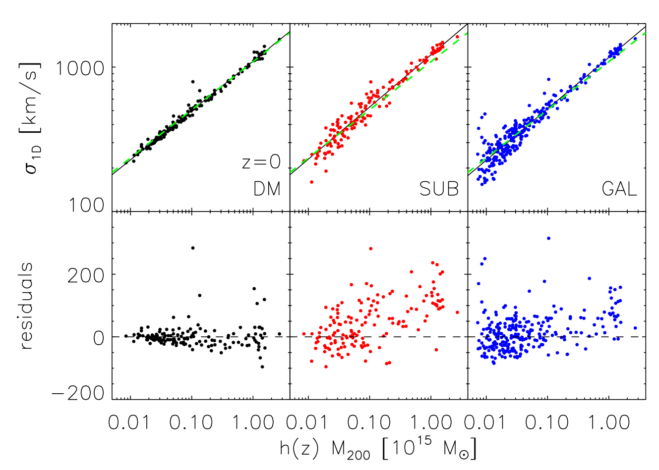
Figure 1: Top panels: velocity dispersion $\sigma_{\rm{1D}}$ (km s^-1) as a function of halo mass $\rm{h(z)}\,\rm{M}_{200}$ ($10^{15}\,\rm{M}_{\odot}$), for DM particles (left panels), subhalos (central panels), and galaxies (right panels), at z=0, in the AGN simulation sets. The dashed green line represents the theoretically expected relation $\sigma_{\rm{1D}}=1090\cdot(\rm{h(z)}\,\rm{M}_{200})^{1/3}$; the solid line in each panel represents the best-fit relation. Bottom panels: y-axis residuals of the DM particles (left), subhalos (centre), and galaxies (right), from the DM best-fit relation.

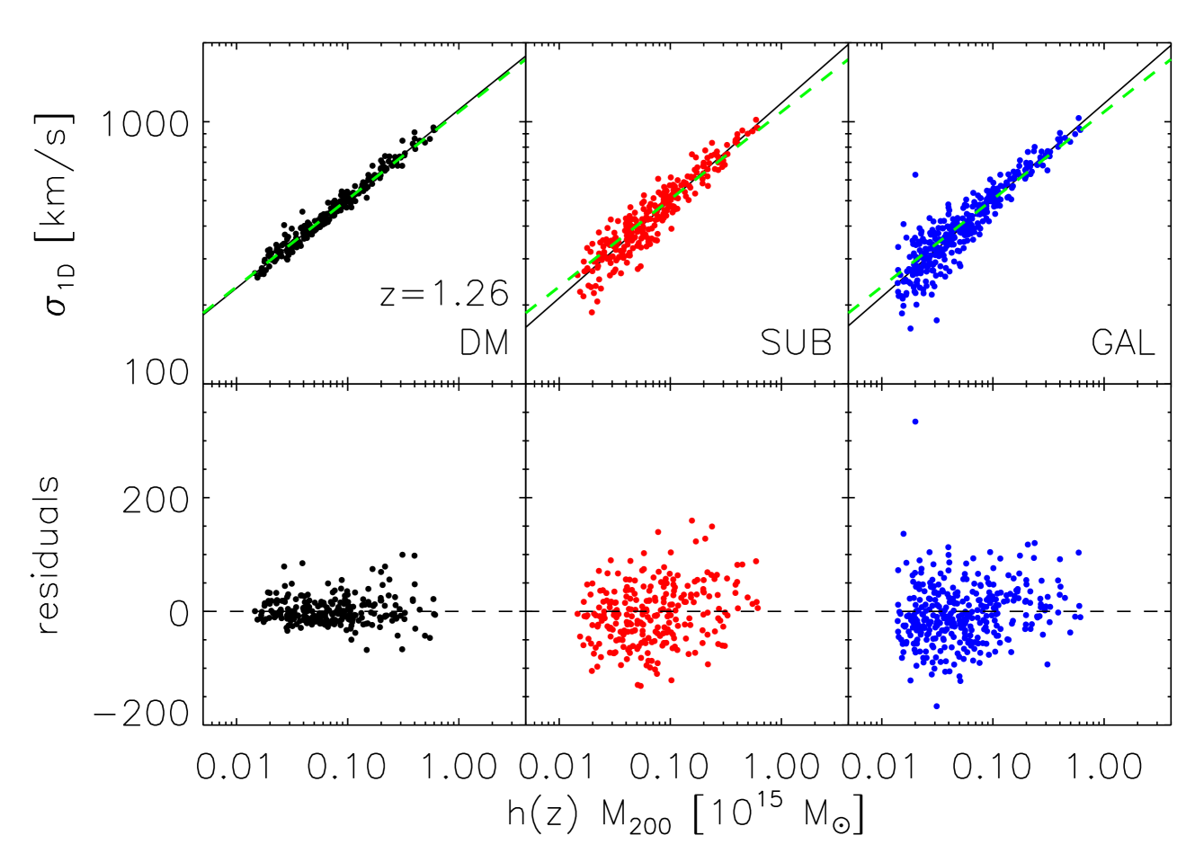
Figure 2: Same as Fig. 1 but for z=1.26.

In Fig. 3 we show the best fitting values of $A_{\rm{1D}}$ and $\alpha$ as a function of redshift, for different tracers in the AGN simulation, as an example. The slope $\alpha$ is confirmed to be consistent with the theoretically expected value $\alpha=1/3$. On the other hand, its value is significantly larger when using subhalos or galaxies as tracers. In any case the values of $\alpha$ and $A_{1D}$ do not generally show a significant dependence on z. Only in two cases (subhalos in the DM simulation and galaxies in the AGN simulation - see Appendix A) we do find (marginally) significant correlations between $\alpha$ and z, mostly driven by the point at z = 2. Even in these cases, $\alpha$ changes very little with redshift, $\simeq 4$% for the galaxies in the AGN simulation from z = 1.5 to z = 0. In fact, a model where $\alpha$ is constant with z provides an acceptable fit (in a $\chi^{2}$ sense) to all cases (also those not shown in Fig. 3). Since the variation of $A_{\rm{1D}}$ and $\alpha$ with z is not significant, we take the weighted averages of their values over all redshifts to characterise the $\sigma_{\rm{1D}}-\rm{M}_{200}$ relations of the different types of simulations and tracers (see Table 1 and Fig. 4).

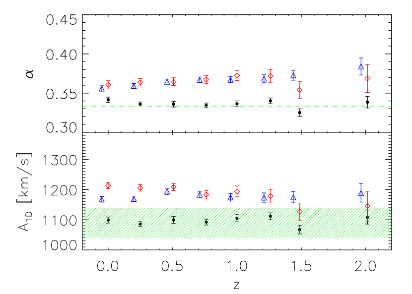
Figure 3: Average values of $\alpha$ and $A_{\rm{1D}}$ (see eq. 1) for halos in AGN simulations as a function of redshift, for different tracers, DM particle (black dots), subhalos (red diamonds), and galaxies (blue triangles). The dashed green line in the top panel is the theoretically expected value $\alpha=1/3$, the horizontal shaded area in the bottom panel indicates the expected theoretical range $A_{\rm{1D}}=1040$–1140 (see text). The data of galaxies have been shifted by $-0.05$ in z for the sake of clarity.

	$A_{1D}$ (km s-1)	$\alpha$
DM	$1094\pm 3.7$	$0.334\pm 0.0014$
NR	$1102\pm 3.4$	$0.336\pm 0.0021$
CSF	$1081\pm 4.1$	$0.329\pm 0.0021$
AGN	$1095\pm 4.4$	$0.336\pm 0.0015$
DM sub	$1244\pm 4.7$	$0.361\pm 0.0027$
NR sub	$1259\pm 5.3$	$0.364\pm 0.0030$
CSF sub	$1166\pm 5.1$	$0.362\pm 0.0018$
AGN sub	$1199\pm 5.2$	$0.365\pm 0.0017$
CSF gal	$1165\pm 6.7$	$0.355\pm 0.0025$
AGN gal	$1177\pm 4.2$	$0.364\pm 0.0021$

Table 1: Weighted average values over all redshifts of the parameters $A_{1D}$ and $\alpha$ defining the $\sigma_{1D}-M_{200}$ relation (see eq. (1)) for different simulation sets, for DM particles (top table), subhalos (middle table), and galaxies (bottom table).

In Fig. 4 we show the dependence of the parameters $\alpha$ and $A_{1D}$ on the physical processes included in the simulations. When considering DM particles as tracers, the $A_{\rm{1D}}$ values are well within the theoretically expected range, and the $\alpha$ values are close to the virial expectation 1/3, regardless of the baryonic physics implemented in the simulations. When considering subhalos or galaxies as tracers, the $\sigma_{\rm{1D}}$-$\rm{M}_{200}$ relations are significantly steeper ($\alpha>1/3$) than for DM particles and than expected theoretically. Furthermore, while the slope is nearly the same for all the simulation sets, with $\alpha\simeq 0.36$, the same does not hold for the normalization $A_{1D}$, this value being smaller when cooling and star formation are included. In each simulation set, the $\alpha$ and $A_{\rm{1D}}$ values are highest for the subhalos, and lowest for the DM particles, with the values for the galaxies being closer to those of the subhalos.

Both the $A_{1D}$ and the $\alpha$ values we find for the DM particles are in the range of the values listed by Evrard et al. (2008) and coming from the analysis of different simulations (see Table 4 in Evrard et al., 2008), most of which are DM-only. The comparison with Lau et al. (2010) is less straightforward, since they did find a z-dependence of the $\alpha$ parameter for DM particles. Taking an error-weighted average of the values they found at different redshifts, we obtain $A_{1D}=1103\pm 2$ km s^-1, $\alpha=0.325\pm 0.011$ for their non-radiative simulations, and $A_{1D}=1160\pm 9$ km s^-1, $\alpha=0.296\pm 0.012$ for their radiative simulation. Lau et al. (2010)’s $\sigma_{\rm{1D}}$–$\rm{M}_{200}$ relations are therefore flatter than ours, particularly so for the radiative simulations. We discuss these differences in Sect. 4.

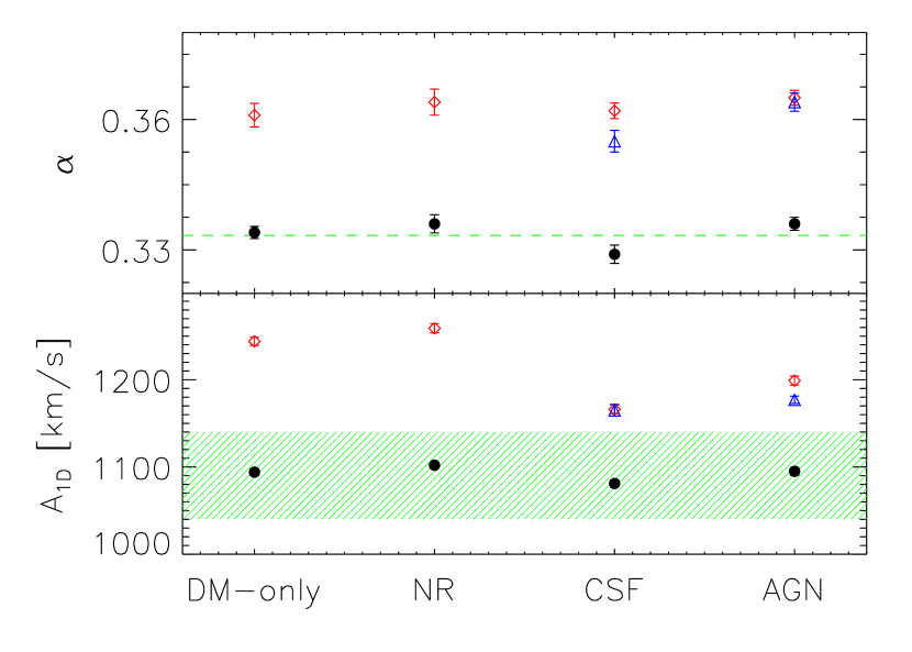
Figure 4: Values of $\alpha$ and $A_{\rm{1D}}$ (see eq. 1) averaged over all redshifts for different tracers - DM particle (black dots), subhalos (red diamonds), and galaxies (blue triangles) - for the different types of simulations. The dashed green line in the top panel is the theoretically expected value $\alpha=1/3$, the horizontal shaded area in the bottom panel indicates the expected theoretical range $A_{\rm{1D}}=1040$–1140 (see the text).

3.1 Scatter

An analysis of the scatter of the scaling relations is quite important for cosmological applications. It has been pointed out (see, e.g. Mortonson et al., 2011) that the so called Eddington bias causes the mass function to shift toward higher values of mass if the scatter in the scaling relation between mass and mass proxy is not properly taken into account. Furthermore we want to understand the nature of such scatter, that is whether it is intrinsic or mainly due to statistical uncertainties.

The best fit relation eq. (1) has been subtracted from the values of the velocity dispersion of the clusters for each simulation at each redshift. The result for the AGN set at z=0 is shown in Fig. 5 for the three tracers. The errors are associated to the biweight average value (Beers et al., 1990). In this figure the distribution of the residuals is also shown, along with the best fit gaussian curves and the reduced $\chi^{2}$ values of the fits. The residuals appear to be normally distributed, substructures and galaxies having a wider distribution.

The scatter appears to be independent of cluster mass, as well as of redshift and the type of simulation as shown in top panels of Fig. 6, the only difference being in the tracer used to build the $\sigma_{\rm{1D}}$–$\rm{M}_{200}$ relation. When using DM particles the scatter is around $5\%$, while using substructures or galaxies it is around $12\%$.

In order to understand the nature of the scatter, that is whether it is intrinsic or statistical, we have tried to compute the intrinsic scatter following Williams et al. (2010). Performing a linear fit of the $\log\sigma_{1D}-\log\rm{M}_{200}$ relation, the intrinsic scatter is considered as a parameter that minimizes $\chi^{2}=\sum_{i=1}^{N_{clus}}[y_{i}-(a\cdot x_{i}+b)]^{2}/[\epsilon_{y,i}^{2}+a^{2}\cdot\epsilon_{x,i}^{2}+\sigma_{int}^{2}]$, where $y=a\cdot x+b$ is the linear relation, $\epsilon_{x,i}$ and $\epsilon_{y,i}$ are the uncertainties on the x and y quantities and $\sigma_{int}$ is the intrinsic scatter. In order to estimate the value of the intrinsic scatter and its uncertainty, we performed 1000 bootstrap resamplings of the couples of values $(\rm{M}_{200},\sigma_{1D})$, each time computing the intrinsic scatter estimate. In a first time, we have evaluated the intrinsic scatter in 4 bins of mass, but we found no mass dependence. Therefore we have evaluated it using all the data. The values of velocity dispersion evaluated using DM particles have been obtained using a huge number of objects, hence the statistical uncertainty is very small. The $5\%$ scatter is therefore entirely intrinsic. On the other hand velocity dispersions estimates using substructures and galaxies are based on relatively small numbers of objects, and statistical uncertainties dominate the scatter. The resulting intrinsic scatter for these tracers turns out to be quite small and consistent with the value found for DM particles.

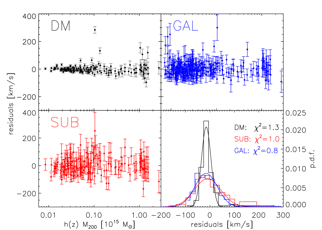
Figure 5: Residuals of the velocity dispersion after subtracting the best fit relation eq. (1) for the AGN set at z=0, for the three tracers as indicated in the panels. The distributions of residuals for the three tracers is also shown in the bottom right panel, along with the best fit gaussian curves and the reduced $\chi^{2}$ of the fits.

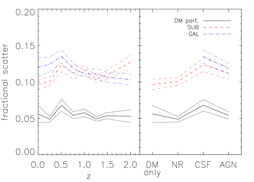
Figure 6: Left panel: Fractional scatter as a function of redshift in the AGN set. Black solid line refers to the value computed by using DM particles, red dashed and blue dash-dotted by using substructures and galaxies, respectively. The thinner lines are the confidence intervals. Right panel: Fractional scatter as a function of the type of simulation at z=0. Lines and colours are the same as in the left panel.

3.2 Velocity bias

The difference between the $\sigma_{\rm{1D}}$–$\rm{M}_{200}$ relations established for DM particles, on one side, and subhalos and galaxies, on the other side implies that subhalos and galaxies have a higher velocity dispersion than DM particles in high mass halos. Since the relation is steeper for subhalos and galaxies than for DM particles, the opposite may occur in halos of low masses. To examine how $\sigma_{\rm{1D}}$ changes in halos of different masses when using different implementations of baryonic physics, here we analyse the velocity bias, i.e. the ratio between the velocity dispersions of subhalos (galaxies) and DM particles, $\rm{b_{v}}=\sigma_{\rm{sub}}/\sigma_{\rm{DM}}$ ($\rm{b_{v}}=\sigma_{\rm{gal}}/\sigma_{\rm{DM}}$, respectively), for two subsamples of halos, one with masses $\rm{h(z)}\rm{M}_{200}<10^{14}\rm{M}_{\odot}$, and the other with masses $\rm{h(z)}\rm{M}_{200}>3\cdot 10^{14}\rm{M}_{\odot}$ (the low- and high-mass samples hereafter). The average $\rm{b_{v}}$ values as a function of redshift are shown in Fig. 7 and 8, for subhalos and galaxies in different simulation sets, separately for the halos in the low-mass sample (left panels) and for the halos in the high-mass sample (right panels).

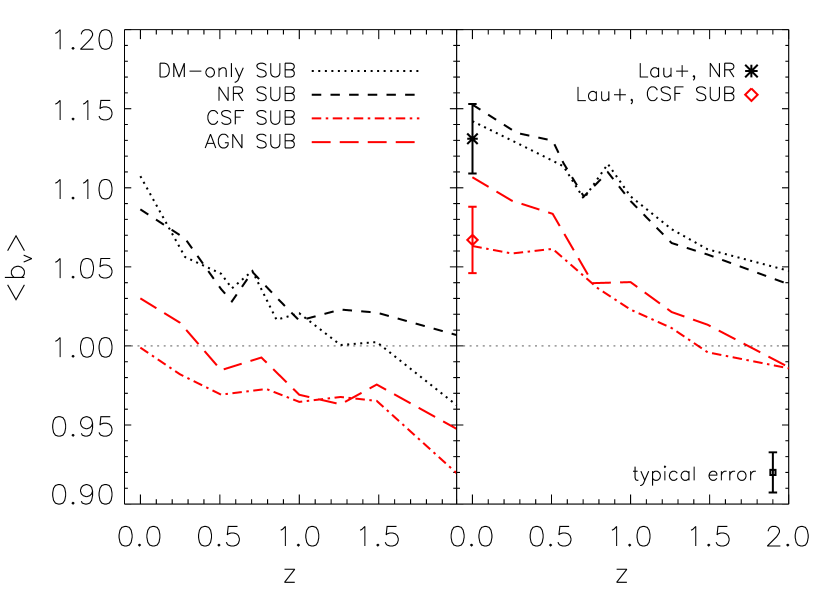
Figure 7: Average values of the velocity bias for subhalos, as a function of redshift, for halos in the low-mass sample (left panel) and in the high-mass sample (right panel). Dotted line refers to substructures in the DM set, short black dashed line refers to substructures in the NR set, the other lines refer to substructures of the CSF and AGN sets, as indicated in the legend. Error-bars on the bias values are not shown for the sake of clarity. A typical error-bar is shown at the bottom-right of the right panel. The other points with error bars are the z = 0 values from Lau et al. (2010). The legend in the right panel identifies the different symbols as representative of the non-radiative simulations (NR), and the CSF simulations of Lau et al. (2010).

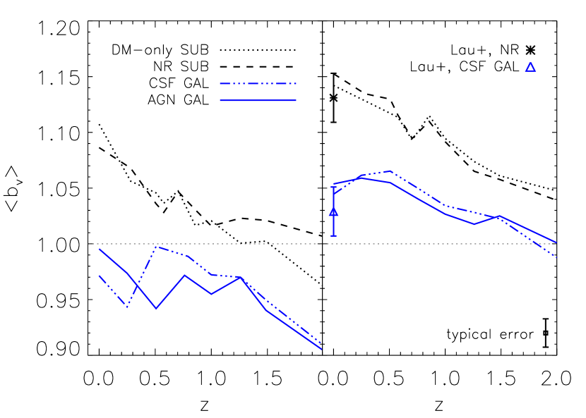
Figure 8: Same as Fig. 7 but for galaxies rather than substructures.

The bias is on average higher for the high-mass sample halos, and at lower redshifts. A remarkable change in the bias appears when introducing cooling and star formation. In fact the biases are higher for substructures in the DM and in non-radiative simulations (NR) than in the radiative ones (CSF, AGN), both when using substructures and galaxies, reflecting again the importance of the cooling and the feedback processes in the dynamics.

In Fig. 7 and 8 we also show the values found by Lau et al. (2010). At z = 0, the sample of Lau et al. (2010) and ours have similar mass distributions and there is a good agreement (within the error bars) between their $\rm{b_{v}}$ values and ours, separately for the different types of simulations and for the different tracers. The comparison between our data and those in Lau et al. (2010) at $\rm{z}>0$ is not shown because it is not straightforward: Lau et al. (2010) follow the same halos at different redshifts by always considering the most massive progenitors of the halos selected at z = 0, whereas we consider all halos above a given mass cut at any given redshift. Taken at face value, the biases they find at higher z are smaller than those we find, and this difference might be related to a strong overcooling present in their simulations, making their subhalos very resistant to tidal disruption.

3.3 Dynamical processes in halos

The above results show how the relative kinetic energy content in subhalos (or galaxies) and the diffuse DM component varies with redshift, halo mass, and the type of simulations. Here we provide an interpretation of these results in terms of the dynamical processes that are effective in clusters and groups, i.e. dynamical friction, merging with the central galaxy, tidal disruption, and accretion from the surrounding large-scale structure, and how these processes depend on the physics implemented in the simulations.

A better understanding of the physical cause of the differences in the $\sigma_{\rm{1D}}$-$\rm{M}_{200}$ relation and of the velocity biases analysed in the two previous sections can be obtained by examining the probability distribution function for the modulus of the velocity of the different tracers. These distributions are shown in Fig. 9 for the CSF and AGN simulations, at z = 0 and 1.26, separately for the low- and high-mass samples.

The velocity distribution of DM particles (solid black lines in Fig. 9) appears to be single-peaked, but only for the low-mass sample. The DM particle velocity distribution for the high-mass sample is flat-topped and sometimes double-peaked. These features, present in all the different types of simulations, appear to be more pronounced for the velocity distributions of subhalos (dashed red lines) and galaxies (dotted blue lines), and depend on the physics implemented in the simulations. The difference in the velocity distributions of DM particles, subhalos, and galaxies is at the origin of the velocity biases and the differences in their $\sigma_{\rm{1D}}$-$\rm{M}_{200}$ relations. Hereafter we interpret the effect of the dynamical processes that shape these velocity distributions.

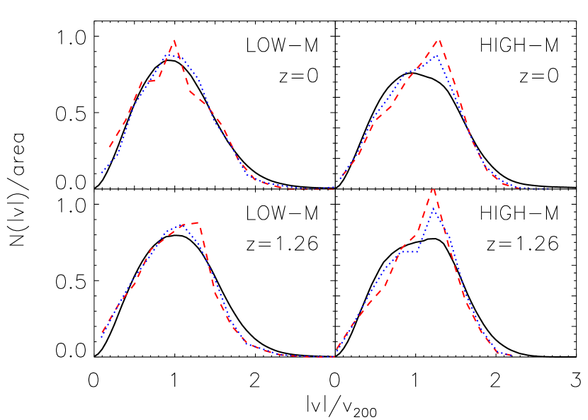
Figure 9: Top panels: The velocity distributions for the CSF simulations for the low-mass sample (left panels) and the high-mass sample (right panels) at $z=0$ (top panels) and $z=1.26$ (bottom panels) for DM particles (solid black lines), subhalos (dashed red lines) and galaxies (dotted blue lines). All distributions are normalised to their integrals. Bottom panels: same as top panels but for the AGN simulations.

A flat-topped or double-peaked velocity distribution is the signature of ongoing mergers and infall of matter into the halos, which tends to populate the high-velocity part of the velocity distributions (see, e.g. Diemand et al., 2004; Wang et al., 2005; Wetzel, 2011; Ribeiro et al., 2011). With time, the velocity distribution relaxes via phase-mixing and dynamical relaxation and approaches a single Maxwellian (e.g. Faltenbacher & Diemand, 2006; Lapi & Cavaliere, 2011, and references therein).

The relative importance of the relaxed and unrelaxed velocity distributions depends on how strong the matter infall rate is. Higher-mass halos are dynamically younger, and undergo significant matter infall until more recent times than lower-mass halos (e.g. Lapi & Cavaliere, 2009; Faltenbacher & White, 2010). Hence in higher-mass halos the unrelaxed, high-velocity component is more important than in lower-mass clusters, as we see in Fig. 9.

The velocity distributions of subhalo and galaxies is different from those of DM particles, because of additional dynamical processes that leave the DM particle distributions unaffected. One is the dynamical friction, leading to a decrease in the orbital energy, hence to an approach to the cluster centre and a decrease in velocity, eventually followed by merger with the central cluster galaxy (e.g. Boylan-Kolchin et al., 2008; Wetzel & White, 2010). The other process is tidal disruption, caused by the integral of tidal interactions leading to mass losses (e.g. Diemand et al., 2004). These two processes are related. On one hand, dynamical friction becomes ineffective when tidal mass losses become important (e.g. Faltenbacher & Mathews, 2007), because dynamical friction is more effective for more massive objects. On the other hand, tidal mass losses are enhanced by dynamical friction, since they are more effective in slow-moving subhalos (and galaxies) than their fast-moving counterparts (Diemand et al., 2004). Hence dynamical friction is likely to be more effective at the first orbit of a subhalo (or galaxy) (Faltenbacher & Mathews, 2007), while tidal disruption may take several orbits.

Dynamical friction tends to increase the low-velocity tail of the distribution. A possible signature of this effect is visible in the velocity distributions of subhalos and galaxies at high-z in Fig. 9. On the other hand, the removal of the slowest subhalos (or galaxies) by tidal disruption or merger with the central galaxy tends to decrease the low-velocity tail of the distribution. This is likely to occur in the relaxed component of the global velocity distribution, since subhalos (and galaxies) in the relaxed component have spent more time orbiting their parent halos than the recently infallen, unrelaxed population. The resulting velocity distribution will then appear to be double peaked, one low-velocity peak being due to the relaxed component, depopulated by tidal stripping, and another high-velocity peak due to the infalling population, that has not yet experienced significant tidal mass losses. This is particularly evident in higher-mass halos, in which the infall rate is higher (at given z) than in lower-mass halos. The resulting asymmetric velocity distribution is visible in Fig. 9 (dashed red and dotted blue lines).

These processes are dependent on the physical processes and feedback implemented in the simulations. In fact in Fig. 9 one can note that the velocity distributions of galaxies and subhalos in the CSF simulation sets are both closer to the velocity distributions of DM particles, than the corresponding ones in the AGN simulation sets. This occurs because baryon cooling tends to make galaxies and subhalos more resistant against tidal disruption (e.g. Weinberg et al., 2008; Lau et al., 2010). However cooling efficiency is reduced in simulations including AGN feedback thus making halos less compact and galaxies more fragile than in the over-cooled CSF simulations.

Yet another difference is visible in Fig. 9, namely the velocity distribution for galaxies in the AGN sets is slightly closer to the distribution of DM particles than that of subhalos. This is due to the different mass limit we use to select galaxies and subhalos (see Sect. 2). In our samples, subhalos selected by means of total bound mass are on average objects of higher mass than subhalos selected by means of stellar mass, hence they are subject to stronger dynamical friction, slowing them down and making them more easily subject to tidal disruption. Our result is reminiscent of that of Faltenbacher & Diemand (2006) who found that the velocity distribution of galaxies is quite similar to that of DM particles when selecting objects by their mass at accretion, i.e. before tidal stripping operates, as pointed out also by Lau et al. (2010).

The processes so far discussed provide a frame for a better understanding of Fig. 7 and 8. At fixed galaxy mass, dynamical friction is more efficient in low-mass clusters and at high redshifts, before tidal stripping decreases galaxy masses. Therefore dynamical friction tends to create a velocity bias $<1$ in low mass, high-z systems, while leaving almost unaffected high mass clusters. Tidal stripping is more efficient on slow moving galaxies, which are stripped and eventually disrupted (or removed from a mass-limited sample), and operates at all times. This causes an increase of the bias with time. This has the effect of erasing the initial dynamical-friction bias in low-mass clusters and creating a bias $>1$ in high-mass clusters as we approach $\rm{z}=0$.

An important rôle in these processes may also be played by galaxy orbits. In Fig. 10 we show the velocity anisotropy profiles for the different tracers, in low- and high-mass systems, for z=0 and 1.26. For lack of sufficient number of substructures and galaxies in each system, the profiles for these tracers are computed for stacks of all systems, where substructure and galaxy velocities have been scaled by each system $\rm{v}_{200}$ before stacking. With this procedure, richer clusters weigh more in the final profile. For the DM particles we are not limited by poor statistics, so we derive the anisotropy profiles individually for each halo, and then take an average. For consistency with what was done for the substructures and galaxies, the average is weighted by the number of substructures present in each cluster. Fig. 10 shows that orbits are more radially anisotropic in high-mass than in low-mass systems (as already shown by Wetzel, 2011). Understanding the reason for this difference (and for the redshift evolution clearly visible in the same figure) is beyond the scope of this paper, although we suspect that it might be related to the younger dynamical age of higher mass clusters (as suggested by, e.g., Biviano & Poggianti, 2009, and references therein). What is relevant in this context is that galaxies on more radial orbits reach closer to the cluster centre and therefore suffer from stronger tidal stripping effects. The different orbital anisotropy of galaxies contribute to create a higher velocity bias in high-mass relative to low-mass clusters.

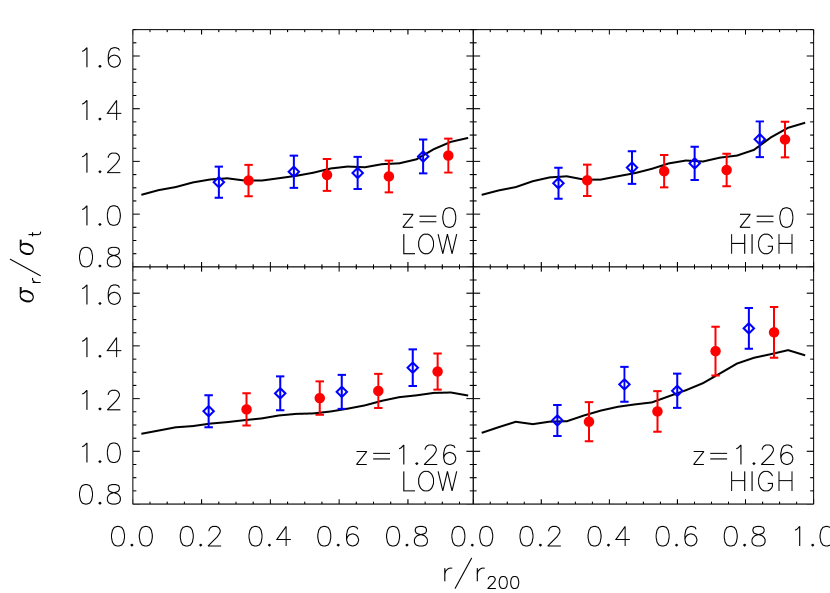
Figure 10: Velocity anisotropy as a function of the cluster center, for the AGN set. Top panels refer to z=0, bottom panels to z=1.26. Panels on the left are relative to the low-mass sample, panels on the right to the high-mass sample. Red points refer to the results obtained using subhalos, while blue diamonds using galaxies. The four bins are built in such a way that within each bin there is the same number of objects. Galaxies diamonds have been shifted by -0.05 in redshift for the sake of clarity. The black solid line refers to the results obtained using DM particles.

4 Discussion and conclusions

We determined the $\sigma_{\rm{1D}}$-$\rm{M}_{200}$ relation for DM particles, subhalos, and galaxies in cluster- and group-sized halos extracted from $\Lambda$CDM cosmological simulations. We analysed four sets of simulations carried out for the same halos: one DM-only, one with non-radiative gas, and another two with gas cooling, star formation and galactic ejecta triggered by SN winds, one of the two also including the effect of AGN feedback.

The main results of our analysis can be summarised as follows.

• We confirm that the $\sigma_{1D}-M_{200}$ relations for the DM particles are consistent with the theoretical expectation from the virial relation, assuming NFW halo mass profiles, with reasonable values of concentration and velocity anisotropy.

• The intercepts at $10^{15}\rm{M}_{\odot}$ and slopes of the logarithmic $\sigma_{\rm{1D}}$-$\rm{M}_{200}$ relations derived using subhalos and galaxies as tracers of the potential are always higher than those derived using DM particles. We do not find a significant dependence of the $\sigma_{\rm{1D}}$-$\rm{M}_{200}$ relations on redshift, but we do find a dependence on the kind of simulation, the radiative ones having a higher value of the normalization.

• The $\sigma_{\rm{1D}}$-$\rm{M}_{200}$ relations for the DM particles are consistent with those found by Evrard et al. (2008). On the other hand the relations we find for all the tracers are steeper than those derived by Lau et al. (2010). This difference might be caused by the narrower halo mass range explored by Lau et al. (2010).

• The differences in the $\sigma_{\rm{1D}}$-$\rm{M}_{200}$ relations for the different tracers of the halo gravitational potential and for the different physics implemented are due to dynamical processes taking place in the halos. In fact dynamical friction and tidal disruption act on substructures and galaxies but not on DM particles. Dynamical friction slows down a substructure or a galaxy before it suffers mass loss due to tidal stripping. Dynamical friction is therefore more efficient at high-z. It is also more efficient in lower-mass clusters for given galaxy mass. Tidal stripping, on the other hand, is more efficient in higher-mass clusters, where galaxies move on more radial orbits (hence with smaller pericenter radii). As a result, velocity biases are created in the substructure and galaxy populations, relative to the DM particles, and these biases are $\leq 1$ for low-mass systems and $\geq 1$ for high-mass systems, and increasing with time, leading to the observed differences in the $\sigma_{\rm{1D}}$-$\rm{M}_{200}$ relations of different tracers.

• In order to correctly reproduce such processes, a detailed implementation of the baryonic physics must be used in the simulations. In fact the presence of baryonic matter makes halos more resistant against tidal disruption (e.g. Weinberg et al., 2008). In this way in simulations with cooling and star formation there is a higher fraction of survivors among the slow moving subhalos, reflecting in a lower value of the normalization on the $\sigma_{\rm{1D}}$-$\rm{M}_{200}$ relation.

• We analysed the scatter in the $\sigma_{1D}-\rm{M}_{200}$ relation, finding a value of around $5\%$ for DM particles and $12\%$ for substructures and galaxies. The intrinsic scatter, after accountinbg for the statistical errors in the $\sigma_{1D}$ measurements, appears to be $\lesssim 5\%$, independently of the tracer.

Such a small scatter in the $\sigma_{1D}-\rm{M}_{200}$ relation potentially makes $\sigma_{1D}$ a very good proxy for the mass, via inversion of eq. (1): $M_{200}/10^{15}\rm{M}_{\odot}=(\sigma_{1D}/A_{1D})^{(1/\alpha)}/h(z)$. However, $A_{1D}$ and $\alpha$ are significantly different for the different tracers (DM particles, substructures, galaxies). Using the values obtained for one tracer to infer cluster masses from the $\sigma_{1D}$ of a different tracer can lead to systematic errors of up to $\sim 30\%$. In comparison, the effect of using different baryonic physics for the same tracer has a much smaller effect on the mass estimates obtained from $\sigma_{1D}$ ($\lesssim 7\%$, see Table 2). The presence of scatter, even though small, makes possible the applicability of the scaling relation only in a statistical sense, not for mass estimates of single objects.

simulation	tracer	$\sigma_{1D}=300$ km/s	$\sigma_{1D}=900$ km/s
DM	DM part	0.029	0.774
NR	DM part	0.029	0.760
CSF	DM part	0.028	0.796
AGN	DM part	0.029	0.775
DM	sub	0.027	0.567
NR	sub	0.027	0.552
CSF	sub	0.033	0.679
AGN	sub	0.031	0.633
CSF	gal	0.030	0.671
AGN	gal	0.032	0.665

Table 2: Masses (in $10^{15}\rm{M}_{\odot}$) of clusters at z=0 predicted from the $\sigma_{1D}-\rm{M}_{200}$ relation for two values of $\sigma_{1D}$, 300 $m/s$ and 900 $m/s$.

The results of this paper show that good knowledge of the $\sigma_{1D}-\rm{M}_{200}$ relation in 6D phase space is fundamental before one could apply this relation to observational samples. Projection effects and the presence of interlopers can significantly affect the accuracy and reliability of the mass estimate (e.g. Cen, 1997; Biviano et al., 2006). We plan to consider these effects in detail, in a forthcoming work, using simulations with a proper implementation of baryonic physics and galaxies as tracers.

Appendix A Plots for other models

In this appendix we report the plots showing the redshift dependence of the slope and the intercept of eq. (1) as well as the velocity distributions of the tracers for all simulation sets not already shown before in the main text.

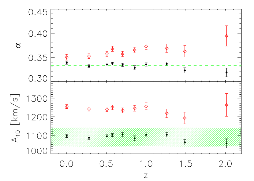
Figure 11: Same as Fig. 3 for the DM set.

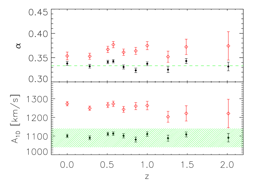
Figure 12: Same as Fig. 3 for the NR set.

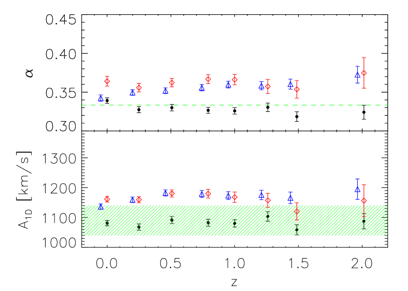
Figure 13: Same as Fig. 3 for the CSF set.

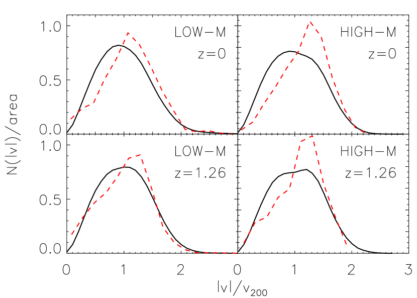
Figure 14: Same as Fig. 9 for the DM set.

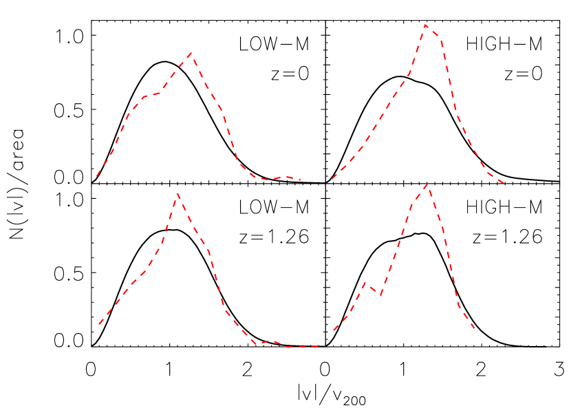
Figure 15: Same as Fig. 9 for the NR set.

References

- Allen et al. (2011) Allen S. W., Evrard A. E., Mantz A. B., 2011, ARAA, 49, 409
- Arnaud et al. (2010) Arnaud M., Pratt G. W., Piffaretti R., Böhringer H., Croston J. H., Pointecouteau E., 2010, A&A, 517, A92
- Beers et al. (1990) Beers T., Flynn K., Gebhardt K., 1990, aj, 100, 32
- Biviano et al. (2006) Biviano A., Murante G., Borgani S., Diaferio A., Dolag K., Girardi M., 2006, A&A, 456, 23
- Biviano & Poggianti (2009) Biviano A., Poggianti B. M., 2009, A&A, 501, 419
- Bonafede et al. (2011) Bonafede A., Dolag K., Stasyszyn F., Murante G., Borgani S., 2011, MNRAS, 418, 2234
- Borgani & Kravtsov (2011) Borgani S., Kravtsov A., 2011, Adv. Sci. Letters, 4, 204
- Boylan-Kolchin et al. (2008) Boylan-Kolchin M., Ma C., Quataert E., 2008, MNRAS, 383, 93
- Cen (1997) Cen R., 1997, ApJ, 485, 39
- Chabrier (2003) Chabrier G., 2003, PASP, 115, 763
- Chandrasekhar (1943) Chandrasekhar S., 1943, ApJ, 97, 255
- Diemand et al. (2004) Diemand J., Moore B., Stadel J., 2004, MNRAS, 352, 535
- Dolag et al. (2009) Dolag K., Borgani S., Murante G., Springel V., 2009, MNRAS, 399, 497
- Duffy et al. (2008) Duffy A. R., Schaye J., Kay S. T., Dalla Vecchia C., 2008, MNRAS, 390, L64
- Esquivel & Fuchs (2007) Esquivel O., Fuchs B., 2007, MNRAS, 378, 1191
- Ettori et al. (2002) Ettori S., De Grandi S., Molendi S., 2002, A&A, 391, 841
- Evrard et al. (2008) Evrard A. E., et al., 2008, ApJ, 672, 122
- Fabjan et al. (2010) Fabjan D., Borgani S., Tornatore L., Saro A., Murante G., Dolag K., 2010, MNRAS, 401, 1670
- Faltenbacher & Diemand (2006) Faltenbacher A., Diemand J., 2006, MNRAS, 369, 1698
- Faltenbacher et al. (2005) Faltenbacher A., Kravtsov A. V., Nagai D., Gottlöber S., 2005, MNRAS, 358, 139
- Faltenbacher & Mathews (2007) Faltenbacher A., Mathews W. G., 2007, MNRAS, 375, 313
- Faltenbacher & White (2010) Faltenbacher A., White S. D. M., 2010, ApJ, 708, 469
- Ferland et al. (1998) Ferland G. J., Korista K. T., Verner D. A., Ferguson J. W., Kingdon J. B., Verner E. M., 1998, PASP, 110, 761
- Gao et al. (2008) Gao L., Navarro J. F., Cole S., Frenk C. S., White S. D. M., Springel V., Jenkins A., Neto A. F., 2008, MNRAS, 387, 536
- Gill et al. (2004) Gill S. P. D., et al., 2004, MNRAS, 351, 410
- Haardt & Madau (2001) Haardt F., Madau P., 2001, in D. M. Neumann & J. T. V. Tran ed., Clusters of Galaxies and the High Redshift Universe Observed in X-rays Modelling the UV/X-ray cosmic background with CUBA
- Hoekstra (2003) Hoekstra H., 2003, MNRAS, 339, 1155
- Katgert et al. (2004) Katgert P., Biviano A., Mazure A., 2004, ApJ
- Kay et al. (2012) Kay S. T., Peel M. W., Short C. J., Thomas P. A., Young O. E., Battye R. A., Liddle A. R., Pearce F. R., 2012, MNRAS, 422, 1999
- Kravtsov & Borgani (2012) Kravtsov A. V., Borgani S., 2012, ARAA, 50, 353
- Kravtsov et al. (2006) Kravtsov A. V., Vikhlinin A., Nagai D., 2006, ApJ, 650, 128
- Lapi & Cavaliere (2009) Lapi A., Cavaliere A., 2009, ApJ, 692, 174
- Lapi & Cavaliere (2011) Lapi A., Cavaliere A., 2011, ApJ, 743, 127
- Lau et al. (2010) Lau E. T., Nagai D., Kravtsov A. V., 2010, ApJ, 708, 1419
- Laureijs et al. (2011) Laureijs R., Amiaux J., Arduini S., Auguères J. ., Brinchmann J., Cole R., Cropper M., Dabin C., Duvet L., Ealet A., et al. 2011, Euclid Definition Study Report
- Limousin et al. (2007) Limousin M., Kneib J. P., Bardeau S., Natarajan P., Czoske O., Smail I., Ebeling H., Smith G. P., 2007, A&A, 461, 881
- Łokas & Mamon (2001) Łokas E. L., Mamon G. A., 2001, MNRAS, 321, 155
- Mamon et al. (2010) Mamon G. A., Biviano A., Murante G., 2010, A&A, 520, A30
- Mauduit & Mamon (2007) Mauduit J.-C., Mamon G. A., 2007, A&A, 475, 169
- Mauduit & Mamon (2009) Mauduit J.-C., Mamon G. A., 2009, A&A, 499, 45
- Mortonson et al. (2011) Mortonson M. J., Hu W., Huterer D., 2011, Phys. Rev. D, 83, 023015
- Natarajan et al. (2002) Natarajan P., Kneib J.-P., Smail I., 2002, ApJ, 580, L11
- Padovani & Matteucci (1993) Padovani P., Matteucci F., 1993, ApJ, 416, 26
- Popesso et al. (2007) Popesso P., Biviano A., Böhringer H., Romaniello M., 2007, A&A, 464, 451
- Ribeiro et al. (2011) Ribeiro A. L. B., Lopes P. A. A., Trevisan M., 2011, MNRAS, 413, L81
- Rozo et al. (2009) Rozo E., Rykoff E. S., Evrard A., Becker M., McKay T., Wechsler R. H., Koester B. P., Hao J., Hansen S., Sheldon E., Johnston D., Annis J., Frieman J., 2009, ApJ, 699, 768
- Saro et al. (2012) Saro A., Bazin G., Mohr J., Dolag K., 2012, ArXiv e-prints
- Sijacki et al. (2007) Sijacki D., Springel V., Di Matteo T., Hernquist L., 2007, MNRAS, 380, 877
- Springel (2005) Springel V., 2005, MNRAS, 364, 1105
- Springel et al. (2005) Springel V., Di Matteo T., Hernquist L., 2005, MNRAS, 361, 776
- Springel & Hernquist (2003) Springel V., Hernquist L., 2003, MNRAS, 339, 289
- Springel et al. (2001) Springel V., Yoshida N., White S. D. M., 2001, New Astronomy, 6, 79
- Stanek et al. (2010) Stanek R., Rasia E., Evrard A. E., Pearce F., Gazzola L., 2010, ApJ, 715, 1508
- Tormen et al. (1997) Tormen G., Bouchet F. R., White S. D. M., 1997, MNRAS, 286, 865
- Tornatore et al. (2007) Tornatore L., Borgani S., Dolag K., Matteucci F., 2007, MNRAS, 382, 1050
- Wang et al. (2005) Wang H. Y., Jing Y. P., Mao S., Kang X., 2005, MNRAS, 364, 424
- Weinberg et al. (2008) Weinberg D. H., Colombi S., Davé R., Katz N., 2008, ApJ, 678, 6
- Wetzel (2011) Wetzel A. R., 2011, MNRAS, 412, 49
- Wetzel & White (2010) Wetzel A. R., White M., 2010, MNRAS, 403, 1072
- White et al. (2011) White M., et al., 2011, ApJ, 728, 126
- Wiersma et al. (2009) Wiersma R. P. C., Schaye J., Smith B. D., 2009, MNRAS, 393, 99
- Williams et al. (2010) Williams M. J., Bureau M., Cappellari M., 2010, MNRAS, 409, 1330
- Williamson et al. (2011) Williamson R., Benson B. A., High F. W., Vanderlinde K., Ade P. A. R., Aird K. A., Andersson K., Armstrong R., Ashby M. L. N., Bautz M., Bazin G., Bertin E., Bleem L. E., Bonamente M., 2011, ApJ, 738, 139
- Wojtak et al. (2008) Wojtak R., Łokas E. L., Mamon G. A., Gottlöber S., Klypin A., Hoffman Y., 2008, MNRAS, 388, 815