Observations of Feedback from Radio-Quiet Quasars:
I. Extents and Morphologies of Ionized Gas Nebulae

Abstract

Black hole feedback – the strong interaction between the energy output of supermassive black holes and their surrounding environments – is routinely invoked to explain the absence of overly luminous galaxies, the black hole vs. bulge correlations and the similarity of black hole accretion and star formation histories. Yet direct probes of this process in action are scarce and limited to small samples of active nuclei. In this paper we present Gemini Integral Field Unit observations of the distribution of ionized gas around luminous, obscured, radio-quiet quasars at $z\sim 0.5$. We detect extended ionized gas nebulae via [O iii]$\lambda$5007Å emission in every case, with a mean diameter of 28 kpc. These nebulae are nearly perfectly round, with H$\beta$ surface brightness declining $\propto R^{-3.5\pm 1.0}$. The regular morphologies of nebulae around radio-quiet quasars are in striking contrast with lumpy or elongated [O iii] nebulae seen around radio galaxies at low and high redshifts. We present the uniformly measured size-luminosity relationship of [O iii] nebulae around Seyfert 2 galaxies and type 2 quasars spanning six orders of magnitude in luminosity and confirm the flat slope of the correlation ($R_{\rm[O~{}{\scriptscriptstyle III}]}\propto L_{\rm[O~{}{\scriptscriptstyle III}]}^{0.25\pm 0.02}$). We propose a model of clumpy nebulae in which clouds that produce line emission transition from being ionization-bounded at small distances from the quasar to being matter-bounded in the outer parts of the nebula. The model – which has a declining pressure profile – qualitatively explains line ratio profiles and surface brightness profiles seen in our sample. It is striking that we see such smooth and round large-scale gas nebulosities in this sample, which are inconsistent with illuminated merger debris and which we suggest may be the signature of accretion energy from the nucleus reaching gas at large scales.

1 Introduction

Feedback from accreting black holes has become a key element in modeling galaxy evolution (Tabor & Binney, 1993; Silk & Rees, 1998; Springel et al., 2005). For one thing, regulatory mechanisms are needed to keep massive galaxies from forming too many stars and becoming overly massive or blue at late times (Thoul & Weinberg, 1995; Croton et al., 2006). Black holes are natural candidates because even a small fraction of the binding energy of the infalling material is in principle sufficient to liberate the galaxy-scale gas from the galaxy potential. The discovery that the masses of supermassive black holes in inactive galaxies strongly correlate with the velocity dispersions and masses of their hosts’ stellar bulges (Magorrian et al., 1998; Gebhardt et al., 2000; Ferrarese & Merritt, 2000; Tremaine et al., 2002; Marconi & Hunt, 2003; Häring & Rix, 2004; Gültekin et al., 2009; McConnell et al., 2011) also suggests that the energy output of the black hole in its most active – quasar – phase must be somehow coupled to the gas from which the stars form (Hopkins et al., 2006). The problem remains to find direct observational evidence of black hole-galaxy self-regulation and to obtain measurements of feedback energetics.

In some situations, accretion energy clearly has had an impact on the large-scale environment of the accreting black hole. For instance, radio jet activity in massive elliptical galaxies and brightest cluster galaxies deposits energy into the hot gas envelope of the cluster (McNamara & Nulsen, 2007; Randall et al., 2011). Likewise, there is clear evidence that powerful radio jets entrain warm gas and carry significant amounts of material out of their host galaxies (van Breugel et al., 1986; Tadhunter, 1991; Whittle, 1992; Villar-Martín et al., 1999; Nesvadba et al., 2006, 2008; Fu & Stockton, 2009), and the observed entropy profiles of galaxy clusters can be explained by invoking a heating mechanism from their central radio-loud quasars to reduce the gas supply from the hot intra-cluster medium (Scannapieco & Oh, 2004; Voit, 2005; Voit & Donahue, 2005; Donahue et al., 2006). Nevertheless, as radio-loud quasars only represent a small fraction ($\sim 10\%$) of the entire quasar population, invoking this mechanism as the primary mode of limiting galaxy mass would require all galaxies to have undergone a radio-loud phase – a conjecture which lacks direct evidence and contradicts a theoretical paradigm in which radio-loudness is determined by the spin of the black hole (Tchekhovskoy et al., 2010).

Nuclear activity is known to drive outflows on small scales (Crenshaw et al., 2003; Ganguly & Brotherton, 2008), perhaps via the radiation pressure of the quasar (Murray et al., 1995; Proga et al., 2000). Broad absorption-line troughs are seen in $\sim 10-20\%$ of luminous quasars (Reichard et al., 2003), or alternatively the outflows are ubiquitous, and this frequency simply reflects their covering factors (Weymann et al., 1981; Gallagher et al., 2007; Shen et al., 2008). The velocities in broad absorption lines can be up to $\sim 10,000$ km/s, suggesting that high energies are involved, but in practice velocity is the only physical parameter in such outflows which is directly measurable. Careful photo-ionization modeling of specific absorption features (Arav et al., 2008) demonstrated that in several objects the outflow appears to extend out to several kpc from the nucleus and to carry a large amount of kinetic energy and momentum (Moe et al., 2009; Dunn et al., 2010). Such analysis requires high-quality ultra-violet spectra of special broad absorption-line quasars showing weak metastable transitions and is only possible for a handful of sources.

Over the past few years, we have undertaken a spectroscopic campaign to use the spatial distribution and kinematics of ionized gas to search for any impact of the black hole on the galaxies on large scales (Greene et al., 2011, 2012). Our approach is to measure the spatial distribution and kinematics of ionized gas in quasars. While such work has been conducted by several groups since it was pioneered by Stockton & MacKenty (1987) and Boroson et al. (1985), our approach is different in a couple of respects. First, we have pushed these observations to the highest luminosity quasars, because the efficiency of feedback inferred from simulations of galaxy formation rises steeply with black hole mass (Croton et al., 2006, although the most massive black holes are barely active, at least at low redshifts). Second, we focused our observations on obscured quasars in which circumnuclear material blocks the line of sight to the observer.

Such objects – the luminous analogs of Seyfert 2 galaxies in the framework of the unification model (Antonucci, 1993) – remained unidentified in large numbers until the Sloan Digital Sky Survey (SDSS; York et al. 2000). Now we have a sample at $z<0.8$ selected based on emission line ratios and the [O iii]$\lambda$5007Å (hereafter [O iii]) line luminosity (Zakamska et al., 2003) which comprises nearly 1000 objects (Reyes et al., 2008) with bolometric luminosities up to $10^{47}$ erg s^-1 (Liu et al., 2009). Extensive follow-up by our group and others using the Hubble Space Telescope (HST; Zakamska et al. 2006), Chandra and XMM (Ptak et al., 2006; Vignali et al., 2010; Jia et al., 2012), Spitzer (Zakamska et al., 2008), spectropolarimetry (Zakamska et al., 2005), Gemini (Liu et al., 2009), VLT (Villar-Martín et al., 2011b, a), Calar Alto 3.5m (Humphrey et al., 2010), and the VLA (Zakamska et al., 2004; Lal & Ho, 2010) yields a detailed description of the optically selected obscured quasar population and their host galaxies. Among other findings, at the highest luminosities, it has become clear that these objects constitute at least half of the quasar population (Reyes et al., 2008) and are therefore representative of “typical” black hole activity. These objects allow us to observe extended emission line regions without the overwhelming glare of the quasar itself. There are even some theoretical suggestions that quasars experience outflows preferentially in the obscured phase (Hopkins et al., 2006).

In this paper, we present Gemini-North Multi-Object Spectrograph (GMOS-N) Integral Field Unit (IFU) observations of a sample of fourteen quasars and the analysis of the spatial extents, morphologies, and physical conditions of their narrow emission line regions. In Section 2 we describe sample selection, observations, data reduction and calibrations. In Section 3, we present maps of the ionized gas emission, in Section 4 we discuss physical conditions and morphologies of the nebulae and we summarize in Section 5. We use a $h$=0.71, $\Omega_{m}$=0.27, $\Omega_{\Lambda}$=0.73 cosmology throughout this paper. Objects are identified as SDSS Jhhmmss.ss+ddmmss.s in Table 1 and are shortened to SDSS Jhhmm+ddmm elsewhere. The rest-frame wavelengths of the emission lines are given in air.

2 Data and measurements

2.1 Sample selection

We study eleven radio-quiet type 2 quasars selected from the catalog by Reyes et al. (2008) according to the following criteria:

1. We select the most luminous quasars in the catalog, with [O iii] line luminosities $L_{\rm[O~{}{\scriptscriptstyle III}]}>10^{42.8}$ erg s^-1, corresponding to intrinsic luminosities $M_{B}<-26.2$ (Reyes et al., 2008).

2. Among these luminous sources, we select objects with the lowest redshifts ($z=0.4$–0.6) in order to maximize the spatial information of our observations.

3. We require the radio flux at 1.4 GHz $L_{\rm 1.4GHz}<10$ mJy as determined by the FIRST survey (Becker et al., 1995; White et al., 1997). Applying the $K$-correction formula in Zakamska et al. (2004), this corresponds to $\nu L_{\nu}<1.1\times 10^{41}$ erg s^-1 at the 1.4 GHz rest-frame frequency for $z=0.5$ sources. This is a conservative threshold which puts our targets about one order of magnitude below the separation of the radio-loud and radio-quiet objects at these [O iii] luminosities and at these redshifts (Xu et al., 1999; Zakamska et al., 2004).

We use the distribution of objects in the [O iii]–$L_{\rm radio}$ plane for defining radio-loud, radio-intermediate and radio-quiet objects because unlike definitions based on continuum flux, the one based on [O iii] is less sensitive to the optical type. Xu et al. (1999) adopt a separation line with $L_{\rm radio}\propto L_{\rm[O~{}{\scriptscriptstyle III}]}^{0.5}$, and following this definition we find that approximately 10% of type 2 quasars qualify as radio-loud (Zakamska et al., 2004), although our dynamic range is not sufficient to determine whether this fraction varies significantly with luminosity. Our adopted definition produces similar fractions of radio-loud sources among type 1 and type 2 quasars (Reyes et al., 2008), but yields a lower radio-loud fraction than the traditional definitions based on a constant optical continuum to radio continuum ratio (e.g., Jiang et al., 2007).

In addition to the 11 radio-quiet objects, we observed three radio-loud type 2 quasars to provide a comparison sample for ionized gas morphologies as a function of jet activity. Two radio-loud targets, SDSS J0807+4946 and SDSS J1101+4004, were selected from the Reyes et al. (2008) catalog according to criteria 1 and 2. The FIRST image centered on the position of SDSS J0807+4946 shows an FR II (Fanaroff & Riley, 1974) double-lobed radio galaxy oriented at 60^∘ East of North. The maximal lobe distance from the host galaxy is $\sim$50″ (330 kpc). While there is no apparent radio core component, the two lobes are symmetric around the SDSS position, and there is no other compelling candidate host galaxy for the radio source. Therefore, we identify SDSS J0807$+$4946 with the radio source 87GB 0804$+$4955, which has a spectral index of $\alpha=-1.0$ ($F_{\nu}\propto\nu^{\alpha}$) between 80 cm and 6 cm (Becker et al., 1991).

The radio flux of SDSS J1101+4004 places it in the radio-intermediate regime (Xu et al., 1999; Zakamska et al., 2004), but the FIRST image clearly shows a pair of radio lobes oriented at 112^∘ East of North and symmetrically located at $\sim$40″ (230 kpc) away from the nucleus, which is a point source with a peak flux of 17.48 mJy/beam (Becker et al., 1995). Using the FIRST data, we find the integrated flux to be 45 mJy and 21 mJy for the northwest and southeast radio lobes, respectively.

The third radio-loud target is 3C67 at $z$=0.311, a compact steep-spectrum source with a total extent of $\sim 3$″ and with lobes oriented at 173^∘ East of North in the 5.0 GHz radio band (Eracleous & Halpern, 2004). The optical spectrum of this object is consistent with type 2 quasar classification (Spinelli et al., 2006), and its [O iii] line luminosity is slightly lower than the majority of the other objects (see Table 1). The HST/STIS long-slit spectroscopy finds the [O iii] line emission to extend out to 2.7 kpc away from the nucleus (O’Dea et al., 2002). Not enough information is available for a direct comparison between the sensitivity of these observations and ours. We find general agreement between the orientation of the extended emission, while our detection of the faint [O iii] emission extends further out, presumably because of better sensitivity.

2.2 Observations and data reduction

We observed eleven radio-quiet obscured quasars and three radio galaxies (Table 1) with GMOS-N IFU (Allington-Smith et al., 2002) in December 2010 (program ID: GN-2010B-C-10, PI: Zakamska). We use the two-slit mode that covers a 5″$\times$7″ field of view, translating to a physical scale of 30$\times$42 kpc² at $z=0.5$, the typical redshift of our objects. The science field of view is sampled by 1000 contiguous 0.2″-diameter hexagonal lenslets, and simultaneous sky observations are obtained by 500 lenslets located $\sim$1′ away. In view of their respective redshifts, 13 objects were observed in the i-band (7060–8500 Å) so as to cover the rest frame wavelengths $4100<\lambda<5200$ Å and thus H$\beta$ and [O iii]. Of those, two were also observed in the r-band ($5620<\lambda<6980$ Å) to map out [O ii]$\lambda$3727Å. The last source, 3C67, is at a lower redshift, so we observed it only in the r-band for the [O iii] coverage. We used the R400-G5305 grating leading to a dispersion of 0.687 Å per pixel during the i-band observations and 0.680 Å for the r-band.

For each object in each band, we took two dithered exposures of 1800 sec each with an 0$\farcs$5 offset along the direction of the longer (7″) side of the rectangular field of view, with the exception of SDSS J1101+4004 where only one 1800 sec exposure was obtained. The two exposures that go into each observation are reduced separately. We perform the data reduction using the Gemini package for IRAF, following the standard procedure for GMOS IFU described in the tasks gmosinfoifu and gmosexamples, except that (a) we use an overscan instead of a bias image throughout the data reduction, and adjust the relevant parameters so that the bias correction is applied only once on each image, and (b) we set the parameter “weights” of gfreduce to “none” (in contrast to “variance” as suggested by the standard example) to avoid significantly increased noise in some parts of the extracted spectrum.

For each dither position, the routine gfreduce trims, overscan-subtracts and extracts Gemini Facility Calibration Unit (GCAL) and twilight flat observations, and gfresponse makes response curves with twilight correction. We similarly process the copper-argon arc calibration images using gfreduce and then perform wavelength calibration using gswavelength and gftransform. We use gfreduce to trim and overscan-subtract science frames, but then we interrupt the standard pipeline to remove the cosmic rays using the spectroscopy version of the L.A.Cosmic software (van Dokkum, 2001). The cleaned output is then sent back to the master task gfreduce for further processing: the data from separate CCDs are mosaiced and flat-fielded, the traces of the GCAL flat are referenced for extracting the spectra, the wavelengths of the spectra are calibrated, and the derived sky spectrum is subtracted. As the final step, the reduced data from each exposure are resampled and interpolated onto a data cube with a spatial sampling scale of 0$\farcs$1, and the two frames are shifted and combined to produce the final science data cube.

2.3 Calibration

We flux-calibrate our data using the spectra of our science targets from the SDSS Data Release 7. SDSS spectra are collected by fibers with a 3″ diameter at a typical seeing of $\sim$2″, and SDSS spectrophotometry is better than 10% over its entire wavelength coverage of 3900–9100Å (Abazajian et al., 2009). Since SDSS fiber fluxes are calibrated using point spread function (PSF) magnitudes, SDSS spectrophotometry is corrected for fiber losses.

We subtract the host galaxy continuum from both the SDSS and the IFU observations and concentrate on calibrating the [O iii] observations. In order to do this, we first locate the pixel (the 0.1″ “spaxel”) in which the [O iii] line has the broadest wing on the spectrum. Then we manually select a pair of wavelength intervals on both sides of [O iii] where the continuum is free of any line emission and artifacts (e.g., chip gaps, strong residuals of sky line removal). This pair of wavelength intervals is then fixed for all the pixels, and we linearly interpolate between them to define the continuum, which we then subtract the best-fit line for each pixel.

The seeing of our IFU observations varied between 0$\farcs$4 and 0$\farcs$7 during the three observing nights. To simulate the SDSS fiber observations, we convolve the IFU image at each wavelength with a Gaussian kernel whose Full Width at Half Maximum (FWHM) satisfies $\rm FWHM^{2}+seeing^{2}={2\arcsec}^{2}$ to mimic the SDSS observing conditions and then we extract the spectrum using a 3″-diameter circular aperture. We then collapse the spectrum within the wavelength intervals used for local continuum fitting. The resultant [O iii] intensity, when compared to the flux measured from the SDSS spectrum whose local continuum under [O iii] is subtracted in the same way as we do for the IFU data, provides a flux calibration factor for all emission lines. The detailed velocity structure of the [O iii] emission line is highly consistent between the 3″ extraction from the IFU data (after spatial smoothing) and the SDSS fiber spectrum once the SDSS vacuum wavelengths are properly recalculated in the air.

The calibration of the SDSS data includes a PSF correction to recover the flux outside the fibers assuming a 2″ seeing, which needs to be removed for our purpose. In the last step of our calibration, we downgrade the image of our standard star to 2″ resolution and calculate the correction factor for a 3″ circular aperture centered on the star, which changes the final flux calibration by 7%. We then take this into account for the final calibration of the IFU data against the SDSS spectra.

3 Measurements of the ionized gas quasar nebulae

3.1 [O iii] maps and surface brightness profiles

We obtain a flux-calibrated [O iii] line intensity map by collapsing the uncalibrated continuum-free IFU datacube over the [O iii] wavelength range and multiplying it by the calibration factor described in Section 2.3. The [O iii] maps of the eleven radio-quiet type 2 quasars are shown in Figure 1, where the false color is used to represent the intensity on a logarithmic scale. We zoom in and out on the objects depending on their redshifts to display all images on the same linear scale. We determine the noise level in each pixel on the map using wavelengths outside but close to the [O iii] line. The surface brightness sensitivity (r.m.s. noise) of our [O iii] maps is in the range $\sigma=1.0$–$2.2\times 10^{-17}$ erg s^-1 cm^-2 arcsec^-2. We use a 5–$\sigma$ threshold to create these maps.

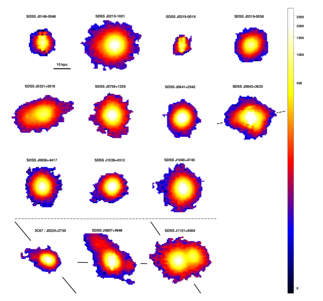
Figure 1: Intensity maps of the [O iii] line from the sample obscured quasars (11 radio-quiet and 3 radio-loud/radio-intermediate objects, separated by the dashed line), with a cutoff at a signal-to-noise ratio of 5, shown on a logarithmic color scale. The tick marks of the color bar are in units of $10^{-17}$ erg s^-1 cm^-2 arcsec^-2. All maps have the same spatial scale as shown in the top left panel. The orientation of the scattering axis for SDSS J0842+3625 (101^∘ east of north, Zakamska et al., 2005) is marked by thick dashed lines. The orientation of the jets from the radio objects is denoted by thick solid lines.

The average seeing of 0.4–0.7″ corresponds to a typical linear resolution of $\sim$3 kpc at the typical redshifts of our sample. In Figure 2 we show a detailed comparison of the [O iii] surface brightness profiles with the PSFs. We fit elliptical isophotes to the continuum-free [O iii] line intensity map of each object using the ellipse task from the IRAF STSDAS package. In the Figure, we show the surface brightness of each isophote as a function of both semi-major and semi-minor axes. The seeing is determined by averaging the directly measured FWHM of a sample of field stars in the acquisition image taken right before the science exposure. In Figure 2, each PSF is represented by the radial profile of our standard star whose width is scaled to match the seeing of each observation. The standard star is slightly elongated (ellipticity = 0.07), and here we conservatively use the profile along its major-axis. The radial profiles of our targets are clearly extended except SDSS J0841+2042 and SDSS J1039+4512. These two objects, although they appear only marginally resolved, demonstrate evident velocity gradient and [O iii] line width variation across their maps (which we will show in an upcoming paper) and a strong radial change of [O iii]/H$\beta$ line ratio similar to that seen in other objects (see Section 3.4). We thus conclude that all the quasar nebulae are spatially resolved by our IFU observations.

Figure 2: [O iii] surface brightness profiles of the quasars in our sample along both the semi-major axes of the best-fit isophotal ellipses (solid lines) and the semi-minor axes (dot-dash lines), compared to the profiles of continuum emission along the semi-major axes (dashed lines) and the PSF at the time of the observation (dotted lines). The peak [O iii] surface brightness ($I_{0}$) marked on each panel is in $10^{-14}$ erg s^-1 cm^-2 arcsec^-2. The continuum emission profiles are truncated at their respective 5–$\sigma$ levels. Also given in each panel is the absolute value of the best-fit exponent ($\eta$) of power-law fits to the outer regions of the nebulae along the semi-major axes (i.e., $I_{R,\rm[O~{}{\scriptscriptstyle III}]}\propto R^{-\eta}$).

3.2 Size Measurements

The physical size of a quasar’s narrow-line region is one of the basic parameters that characterize the impact of the active nucleus on its environment; yet this value is not an easy one to define. The options include (but are not limited to):

1. $R_{5\sigma}$, the radius of the best-fit ellipse which encloses pixels with a signal-to-noise ratio of 5 or higher. This measurement faithfully reports the observed extent of a quasar nebula, but the size depends on the depth that an observation reaches, making it difficult to compare objects observed with different sensitivity and/or at different redshifts.

2. $R_{\rm eff}$, the effective radius which encloses half of the total luminosity of the line emission. Due to the steep decline of the light profiles in the central parts, this approach has the advantage that $R_{\rm eff}$ is relatively insensitive to the detection threshold or to faint extended emission. However, this is also the disadvantage if faint extended emission is what we are after. Furthermore, since there is no universal surface brightness profile amongst quasar nebulae, $R_{\rm eff}$ does not provide a complete characterization of the nebula.

3. $R_{\rm obs}$, the isophotal radius at an observed limiting surface brightness of $10^{-16}$ erg s^-1 cm^-2 arcsec^-2. In this work, this threshold is chosen so that the measurements stay above $\sim 3\sigma$ sensitivity level for our sample objects. This definition may be useful for nearby objects in which cosmological dimming effects are negligible.

4. $R_{\rm int}$, the isophotal radius at an intrinsic limiting surface brightness of $10^{-15}$ erg s^-1 cm^-2 arcsec^-2, which is corrected by a factor of $(1+z)^{4}$ (ranging from 4.5 to 7.4 for our objects) in order to account for the cosmological surface brightness dimming effect. This threshold corresponds to a 6–$\sigma$ detection for the worst case in our sample. This relatively conservative threshold is a compromise between our data and the data with lower sensitivity and/or at higher redshifts which we take from the literature for various comparisons. $R_{\rm int}$ is better physically motivated than the previous measures, in that it does not depend on the depth of the observations and the redshifts of the objects.

All the above radii are defined as the semi-major axes of the best-fit ellipses at their respective isophotes or signal-to-noise ($S/N$) levels. The measured diameters of the ionized gas nebulae range from 15 to 40 kpc, as seen from the $R_{5\sigma}$ values determined from the [O iii] maps. Not just the faint extended gas envelopes, but the bright central parts are resolved by our observations: the effective radii are from 1.4 to 2.9 times the effective radii of the corresponding PSFs. All size measurements are reported in Table 2.

We also compute the ellipticities of the isophotes corresponding to the radii listed above. Ellipticities are defined as $\epsilon\equiv 1-b/a$ where $a$ and $b$ are the semi-major and semi-minor axis, respectively, and are reported in Table 2 except for ellipticities at $R_{\rm eff}$ which are affected by the PSF and are thus not reported. The nebulae of radio-quiet quasars are nearly round, with $\epsilon_{5\sigma}=0.13\pm 0.12$ (mean and standard deviation).

Furthermore, we create continuum maps for all objects by summing up the spectrum over a 200-300Å wavelength range where line features are absent and artifacts are minimal (typically either 4400–4700Å or 5200–5400Å), and perform differential photometry on these maps in the identical manner to that employed for [O iii] line images. We list both the $R_{5\sigma}^{\rm cont}$ and the $R_{\rm eff}^{\rm cont}$ in Table 2. Our sensitivity to the continuum observations is limited, since the continuum is extracted using a relatively narrow wavelength range; therefore, the continuum profiles shown in Figure 2 with dashed lines are truncated at much smaller distances from the center than the profiles of the nebular emission. The continua are spatially resolved, with $R_{\rm eff}^{\rm cont}$ ranging from 1.3 to 2.3 times the effective radii of the corresponding PSFs, and are nearly round for the radio-quiet quasars, with $\epsilon_{5\sigma}^{\rm cont}=0.14\pm 0.05$.

In Figure 3 we show the distribution of relative sizes and relative ellipticities for the nebulae and the continua. For radio-quiet objects, the ratio $R_{\rm eff}/R_{\rm eff}^{\rm cont}$ ranges between 0.90 and 1.33, with the mean and standard deviation of $1.11\pm 0.18$. The continuum is likely due to the combination of the starlight from the host galaxy and the small amount of light from the obscured quasar that escapes along unobscured directions, scatters off the interstellar medium of the galaxy and reaches the observer. Since scattered light is polarized, polarimetry or spectropolarimetry can provide a way to determine the dominant direction of quasar illumination (Antonucci & Miller, 1985; Tran et al., 1995; Zakamska et al., 2005, 2006). The contribution of the scattered light to the total continuum emission ranges from 0 to 60% (Liu et al., 2009). Thus the spatial profile of the continuum is determined by both the distribution of stars in the galaxy and the distribution of the interstellar medium, whereas the sizes of the emission line nebulae are determined by the distribution of the ionized gas.

The small ellipticities of the continuum emission suggest that the scattered light emission (which tends to show pronounced conical or biconical structure; Zakamska et al. 2006) is either not an important contributor or is concentrated close to the center of the galaxy on scales smaller than the seeing. Of the sources presented here, spectropolarimetric observations are available for SDSS J0842+3625. This object’s continuum emission is polarized at an astonishing 20% level, and there are no discernible stellar features in the deep optical spectrum we took of this source (Zakamska et al., 2005). These data indicate that much, if not most, of the continuum is due to the scattered light. The position angle of the E-vector of polarization is 11^∘ east of north and therefore the dominant illumination direction is 101^∘ east of north, as indicated in Figure 1 with dotted lines. Although some elongation of [O iii] emission is vaguely visible in this direction, the continuum morphology shows no features. Therefore, even in this rather extreme source the scattered light emission is not spatially resolved by the ground-based observations, and the combination of HST and polarimetric observations would be necessary to determine the relative importance of starlight and scattered light in our sample.

Since the narrow-line emission and the continuum are produced by different components of the galaxy via different emission mechanisms, the close similarity of the effective sizes of the nebulae and the continua is rather surprising. The key question is whether the warm ionized gas observed via its line emission is co-spatial with stars or whether the gas is in fact being pushed out of the galaxy by the quasar into the intergalactic medium. Therefore, the proper comparison would be not between the effective radii of the nebular and continuum emission, but rather between the density profiles of the ionized gas and the stars. We hope to be able to obtain the density profiles of the ionized gas by extending the range of our photo-ionization models of the kind presented in Section 4.4. To get accurate stellar light profiles would require HST-quality data to separate out the scattered light contribution (Zakamska et al., 2005, 2006).

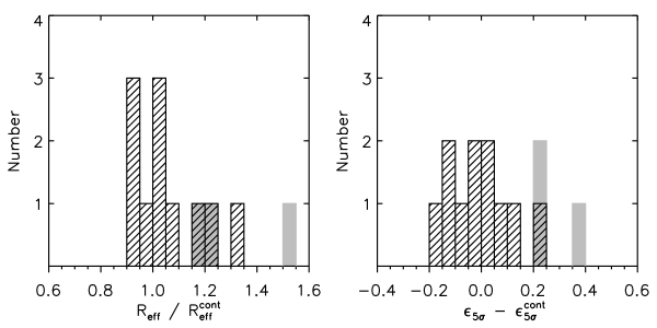
Figure 3: Comparison of the extents and ellipticities between the [O iii]$\lambda$5007 line and the continuum maps of our quasars. In the eleven radio-quiet objects (striped bars), the effective radii of the nebulae and the continua are similar, as are their ellipticities. The three radio-loud objects are represented by gray solid bars.

3.3 Size-Luminosity Relation

We now investigate the relationship between the integrated [O iii] luminosity and the size of the nebula – the size/luminosity relationship shown in Figure 4. In addition to our own data on the high-luminosity end of the diagram, we use several samples from the literature. These datasets include IFU maps of two type 2 quasars (Humphrey et al., 2010), long-slit spectroscopy of type 2 quasars at $z$=0.1–0.4 (Greene et al., 2011), and long-slit spectroscopy of nearby Seyfert 2 galaxies (Bennert et al., 2006; Fraquelli et al., 2003). HST narrow-band imaging campaigns (Schmitt et al., 2003; Bennert et al., 2002) are included in the figure (represented by gray symbols) but are not used in any quantitative measurements, because they are shallower than IFU and long-slit spectroscopy by 1–2 orders of magnitude and thus do not reach down to the surface brightness levels we use in our analysis (Greene et al., 2011).

Except for the solid gray symbols, the radius reported in Figure 4 is $R_{\rm int}$, the isophotal radius at $10^{-15}/(1+z)^{4}$ erg s^-1 cm^-2 arcsec^-2 which corrects the sizes for cosmological dimming and is thus the measure of choice for samples that include objects at different redshifts. For our data, we employ a conservative approach to estimate the uncertainty of $R_{\rm int}$. Taking into account that the SDSS calibration error is $\lesssim 10\%$ (Section 2.3), and that the isophote at $R_{\rm int}$ corresponds to a signal-to-noise ratio of 3.5–10.7 among the radio-quiet objects, we find a 10-30% uncertainty. This is an overestimate, because measuring an isophotal radius involves averaging many pixels and the uncertainty is thus suppressed; but the pixels are actually not independent and the uncertainty is difficult to further quantify. We budget a further 30% uncertainty to account for continuum subtraction and instrumental and pipeline errors, and combining all these uncertainties in quadrature leads to a final uncertainty of $\lesssim 40\%$ in our surface brightness measurements. Since the surface brightness declines as a steep function of radius, we find that the uncertainty in our determined $R_{\rm int}$ are about 5–14% for the eleven radio-quiet quasars.

We remeasure the radii of the targets in the four relevant studies (Fraquelli et al., 2003; Bennert et al., 2006; Humphrey et al., 2010; Greene et al., 2011) to determine $R_{\rm int}$ in a uniform manner to construct the size-luminosity relation. Among the six objects observed by Humphrey et al. (2010), only two radio-quiet quasars are resolved and found to be surrounded by ionized gas nebulae. We assign a 50% uncertainty for their radii, which is an arbitrary but conservative estimate from their IFU [O iii] maps with 1″ spaxels and 1.2″-1.6″ seeing. All the 15 quasars in the Greene et al. (2011) sample are measured using the 1-dimensional spatial profile of [O iii], and we adopt the uncertainty of about 50% estimated by Greene et al. (2011) to account for the unknown elongation of these nebulae.

For the objects in the Bennert et al. (2006) and Fraquelli et al. (2003) samples the cosmological dimming effect of surface brightness is not important because these Seyfert 2 galaxies are nearby (the most distant object CGCG 420-015 is at $z=0.0294$). Our limiting surface brightness level corresponds to $10^{33.7}$ erg s^-1 pc^-2 in their units for all these targets. Both groups have provided the best-fit power laws of the [O iii] surface brightness profiles, which we use to obtain $R_{\rm int}$ (the [O iii] profile of ESO 362–G008 is not available and we exclude this source from the sample of Bennert et al., 2006). For the two targets included in both samples, NGC 1386 and NGC 5643, we choose the profiles given in Bennert et al. (2006), because these authors subtract the contribution of the star formation to the ionization of [O iii]. We adopt the uncertainties estimated by Fraquelli et al. (2003) for their objects, while for the five Bennert et al. (2006) objects we propagate the uncertainties in the best-fit power indices to $R_{\rm int}$.

The uniformly defined sizes from previous investigations and the addition of our high-quality size measurements at high luminosity are combined into a single size-luminosity relationship in Figure 4. The $R_{\rm int}$ sizes are strongly correlated with [O iii] luminosity, and we fit the relationship with a power law. We perform a linear regression on the well-measured logarithmic data points, with upper limits and double continuum sources from Greene et al. (2011) excluded. We use linear regression algorithm linmix_err from the IDL Astronomy User’s Library, which applies a Bayesian approach using Markov chain Monte Carlo to calculate the posterior probabilities as described in Kelly (2007). By fitting a Gaussian profile to the resultant posterior distribution of the slope and intercept which are both close to normal distributions, we take advantage of Bayesian methods to reliably calculate the uncertainties. Assuming a 15% uncertainty for all $L_{\rm[O~{}{\scriptscriptstyle III}]}$ measurements, we find a best-fit linear relation

log($R_{\rm int}$/pc)=($0.250\pm 0.018$) log($L_{\rm[O~{}{\scriptscriptstyle III}]}/10^{42}$ erg s^-1)+($3.746\pm 0.028$).

The best-fit parameters are consistent within 1$\sigma$ with those found by Greene et al. (2011). In particular, we confirm the shallow slope they find ($0.22\pm 0.04$). We caution that the shallow slope hinges in part on the data points at the faint end from Fraquelli et al. (2003), which are based on extrapolations from their power-law fit to the [O iii] profile rather than real measurements (see also discussion in Husemann et al., 2012).

We detect extended [O iii] emission in every case, whereas Humphrey et al. (2010) conducted IFU observations of type 2 quasars drawn from the same parent sample (Zakamska et al., 2003; Reyes et al., 2008) and resolved two out of six objects. The most likely reasons for this difference are the smaller luminosity of the objects selected by Humphrey et al. (2010) (which implies smaller expected sizes, as per our size-luminosity diagram) and the 2–3 times better seeing of our observations.

Figure 4: Size-luminosity relation of the radio-quiet quasars in the [O iii] emission line from our sample (black solid diamonds), added to the previous observations including IFU mapping (Humphrey et al., 2010) and long-slit spectroscopy (Greene et al., 2011) of type 2 quasars at $z$=0.1–0.4, and long-slit spectroscopy of nearby Seyfert 2 galaxies (Bennert et al., 2006; Fraquelli et al., 2003). HST narrow-band imaging campaigns (Schmitt et al., 2003; Bennert et al., 2002) are shown with gray symbols but are not used in any quantitative analyses, because they are shallower than IFU and long-slit spectroscopy by about 1 to 2 orders of magnitude (Greene et al., 2011).

3.4 Emission line ratios

Among the various optical line ratios, [O iii]/H$\beta$ is one of the best diagnostics of the ionization mechanism (Baldwin et al., 1981; Veilleux & Osterbrock, 1987; Osterbrock & Ferland, 2006). In order to create the intensity maps of the H$\beta$ emission line, we first need to evaluate the contribution of the host galaxy. Unlike the case of [O iii] where a local linear continuum fit is sufficient, the measurement of H$\beta$ may be biased by the absorption lines in the stellar photospheres of the host galaxy. We take the fiber spectrum of each object from the SDSS database and decompose the continuum into a linear sum of the principle components derived from pure absorption-line galaxies (Hao et al., 2005). We subtract the best-fit host galaxy continuum from each SDSS spectrum and find that the H$\beta$ flux changes by no more than a few percent, with the exception of SDSS J0319-0019 (Figure 5). This object shows a strong post-starburst continuum (Goto et al., 2003), and subtraction of this component leads to a detection of H$\beta$ emission with a $S/N\sim 2.5$ at the peak of the line (which is otherwise undetected in the total spectrum). We attempted to apply this strategy to the IFU data of this target in a spatially resolved manner, but could not reliably recover the extended H$\beta$ emission, because the baseline determination is hindered by the chip gap in vicinity of the H$\beta$ line. Therefore, we do not perform spatially resolved analysis of [O iii]/H$\beta$ in this one target. In the remaining objects, we create the intensity maps of the H$\beta$ line emission from our sample objects in an identical manner as for the [O iii] line.

Figure 5: Spectra of our sample quasars, taken from the SDSS DR7 except for 3C67 whose spectrum is obtained by collapsing our Gemini IFU datacube along spatial dimensions. The original SDSS spectra have much broader wavelength coverage than the GMOS spectra examined in this paper, but do not contain any spatial information. The marked emission lines are: ($a$) [O ii] 3727Å; ($b$) [Ne iii] 3869Å; ($c$) [Ne iii] 3871Å; ($d$) H$\delta$ 4102Å; ($e$) H$\gamma$ 4341Å; ($f$) [O iii] 4363Å; ($g$) He ii 4686Å; ($h$) H$\beta$ 4861Å; ($i$) [O iii] 4959Å; ($j$) [O iii] 5007Å. Right panels show the velocity substructures in the [O iii] 5007Å line in the rest frame of the sources as determine using the redshifts listed in Table 1. The GMOS spectra analyzed in this paper typically cover He ii, H$\beta$ and [O iii].

To avoid oversampling within the PSF and to increase the $S/N$ ratio, we rebin the intensity maps so that the pixel size matches the full width at 1$\sigma$ of the Gaussian profile (i.e., pixel scale = 2$\sigma$) that represents the corresponding observational PSF. In Figure 6, the [O iii]/H$\beta$ line ratio is plotted against the [O iii] line surface brightness ($\Sigma_{\rm[O~{}{\scriptscriptstyle III}]}$) and the corresponding isophotal radius (semi-major axis from the elliptical differential photometry of the [O iii]$\lambda$5007 map, see Section 3.1). In this spatially resolved pixel-by-pixel analysis, we have only considered pixels with $S/N\geqslant 3$ in both lines. Although the three radio-loud and radio-intermediate quasars are included, their isophotal morphology is not as well represented by ellipses as radio-quiet objects, therefore the $\Sigma_{\rm[O~{}{\scriptscriptstyle III}]}$-to-radius conversion introduces larger uncertainties.

Figure 6 reveals a universal behavior of the [O iii]/H$\beta$ line ratio in our entire sample of radio-quiet quasars: the ratio persists at a constant value of roughly 10 in the central regions, until it reaches a “break” isophotal radius ranging from $\sim$4.1 to 11 kpc where it starts to decrease. In Section 4.4 we further discuss this figure and present our qualitative interpretation of this behavior.

In addition to H$\beta$ and [O iii] we detect several weaker emission lines. Because of their lower total fluxes, they are typically detected out to smaller distances than H$\beta$ (and of course smaller yet than [O iii]). One of these, He ii $\lambda$4686Å, turns out to be diagnostic of physical conditions in the nebula. We describe the underlying physics and present the He ii $\lambda$4686Å measurements in Section 4.4.

The wavelength coverage of the GMOS spectra is rather limited, and H$\gamma$ is covered only in a couple of objects in the region of poor filter transmission. The typical reddening of the narrow-line regions of type 2 quasars was estimated by (Reyes et al., 2008) from the spatially integrated SDSS spectra to be $A_{V}=1.0-2.6$ mag based on the observed H$\alpha$/H$\beta$ and H$\beta$/H$\gamma$ ratios. The only two line ratios we are discussing in the present paper are [O iii]/H$\beta$ and He ii/H$\beta$. Because all these lines are close together in wavelength, de-reddening would result in a small correction to these ratios of $\lesssim 0.06$ dex.

Figure 6: [O iii]/H$\beta$ as a function of [O iii] surface brightness and isophotal radius (semi-major axis). For each object, we list the [O iii]/H$\beta$ ratio on the plateau (labeled “const”), the [O iii] surface brightness and radius where the break occurs, and the best-fit power-law slope of the non-plateau regimes for each object are marked. The breaks are depicted by dotted lines.

Figure 7: Continued.

4 Discussion

4.1 Comparison with radio-loud objects

We find extended ($\gtrsim$ 20 kpc-scale) ionized gas nebula in every highly luminous radio-quiet obscured quasar that we have examined at $z\sim 0.5$. This finding is in contrast to many previous studies, beginning with Stockton & MacKenty (1987), which found few if any radio-quiet objects with extended line emission; rather, it was the radio-loud quasars that routinely displayed powerful extended emission-line regions. Since we are now able to extend previous studies to a higher quasar luminosity, particularly for obscured quasars, we revisit the comparison between the properties of the nebulae of radio-loud and radio-quiet objects.

Jets are frequently implicated in strong interactions with galactic interstellar matter (Oosterloo et al., 2000), in exciting the gas through shocks (Cecil et al., 2001) and in producing outflows of gas from the host galaxy, often on scales of several kpc (Baum et al., 1990, 1992; McCarthy, 1993; Morganti et al., 2005; Nesvadba et al., 2006). At high redshifts, the emission-line regions can be extended over tens of kpc, contain significant amounts of mass and are typically well-aligned with the large-scale jet emission (Nesvadba et al., 2006, 2008). At low redshifts, there is no particularly strong alignment between the jet and the emission-line gas (Privon et al., 2008), perhaps with marginal evidence for alignment in younger radio sources still confined to their host galaxy. The lack of alignment could have many explanations – for example, the pattern of quasar illumination of the interstellar medium may be different from the jet direction, or inhomogeneities in the gas could lead to nebulae expanding in the directions of lowest density. No obvious alignment is seen in the three radio-loud sources we observed as part of our campaign (bottom of Fig. 1). Of the four extended emission features seen in our three radio-loud sources, only one feature in SDSS J0807+4946 lies along its radio axis.

For comparison with our objects, an ideal radio-loud sample would contain type 2 sources (i.e., radio galaxies) with similar redshifts and [O iii] luminosities observed to similar depth. Narrow-band imaging data from space (e.g., for 3C objects, Tremblay et al., 2009) are therefore not a good option because they are shallower than our IFU data by 1–2 orders of magnitude. A close-to-optimal sample was studied by Fu & Stockton (2009) who consider eight radio-loud sources. Their objects are type 1 radio-loud quasars which are a bit closer than ours ($z=0.16-0.37$) and have slightly lower luminosities ($L_{\rm[O~{}{\scriptscriptstyle III}]}=10^{42\mathchar 45\relax 43}$ erg s^-1), but their IFU data is very well matched to our observations.

The most striking difference between our radio-quiet objects and the radio-loud sources studied by Fu & Stockton (2009) is that the objects from the latter sample show much more complex morphologies in their [O iii] emission. The nebulae studied by Fu & Stockton (2009) often consist of several kinematically and/or morphologically separate clumps and blobs, and even when the emission is connected into a single nebula it is not a linear structure that we could fit with an ellipse for comparison with our observations. Fu & Stockton (2009) suggest that the blobs and clumps could be due to quasar-illuminated merger debris or the remnants of a quasar-driven wind.

In view of the limited availability of comparison radio-loud objects at low redshifts, we consider high-redshift samples as well. We construct the radio-loud comparison sample by combining the three radio-loud quasars in our own Gemini campaign (Fig. 1, bottom three) with three powerful radio galaxies MRC 0316-257, MRC 0406-244 and TXS 0828+193. These three objects, located at $z\sim$2–3, were observed with SINFONI in the IFU mode on the VLT by Nesvadba et al. (2008). The isophotal radii $R_{\rm int}$ (semi-major axes) and ellipticities $\epsilon_{\rm int}$ are measured the same way as for radio-quiet quasars at the [O iii] surface brightness of 10^-15 erg s^-1 cm^-2 arcsec^-2 (i.e., corrected for cosmological dimming). These results, along with some basic information about the three high-redshift objects, are listed in Table 3.

In Figure 8, we show the radii $R_{\rm int}$ and ellipticities $\epsilon_{\rm int}$ of the eleven radio-quiet and the six radio-loud quasars plotted against their radio luminosity at 1.4 GHz. The 1.4 GHz fluxes are taken from the FIRST survey for SDSS objects and the NRAO/VLA Sky Survey (NVSS, Condon et al., 1998) for the rest and are then used to calculate the rest-frame-corrected monochromatic luminosities at 1.4 GHz (Zakamska et al., 2004). In the case of non-detections in the FIRST survey, we report the upper limits for a point source (5$\sigma$+0.25 mJy, Collinge et al., 2005).

Separated by the vertical dotted line at $\nu L_{\nu}[1.4{\rm GHz}]=1.1\times 10^{41}$ erg s^-1 (our adopted radio-quiet/radio-loud criterion discussed in Section 2.1), the nebulae of the two populations of quasars demonstrate an evident difference in their ellipticities. All the radio-loud objects have elongated narrow-line nebulae with $\epsilon_{\rm int}>0.25$, while ten out of eleven radio-quiet quasars have $\epsilon_{\rm int}<0.25$, with SDSS J0321+0016 being the only exception. In terms of their respective mean value and standard deviation, the ellipticities of radio-quiet quasars have $\epsilon_{\rm int}=0.16\pm 0.10$, while their radio-loud peers have $\epsilon_{\rm int}=0.45\pm 0.14$. The most striking morphological difference between the ionized gas nebulae around radio-loud and radio-quiet objects is that the radio-quiet ones are significantly rounder. In contrast, the [O iii] line emission from all the three objects in Nesvadba et al. (2008) are remarkably elongated along the direction of their radio jets.

The semi-major axes of radio-loud nebulae ($R_{\rm int}=19.9\pm 6.9$ kpc) are larger than those of radio-quiet objects ($11.1\pm 3.0$ kpc), although the difference in sizes is not as dramatic as it is for ellipticities and there is some overlap in the size distributions. It is perhaps the larger sizes and larger ellipticities of the nebulae in radio-loud objects that made them more easily detectable in previous studies.

Our radio-loud / radio-quiet criterion is set at $\nu L_{\nu}[1.4~{}{\rm GHz}]=1.1\times 10^{41}$ erg s^-1, which is a negligible fraction of the bolometric luminosity, but could correspond to a significant mechanical energy of the jet. For example, applying equations of Cavagnolo et al. (2010) we find that an $L_{\rm mech}=5\times 10^{44}$ erg s^-1 jet could be hiding behind this rather small radio luminosity. It is precisely the dramatic difference in morphology and ellipticity of the ionized gas nebulae that occurs at roughly this radio luminosity that leads us to conclude that jets are not an important contributor to supplying and exciting ionized gas in our eleven radio-quiet sources.

4.2 Comparison with Unobscured Quasars

Another natural comparison is between our sample and unobscured radio-quiet quasars at similar luminosities and redshifts. Among the existing studies, the sample of Husemann et al. (2008) and (Husemann et al., 2012) is fairly well matched to ours in luminosity, although their sources are at slightly lower redshifts ($z<0.3$). At similar surface brightness limits, those authors do not find the spatially extended round nebulae that we see in our radio-quiet sample of type 2 quasars. They find extended [O iii] emission in 61% of the objects in their sample (the rest are non-detections). Compared to our objects, their nebulae appear elongated and/or irregular (with ellipticities range from 0.15 to 0.64), and there is a trend for targets with high Fe ii equivalent width (the doublet $\lambda\lambda$4924,5018 plus the complex at 5100–5405Å) and low H$\beta$ FWHM to have smaller nebulae. This last issue is not testable with our data because the Fe ii emitting regions are obscured in our targets. These authors also find that the extended nebulae are aligned with the radio jets even when the jets are weak, and that the size of the nebulae increases for increasing radio luminosity.

One of the possible explanations for the difference between the detection rate of nebulae in our sample and in that by Husemann et al. (2008) is that by selecting sources with high [O iii] equivalent width (as is the case in our sample) we are preferentially selecting those with high covering factor in O²⁺ (Baskin & Laor, 2005; Ludwig et al., 2009). Furthermore, despite the careful subtraction of the bright PSF (the quasar itself), faint emission on the scales of the host galaxy may be difficult to see in type 1 quasars, and thus the detected nebulae may be biased toward those that are larger and more elongated. Finally, geometric effects of quasar illumination may play a role: since type 2 quasars are obscured along the line of sight, the illumination of the gas may be happening on average closer to the plane of the sky than it does in type 1 quasars, thus producing apparently larger nebulae.

Alternatively, the difference in the morphology of ionized gas around type 1 and type 2 quasars may reflect an actual evolutionary difference between the two types. Theoretical models of galaxy formation have long postulated an evolutionary scenario in which galaxy mergers induce both star formation and nuclear activity, triggering a transition from an obscured accretion and star formation stage (more likely to be seen as a type 2 source) to an unobscured phase as a type 1 quasar (e.g., Sanders et al., 1988). A variety of observational studies support a scenario of this type, finding for example that host galaxies of type 2 active galactic nuclei exhibit more star formation than do the hosts of type 1’s (Ho, 2005; Lacy et al., 2007; Zakamska et al., 2008). Thus it is plausible that obscured quasars are more likely to be seen with extended ionized emission because they are in fact associated with a phase in which gas is being expelled out from the galaxy (Hopkins et al., 2006).

4.3 Comparison with Seyfert galaxies and the origin of gas

Schmitt et al. (2003) compiled and analyzed HST narrow-band imaging data on [O iii] nebulae in a large sample of Seyfert 1 and Seyfert 2 galaxies. The typical r.m.s. surface brightness limit of their observations is $1.2\times 10^{-15}$ erg s^-1 cm^-2 arcsec^-2, so these data probe the bright central regions of the targets on scales of a few hundred parsecs at typical resolutions of $\sim$50 pc. The median [O iii] luminosity of the Seyfert galaxies in this sample is 2.5 dex smaller than the median [O iii] luminosities of the quasars in our sample.

Taking just the 38 type 2 Seyfert galaxies from this sample, we find that the ellipticities of their nebulae are distributed between 0.06 and 0.75, with the mean of 0.42. Many objects show pronounced biconical structures in their [O iii] emission lines. Furthermore, we find 10 objects with position angles of the [O iii] nebulae $\theta_{\rm[O~{}{\scriptscriptstyle III}]}$ measured by Schmitt et al. (2003) for which polarization position angles $\theta_{\rm pol}$ are available in the literature (as referenced in Schmitt et al. 2003). The average difference between the two sets of angles is $\langle|\Delta\theta|\rangle=97^{\circ}\pm 6^{\circ}$. This value is in strong disagreement with that expected if $\theta_{\rm[O~{}{\scriptscriptstyle III}]}$ and $\theta_{\rm pol}$ were each independently drawn from a uniform distribution between $0^{\circ}$ and $180^{\circ}$, in which case the probability distribution of $|\Delta\theta|$ would be $p(\Delta\theta)\propto(1-|\Delta\theta|/180^{\circ})$ and would be peaked at small angles.

As was already discussed in Section 3.2, the polarization is produced when light from the hidden nucleus is scattered off of the extended material, and the illumination direction (as projected on the plane of the sky) is orthogonal to the measured polarization angle. Thus, in Seyfert 2 galaxies [O iii] nebulae are not only elongated, but are closely aligned with the illumination direction. Both the scattered light and the [O iii] emission are produced along the directions of clear view toward the nucleus, and in the classical model of toroidal obscuration (Antonucci & Miller, 1985) one expects to see ionization bicones – as indeed observed in the sample of Schmitt et al. (2003).

In our sample, the observed morphologies of the nebulae are determined both by the gas distribution in and around the host galaxy and by the illumination pattern of the quasar. The lack of elongation or biconical structures either in the morphology of the ionized gas or in the continuum tracing the dominant quasar illumination directions is one of the major surprises of our observations. One possible explanation is that the typical opening angles of quasar illumination are large, producing quasi-isotropic illumination pattern. Another possibility is that at the high luminosities explored in this paper the geometry of obscuration is different from that seen in Seyfert galaxies: perhaps there is no organized toroidal structure, but rather obscuration is quasi-spherical and patchy, so that ionizing emission escapes along random beams (but not toward the observer) which we cannot spatially resolve by our data. Both these possibilities are at odds with our HST imaging of somewhat less luminous type 2 quasars which clearly shows ionization cones in at least some objects (Zakamska et al., 2006), although a strong luminosity dependence of the geometry of obscuration would reconcile these results. HST imaging of the objects in this sample in the blue band sensitive to the scattered light emission can settle this issue.

An alternative possibility is that shock excitation rather than photo-ionization is responsible for the observed strong line emission. The radiation pressure of the quasar (Murray et al., 1995; Proga et al., 2000) drives a low-density high-temperature wind (Faucher-Giguère & Quataert, 2012; Zubovas & King, 2012) which slams into dense clumps in the host galaxy, resulting in shocked emission. Numerical simulations demonstrate that even if there are anisotropies in the initial driving of the outflow, the outflow isotropizes over the range of scales involved between the scale on which the outflow is accelerated ($\lesssim 10$ pc) and the scale on which it sweeps up the interstellar medium of the galaxy ($\sim 10$ kpc), producing structures qualitatively similar to those seen in our observations (Novak et al., 2011). Shocks propagating at several hundred km s^-1 normally do not produce [O iii]/H$\beta\sim 10$ (Rich et al., 2011) as seen in our quasars, and thus they are normally disfavored as the primary origin of narrow line emission. Furthermore, the efficiency of converting mechanical energy into line emission is expected to be low at such shock velocities (Nesvadba et al., 2008). One possibility is that the shock blast propagates much faster ($>1000$ km s^-1) than was previously considered, resulting in higher [O iii]/H$\beta$ ratios consistent with those observed. Thus, we will continue to explore this possibility in our future work since photo-ionization does not at the moment provide a fully satisfactory explanation of all of the aspects of our data.

Figure 8: Sizes and ellipticities ($R_{\rm int}$ and $\epsilon_{\rm int}$, see Section 3.2 for their definition) of the [O iii] nebulae around 11 radio-quiet quasars from our observations, compared to those of the six radio-loud objects (Table 3). The comparison sample of six contains three low-redshift radio galaxies from our own observations and three high-redshift radio galaxies from Nesvadba et al. (2008).

4.4 Physical conditions in the nebulae

In this Section we discuss a plausible model of a nebula under the assumption that the gas is illuminated and photo-ionized in a wide-angle manner, either because of the large opening angles in the obscuring material or because of the quasi-spherical patchy illumination. Unless noted otherwise, the arguments in this section apply both to a static nebula and to an outflow. Throughout this section we use $r$ to denote the three-dimensional distance from the quasar and $R$ to denote the distance as seen projected onto the plane of the sky.

We aim to determine plausible physical conditions for the line-emitting gas that we observe. Regardless of the mechanism by which the gas reached the observed radii, it is reasonable to draw an analogy with galaxy-scale winds, in which there is also observed warm line-emitting gas at large radii. In these cases, the gas is multi-phase, with different phases of the medium observable in different domains of the electromagnetic spectrum. By analogy with the winds driven by supernova explosions in star-burst galaxies (Heckman et al., 1990; Veilleux et al., 2005), the simplest model involves two components. One consists of hot, low-density, volume-filling potentially X-ray-emitting plasma, whereas the other is warm ($T\sim 10^{4}$ K), higher density component concentrated in clumps, shells or filaments (hereafter “clouds”). It is the latter that produces the emission lines that we see in optical spectra. If the two components are in rough pressure equilibrium with each other, their densities and temperatures are related via $n_{\rm hot}T_{\rm hot}\simeq n_{\rm warm}T_{\rm warm}$.

The [O iii]/H$\beta$ ratio shows a remarkably uniform behavior as a function of distance from the center across our sample. As Figure 6 demonstrates, for all the radio and radio-quiet objects that we observe (except for SDSS J0319-0019 where we have only a weak detection of H$\beta$), the ratio remains constant at [O iii]/H$\beta=12.3\pm 2.7$ out to distances of $7.0\pm 1.8$ kpc, and declines as $\log$ [O iii]/H$\beta\propto R^{-3.3\pm 1.1}$ at larger distances. In addition, most objects show a characteristic excess ($\sim$0.2 dex) of [O iii]/H$\beta$ right at about the break radius.

We consider two physically distinct models that can qualitatively account for the behavior of the line ratios. The first model capitalizes on the fact that the [O iii]/H$\beta$ ratio is strongly dependent on the ionization parameter $U\equiv\Phi/4\pi cr^{2}n_{\rm H}(r)$, where $\Phi$ is the photon luminosity of the quasar above the ionization energy of hydrogen of 13.6 eV. Following Villar-Martín et al. 2008, we consider a simple case of clouds of constant density $n_{\rm H}=100$ cm^-3 illuminated by a quasar with bolometric luminosity $L_{\rm bol}=10^{46}$ erg s^-1. In this model, for a typical quasar spectral energy distribution (Ferland et al., 1998) the ionization parameter as a function of distance is $\log U=-0.87-\log(r/{\rm kpc})^{2}$. We then use calculations presented in Villar-Martín et al. 2008 to determine the [O iii]/H$\beta$ ratios of such clouds (Figure 9, left panel labeled “Model 1”). As long as the clouds remain “ionization-bounded” at all distances from the quasar (i.e., the number of O²⁺-ionizing photons is insufficient to ionize the entire cloud) and the value of $U$ stays above $\log U\simeq-2.3$, the [O iii]/H$\beta$ ratio is constant and close to 10. As $r$ increases and $U$ declines below $\log U\simeq-2.3$, the [O iii]/H$\beta$ ratio declines as well, in qualitative agreement with our observations.

Despite the apparent success of this model in reproducing the [O iii]/H$\beta$ ratio, the input physics is not entirely satisfactory. In particular, since the clouds’ thermal balance is maintained by photo-ionization and recombination, their temperatures are nearly constant under a wide range of conditions with $T=f\times 10^{4}$ K where the factor $f$ is typically between 1 and 2 (Krolik, 1999). Since the model assumes a constant density inside the clouds, this implies that the cloud pressure is independent of the distance from the quasar as well. If the clouds are in pressure equilibrium with the confining low-density medium, this would imply that the pressure of the entire quasar nebula is constant as a function of radius. This is hard to reconcile with models, as well as with observations of starburst-driven winds in which pressure declines outwards (Heckman et al., 1990).

Therefore, we consider another simple model in which the pressure in the nebula follows $P(r)\propto r^{-2}$. The clouds are in confined by the pressure of the hot low-density component, and since their temperature is almost constant, the density inside them drops as $n_{\rm H}(r)\propto r^{-2}$ as well, which implies that the ionization parameter is independent of the distance from the quasar. We use the photo-ionization code Cloudy (Ferland et al., 1998) to model emission of clouds with a hydrogen density of $n=100$ cm^-3 at $r=1$ kpc from a $L_{\rm bol}=10^{46}$ erg s^-1 quasar. These parameters correspond to an ionization parameter of $\log U=-0.87$.

In Figure 9, center, we show the [O iii]/H$\beta$ ratios of such clouds as a function of their physical depth. Large clouds are ionization-bounded (i.e., have a large optical depth) and show the familiar ratio of [O iii]/H$\beta\simeq 10$. Smaller clouds, however, allow for the photons with energies above 54.9 eV (the energy required to ionize O²⁺ into O³⁺) to penetrate through the entire cloud, destroying most O²⁺ ions and resulting in much lower [O iii]/H$\beta$ ratios. If a cloud is participating in the outflow, it expands (linear size $S\propto r^{2/3}$), its density falls ($\propto r^{-2}$) and its optical depth declines ($\propto r^{-4/3}$). Therefore, as the clouds propagate out with the quasar wind, they are expected to transition from ionization-bounded (partly ionized) to matter-bounded (fully ionized). The same transition occurs in a static nebula as long as clouds have the same mass distribution at all distances. As a result, the [O iii]/H$\beta$ ratio is expected to fall as a function of distance from the quasar, in qualitative agreement with our observations.

All the arguments presented thus far apply equally to a static nebula or a wind, as long as the pressure profiles are similar. We now consider specifically an outflowing wind. In the matter-bounded regime the H$\beta$ luminosity of each cloud $L_{\rm cloud}\propto n^{2}S^{3}\propto r^{-2}$. If the number density of clouds falls off as $r^{-2}$ (as expected in a steady-state constant velocity wind), then the H$\beta$ luminosity density falls off as $r^{-4}$. As a result, the surface brightness of the nebula is expected to fall off as $R^{-3}$, which is close to the values seen in our sample (Table 2, the mean value of the exponent is $-3.5\pm 1.0$).

The major difference between Models 1 and 2 is in the degree of ionization of clouds at large distances from the quasar. In Model 1, the ionization parameter decreases outward and the clouds have a smaller degree of ionization than they do in the inner parts. In Model 2, the hard radiation can penetrate through the entire cloud, ionizing O²⁺ to higher ionization states. Coincidentally, the ionization energy of O²⁺ (54.9 eV) is almost identical to the ionization energy of He⁺ (54.4 eV). Thus the same photons that destroy O²⁺ and lead to the decrease of the [O iii]/H$\beta$ ratio in Model 2 produce He²⁺. This leads to an increase in He²⁺ recombination emission, including one of the transitions in the recombination cascade observed as the optical line He ii $\lambda$4686Å. Thus, Model 2 predicts a much higher ratio of He ii/H$\beta$ in the outer parts in the nebula than does Model 1. The model predictions are illustrated in Figure 9, right. The models do not take into account projection effects – along any given line of sight, regions at different distance $r$ from the quasar contribute to the emission. Nevertheless, it is clear that high He ii/H$\beta$ ratios, especially in combination with low [O iii]/H$\beta$, are characteristic of the high-ionization matter-bounded regions and can only be produced in Model 2.

In Figure 10 we present the measurements of the He ii/H$\beta$ line ratios in the 10 sources where the He ii $\lambda$4686Å transition is covered by our data. The He ii line is weaker than H$\beta$ and is thus cannot be measured out to the same distances from the quasar, although typically we are able to detect He ii at distances comparable to or larger than the break radius. There is a general tendency for He ii/H$\beta$ ratio to increase outward, and in 9/10 objects it goes above $\log$ [He ii/H$\beta$]=$-0.5$ – too high to be compatible with Model 1. The key upper left region of the He ii/H$\beta$ vs [O iii]/H$\beta$ diagnostic diagrams is particularly observationally difficult because it is reached only in the outermost parts of the nebulae where [O iii] is faint; nevertheless, the line ratios in two objects – SDSS J0210$-$1001 and SDSS J0842$+$3625 – extend into this region.

We will continue to refine Models 1 and 2 as we investigate other aspects of our data. From the simple model setup presented above, we conclude that the pressure in the nebulae is most likely decreasing outward and that line-emitting clouds transition from ionization-bounded to matter-bounded as the distance from the quasar increases.

Figure 9: Left: In the model where all clouds are ionization-bounded and have the same density ($n_{\rm H}=100$ cm^-3), the [O iii]/H$\beta$ ratio shows a behavior qualitatively similar to that observed in our sources (plotted here as a function of three-dimensional distance $r$). Center: A model with declining pressure profile uses the fact that the [O iii]/H$\beta$ ratio changes dramatically as the clouds transition from being ionization-bounded to matter-bounded. Here, we show the [O iii]/H$\beta$ ratios of clouds of varying thickness at a distance of 1 kpc from a $10^{46}$ erg s^-1 quasar calculated with Cloudy. Right: The two models predict similar [O iii]/H$\beta$ behavior as a function of distance, but different He ii/H$\beta$ ratios (Model 1 shown with dashed line, Model 2 shown with solid line).

Figure 10: He ii/H$\beta$ as a function of [O iii] isophotal radius (left panels) and [O iii]/H$\beta$. Large values of He ii/H$\beta$ ($\log$ He ii/H$\beta\gtrsim-0.5$) strongly suggest presence of matter-bounded clouds, especially in combination with low [O iii]/H$\beta$ ($\log$ [O iii]/H$\beta\lesssim 0.5$), as seen in SDSS J0210$-$1001 and SDSS J0842$+$3625.

Figure 11: Continued.

5 Conclusions

In this paper we present optical seeing-limited integral field unit observations of ionized gas around $z\simeq 0.5$ obscured luminous quasars. We use these data to determine the spatial distribution of the [O iii]$\lambda$5007Å and H$\beta$ line emission. We spatially resolve the emission line nebulae in every case and find that the [O iii] line emission from gas photo-ionized by the hidden quasar is detected out to $14\pm 4$ kpc from the center of the galaxy (sample mean and standard deviation are given throughout this section). Ionized gas nebulae around radio-quiet obscured quasars display regular smooth morphologies, in marked contrast with nebulae around radio-loud quasars of similar line luminosities which tend to be significantly more elongated and/or lumpy. Surprisingly, no pronounced biconical structures expected in a simple quasar illumination model are detected.

The main measurements we present in this paper are (1) the spatial distribution of the emission-line surface brightness, (2) the spatial distribution of the [O iii]/H$\beta$ ratios, and (3) the relationship between the size of the nebula and the emission line luminosity. When fit to a power law, the surface brightness of H$\beta$ declines as $R^{-3.5\pm 1.0}$ as a function of the distance from the quasar, whereas [O iii] surface brightness declines as $R^{-3.8\pm 0.7}$. The [O iii]/H$\beta$ ratios show a remarkably uniform behavior across the sample: the ratio remains constant at $12.3\pm 2.7$ and at $R\gtrsim 7\pm 2$ kpc declines as roughly a power-law function of the distance from the quasar with an index $-3.3\pm 1.1$. Finally, we supplement our sample with 31 objects in the literature, define a redshift- and sensitivity-independent nebula size and present a size-luminosity relationship uniformly measured over six orders of magnitude in line luminosity. The nebular size slowly increases with luminosity $\propto L^{0.250\pm 0.018}$.

The galaxy-wide narrow-line emission regions around our quasars are large, but the origin of this ionized gas is unclear. In principle, the quasar may be illuminating previously existing gas in the galaxy halo (e.g. from previous star formation, Steidel et al., 2010); or the gas may be debris associated with recent merger activity and currently illuminated by the quasar (see, e.g. Fu & Stockton, 2009; Stockton et al., 2006). The remarkable roundness of the nebulae and the lack of distinct blobs or clumps is in direct contrast to the morphologies seen in radio-loud objects (c.f. Fu et al., 2011). It is hard to understand how tidal debris or gas accretion could leave such a smooth and isotropic distribution of gas. One option is that the gas is being expelled from the galaxy, presumably driven by the radiative pressure of the quasar itself (Murray et al., 1995; Proga et al., 2000). We cannot rule out that previous generations of star formation have left behind the gas now illuminated by the quasar, but we do note that the smooth featureless morphologies of the [O iii] nebulae in our sample are similar to those seen in wide-angle outflows recently observed by Rupke & Veilleux (2011).

We put forward a simple model of a clumpy gaseous nebula, in which the lower density hotter component is largely invisible, but the higher-density warm component is the one we observe via line emission. In our fiducial model, the gas pressure inside the nebula and in the clouds drops off as $r^{-2}$ and the temperature of the emission-line clouds is nearly constant at a few $\times 10^{4}$ K determined by the photo-ionization and emission balance. The clouds closer to the quasar are denser and are ionization-bounded (i.e., the photo-ionizing photons from the quasar are all absorbed on the quasar-facing side of the cloud and cannot penetrate all the way), whereas the clouds beyond $r\gtrsim 7$ kpc are lower-density, larger and matter-bounded (i.e., the recombination rate cannot keep up with the ionization rate, and these clouds are fully ionized). Unlike the model with a constant pressure profile, the model with a declining pressure profile qualitatively explains our [O iii]/H$\beta$ and He ii/H$\beta$ line ratio observations and the surface brightness distributions, and will be tested and refined further by our on-going observations and modeling.

The kinematic analysis of extended line emission around quasars is on-going and will be presented in our upcoming papers. We will demonstrate that the nebulae whose morphological properties are discussed here are likely due to ionized gas in the outflow from the quasar. If these outflows are found to carry significant kinetic energy and/or momentum ($\sim 1\%$ of the bolometric output of the quasar), they will be excellent candidates for the long-sought feedback phase of quasar evolution.

Table 1: Properties of our Gemini quasar sample.

Object name	Radio	$f_{\rm 1.4GHz}$	$z$	PA	$t_{\rm exp}$	Seeing	$\log L_{\rm[OIII]}$	$\delta L/L$	$\eta$
(1)	(2)	(3)	(4)	(5)	(6)	(7)	(8)	(9)	(10)
SDSS J014932.53$-$004803.7	RQ	1.03	0.566	323	1800$\times$2	0.52	42.87	0.13	5.70$\pm$0.14
SDSS J021047.01$-$100152.9	RQ	$<$1.20	0.540	280	1800$\times$2	0.58	43.48	0.10	3.00$\pm$0.02
SDSS J031909.61$-$001916.7	RQ	1.95	0.635	273	1800$\times$2	0.38	42.74	0.16	3.00$\pm$0.20
SDSS J031950.54$-$005850.6	RQ	$<$0.97	0.626	220	1800$\times$2	0.58	42.96	0.11	4.30$\pm$0.11
SDSS J032144.11$+$001638.2	RQ	1.58	0.643	150	1800$\times$2	0.54	43.10	0.11	3.02$\pm$0.08
SDSS J075944.64$+$133945.8	RQ	1.82	0.649	164	1800$\times$2	0.61	43.38	0.08	3.39$\pm$0.02
SDSS J084130.78$+$204220.5	RQ	$<$0.95	0.641	250	1800$\times$2	0.52	43.31	0.10	3.84$\pm$0.02
SDSS J084234.94$+$362503.1	RQ	1.64	0.561	0	1800$\times$2	0.46	43.56	0.14	3.93$\pm$0.02
SDSS J085829.59$+$441734.7	RQ	$<$0.90	0.454	55	1800$\times$2	0.60	43.30	0.06	4.06$\pm$0.02
SDSS J103927.19$+$451215.4	RQ	2.13	0.579	90	1800$\times$2	0.58	43.29	0.13	4.00$\pm$0.02
SDSS J104014.43$+$474554.8	RQ	4.28	0.486	10	1800$\times$2	0.74	43.52	0.09	3.53$\pm$0.01
3C67/J022412.30$+$275011.5	RL	3024	0.311	264	1800$\times$2	0.52	42.83	0.25	3.38$\pm$0.06
SDSS J080754.50$+$494627.6	RL	169.2	0.575	152	1800$\times$2	0.63	43.27	0.16	3.49$\pm$0.19
SDSS J110140.54$+$400422.9	RI	17.38	0.457	77	1800$\times$1	0.63	43.55	0.09	4.64$\pm$0.12

• Notes. – (1) object name. (2) Radio loudness (RQ: radio quiet; RL: radio loud; RI: radio intermediate). (3) Radio flux at 1.4 GHz in mJy, taken from the FIRST survey (Becker et al., 1995; White et al., 1997) and the NVSS survey (Condon et al., 1998, for 3C67 only). Upper limits are reported for undetected sources (see text). (4) Redshift, from Zakamska et al. (2003) and Reyes et al. (2008) for SDSS objects and Eracleous & Halpern (2004) for 3C67. (5) Position angle of the field of view (in degrees), measured by the shorter axis from north to east. (6) Exposure time (in seconds) and number of exposures. (7) Seeing at the observing site (FWHM, in arcseconds). (8) Total luminosity of the [O iii]$\lambda$5007Å line (erg s^-1), derived from our data calibrated against SDSS spectra, except for 3C67 whose [O iii] flux is taken from Gelderman & Whittle (1994). (9) Relative uncertainty of the [O iii] luminosity. The uncertainty for 3C67 is taken from Gelderman & Whittle (1994). (10) Absolute value of the best-fit power-law exponent of the outer part of the [O iii] profile along the major axes (i.e., $I_{R,{\rm[OIII]}}\propto R^{-\eta}$, see Figure 2).

Table 2: Properties of our Gemini quasar sample (continued).

Object	$R_{5\sigma}^{\rm cont}$	$\epsilon_{5\sigma}^{\rm cont}$	$R_{5\sigma}$	$\epsilon_{5\sigma}$	$R_{\rm eff}^{\rm cont}$	$R_{\rm eff}$	$R_{\rm obs}$	$\epsilon_{\rm obs}$	$R_{\rm int}$	$\epsilon_{\rm int}$	const	$R_{\rm br}$	slope	$\zeta$
(1)	(2)	(3)	(4)	(5)	(6)	(7)	(8)	(9)	(10)	(11)	(12)	(13)	(14)	(15)
SDSS J0149$-$0048	6.3	0.06	9.1	0.10	3.1	2.9	7.4	0.12	6.9	0.05	31.8	4.1	$-$4.79$\pm$0.37	3.27$\pm$0.11
SDSS J0210$-$1001	4.8	0.21	17.7	0.07	3.0	4.0	17.8	0.14	14.4	0.12	10.0	7.5	$-$3.09$\pm$0.22	2.08$\pm$0.14
SDSS J0319$-$0019	9.9	0.13	7.6	0.25	3.0	2.7	7.9	0.22	6.7	0.23	—	—	—	—
SDSS J0319$-$0058	5.5	0.16	11.5	0.04	3.3	3.5	11.2	0.05	9.6	0.14	11.9	7.5	$-$5.32$\pm$1.34	4.64$\pm$0.22
SDSS J0321$+$0016	8.2	0.17	18.3	0.42	4.3	5.2	19.3	0.38	16.6	0.42	16.2	11.0	$-$2.66$\pm$0.35	5.02$\pm$0.23
SDSS J0759$+$1339	6.0	0.22	14.1	0.02	3.0	3.5	15.4	0.07	12.9	0.08	16.1	7.5	$-$2.91$\pm$0.31	3.06$\pm$0.08
SDSS J0841$+$2042	5.5	0.07	11.9	0.09	2.8	2.5	11.8	0.10	10.0	0.17	15.7	6.4	$-$3.53$\pm$0.28	3.65$\pm$0.08
SDSS J0842$+$3625	6.5	0.17	15.1	0.12	3.1	3.2	14.4	0.18	13.1	0.19	10.3	9.0	$-$4.14$\pm$0.56	4.82$\pm$0.19
SDSS J0858$+$4417	6.9	0.12	11.7	0.08	3.0	3.1	11.5	0.12	10.6	0.10	11.9	5.6	$-$3.88$\pm$1.16	3.24$\pm$0.16
SDSS J1039$+$4512	4.9	0.19	12.2	0.24	2.5	2.6	11.4	0.22	9.3	0.12	12.2	5.8	$-$3.90$\pm$0.65	4.54$\pm$0.14
SDSS J1040$+$4745	6.9	0.09	14.5	0.04	3.6	3.4	14.5	0.08	13.0	0.18	8.7	7.6	$-$2.45$\pm$0.75	2.88$\pm$0.20
3C67/J0224$+$2750	5.2	0.07	12.2	0.42	2.0	2.3	19.4	0.42	10.1	0.26	4.6	8.3	$-$2.38$\pm$0.90	2.99$\pm$0.18
SDSS J0807$+$4946	5.8	0.22	19.4	0.44	2.7	3.3	19.2	0.47	14.6	0.45	13.8	6.3	$-$1.45$\pm$0.45	3.60$\pm$0.04
SDSS J1101$+$4004	4.7	0.05	18.9	0.26	3.4	5.2	19.3	0.31	18.7	0.31	12.3	8.2	$-$2.90$\pm$0.36	2.16$\pm$0.03

• Notes. – (1) object name. (2–3) Semi-major axis (in kpc) and ellipticity ($\equiv 1-b/a$) of the best-fit ellipse which encloses pixels with $S/N\geqslant 5$ in the continuum map. (4–5) Semi-major axis (in kpc) and ellipticity of the best-fit ellipse which encloses pixels with $S/N\geqslant 5$ in the [O iii]$\lambda$5007Å line map. (6–7) Half-light isophotal radius (effective radius) of the continuum and [O iii]$\lambda$5007Å line emission (semi-major axis, in kpc). (8–9) Isophotal radius (semi-major axis, in kpc) and ellipticity at the observed limiting surface brightness of $10^{-16}$ erg s^-1 cm^-2 arcsec^-2. (10–11) Isophotal radius (semi-major axis, in kpc) and ellipticity at the intrinsic limiting surface brightness (corrected for cosmological dimming) of $10^{-15}$ erg s^-1 cm^-2 arcsec^-2. (12) Mean value of the plateau part of the [O iii]/H$\beta$ radial profile. (13) Break radius (semi-major axis) of the [O iii]/H$\beta$ radial profile. (14) Best-fit power-law slope of the [O iii]/H$\beta$ radial profile at $R>R_{\rm br}$. (15) Absolute value of the best-fit power-law exponent of the H$\beta$ radial profile at $R>R_{\rm br}$ (i.e., $I_{R,{\rm H\beta}}\propto R^{-\zeta}$).

Table 3: Properties of the radio galaxies from Nesvadba et al. (2008).

Object name	Type	$f_{\rm 1.4GHz}$	$z$	Seeing	$\log L_{\rm[O~{}{\scriptscriptstyle III}]}$	$R_{\rm eff}$	$\epsilon_{\rm eff}$	$R_{\rm int}$	$\epsilon_{\rm int}$
		(mJy)		(″)	(erg s-1)	(kpc)		(kpc)
MRC 0316–257	RL	447	3.127	0.7$\times$0.4	44.29	4.3	0.37	21.27	0.59
MRC 0406–244	RL	626	2.425	0.7$\times$0.6	44.50	4.6	0.43	28.12	0.48
TXS 0828+193	RL	118	2.577	0.7$\times$0.5	44.51	6.6	0.56	26.66	0.61

• Notes. – All notations are identical to Table 1 and 2. Redshift (determined from the [O iii]$\lambda$5007Å line), seeing and [O iii] luminosity data are taken from Nesvadba et al. (2008). Radio fluxes are from the NVSS survey (Condon et al., 1998).

References

- Abazajian et al. (2009) Abazajian, K. N., Adelman-McCarthy, J. K., Agüeros, M. A., et al. 2009, ApJS, 182, 543
- Allington-Smith et al. (2002) Allington-Smith, J., Murray, G., Content, R., et al. 2002, PASP, 114, 892
- Antonucci (1993) Antonucci, R. 1993, ARA&A, 31, 473
- Antonucci & Miller (1985) Antonucci, R. R. J., & Miller, J. S. 1985, ApJ, 297, 621
- Arav et al. (2008) Arav, N., Moe, M., Costantini, E., et al. 2008, ApJ, 681, 954
- Baldwin et al. (1981) Baldwin, J. A., Phillips, M. M., & Terlevich, R. 1981, PASP, 93, 5
- Baskin & Laor (2005) Baskin, A., & Laor, A. 2005, MNRAS, 358, 1043
- Baum et al. (1990) Baum, S. A., Heckman, T., & van Breugel, W. 1990, ApJS, 74, 389
- Baum et al. (1992) Baum, S. A., Heckman, T. M., & van Breugel, W. 1992, ApJ, 389, 208
- Becker et al. (1991) Becker, R. H., White, R. L., & Edwards, A. L. 1991, ApJS, 75, 1
- Becker et al. (1995) Becker, R. H., White, R. L., & Helfand, D. J. 1995, ApJ, 450, 559
- Bennert et al. (2002) Bennert, N., Falcke, H., Schulz, H., Wilson, A. S., & Wills, B. J. 2002, ApJ, 574, L105
- Bennert et al. (2006) Bennert, N., Jungwiert, B., Komossa, S., Haas, M., & Chini, R. 2006, A&A, 456, 953
- Boroson et al. (1985) Boroson, T. A., Persson, S. E., & Oke, J. B. 1985, ApJ, 293, 120
- Cavagnolo et al. (2010) Cavagnolo, K. W., McNamara, B. R., Nulsen, P. E. J., et al. 2010, ApJ, 720, 1066
- Cecil et al. (2001) Cecil, G., Bland-Hawthorn, J., Veilleux, S., & Filippenko, A. V. 2001, ApJ, 555, 338
- Collinge et al. (2005) Collinge, M. J., Strauss, M. A., Hall, P. B., et al. 2005, AJ, 129, 2542
- Condon et al. (1998) Condon, J. J., Cotton, W. D., Greisen, E. W., et al. 1998, AJ, 115, 1693
- Crenshaw et al. (2003) Crenshaw, D. M., Kraemer, S. B., & George, I. M. 2003, ARA&A, 41, 117
- Croton et al. (2006) Croton, D. J., et al. 2006, MNRAS, 365, 11
- Donahue et al. (2006) Donahue, M., Horner, D. J., Cavagnolo, K. W., & Voit, G. M. 2006, ApJ, 643, 730
- Dunn et al. (2010) Dunn, J. P., Bautista, M., Arav, N., et al. 2010, ApJ, 709, 611
- Eracleous & Halpern (2004) Eracleous, M., & Halpern, J. P. 2004, ApJS, 150, 181
- Fanaroff & Riley (1974) Fanaroff, B. L., & Riley, J. M. 1974, MNRAS, 167, 31P
- Faucher-Giguère & Quataert (2012) Faucher-Giguère, C.-A., & Quataert, E. 2012, MNRAS, 425, 605
- Ferland et al. (1998) Ferland, G. J., Korista, K. T., Verner, D. A., et al. 1998, PASP, 110, 761
- Ferrarese & Merritt (2000) Ferrarese, L., & Merritt, D. 2000, ApJ, 539, L9
- Fraquelli et al. (2003) Fraquelli, H. A., Storchi-Bergmann, T., & Levenson, N. A. 2003, MNRAS, 341, 449
- Fu et al. (2011) Fu, H., Myers, A. D., Djorgovski, S. G., & Yan, L. 2011, ApJ, 733, 103
- Fu & Stockton (2009) Fu, H., & Stockton, A. 2009, ApJ, 690, 953
- Gallagher et al. (2007) Gallagher, S. C., Hines, D. C., Blaylock, M., et al. 2007, ApJ, 665, 157
- Ganguly & Brotherton (2008) Ganguly, R., & Brotherton, M. S. 2008, ApJ, 672, 102
- Gebhardt et al. (2000) Gebhardt, K., et al. 2000, ApJ, 539, L13
- Gelderman & Whittle (1994) Gelderman, R., & Whittle, M. 1994, ApJS, 91, 491
- Goto et al. (2003) Goto, T., Nichol, R. C., Okamura, S., et al. 2003, PASJ, 55, 771
- Greene et al. (2011) Greene, J. E., Zakamska, N. L., Ho, L. C., & Barth, A. J. 2011, ApJ, 732, 9
- Greene et al. (2012) Greene, J. E., Zakamska, N. L., & Smith, P. S. 2012, ApJ, 746, 86
- Gültekin et al. (2009) Gültekin, K., et al. 2009, ApJ, 698, 198
- Hao et al. (2005) Hao, L., Strauss, M. A., Fan, X., et al. 2005, AJ, 129, 1795
- Häring & Rix (2004) Häring, N., & Rix, H.-W. 2004, ApJ, 604, L89
- Heckman et al. (1990) Heckman, T. M., Armus, L., & Miley, G. K. 1990, ApJS, 74, 833
- Ho (2005) Ho, L. C. 2005, preprint (astroph/0511157)
- Hopkins et al. (2006) Hopkins, P. F., Hernquist, L., Cox, T. J., et al. 2006, ApJS, 163, 1
- Humphrey et al. (2010) Humphrey, A., Villar-Martín, M., Sánchez, S. F., et al. 2010, MNRAS, L113
- Husemann et al. (2008) Husemann, B., Wisotzki, L., Sánchez, S. F., & Jahnke, K. 2008, A&A, 488, 145
- Husemann et al. (2012) —. 2012, ArXiv e-prints
- Jia et al. (2012) Jia, J., Ptak, A., Heckman, T., & Zakamska, N. 2012, ArXiv e-prints
- Jiang et al. (2007) Jiang, L., Fan, X., Vestergaard, M., et al. 2007, AJ, 134, 1150
- Kelly (2007) Kelly, B. C. 2007, ApJ, 665, 1489
- Krolik (1999) Krolik, J. H. 1999, Active galactic nuclei : from the central black hole to the galactic environment (Princeton, NJ: Princeton University Press)
- Lacy et al. (2007) Lacy, M., Sajina, A., Petric, A. O., et al. 2007, ApJ, 669, L61
- Lal & Ho (2010) Lal, D. V., & Ho, L. C. 2010, AJ, 139, 1089
- Liu et al. (2009) Liu, X., Zakamska, N. L., Greene, J. E., et al. 2009, ApJ, 702, 1098
- Ludwig et al. (2009) Ludwig, R. R., Wills, B., Greene, J. E., & Robinson, E. L. 2009, ApJ, 706, 995
- Magorrian et al. (1998) Magorrian, J., Tremaine, S., Richstone, D., et al. 1998, AJ, 115, 2285
- Marconi & Hunt (2003) Marconi, A., & Hunt, L. K. 2003, ApJ, 589, L21
- McCarthy (1993) McCarthy, P. J. 1993, ARA&A, 31, 639
- McConnell et al. (2011) McConnell, N. J., Ma, C.-P., Gebhardt, K., et al. 2011, Nature, 480, 215
- McNamara & Nulsen (2007) McNamara, B. R., & Nulsen, P. E. J. 2007, ARA&A, 45, 117
- Moe et al. (2009) Moe, M., Arav, N., Bautista, M. A., & Korista, K. T. 2009, ApJ, 706, 525
- Morganti et al. (2005) Morganti, R., Tadhunter, C. N., & Oosterloo, T. A. 2005, A&A, 444, L9
- Murray et al. (1995) Murray, N., Chiang, J., Grossman, S. A., & Voit, G. M. 1995, ApJ, 451, 498
- Nesvadba et al. (2008) Nesvadba, N. P. H., Lehnert, M. D., De Breuck, C., Gilbert, A. M., & van Breugel, W. 2008, A&A, 491, 407
- Nesvadba et al. (2006) Nesvadba, N. P. H., Lehnert, M. D., Eisenhauer, F., et al. 2006, ApJ, 650, 693
- Novak et al. (2011) Novak, G. S., Ostriker, J. P., & Ciotti, L. 2011, ApJ, 737, 26
- O’Dea et al. (2002) O’Dea, C. P., de Vries, W. H., Koekemoer, A. M., et al. 2002, AJ, 123, 2333
- Oosterloo et al. (2000) Oosterloo, T. A., Morganti, R., Tzioumis, A., et al. 2000, AJ, 119, 2085
- Osterbrock & Ferland (2006) Osterbrock, D. E., & Ferland, G. J. 2006, Astrophysics of gaseous nebulae and active galactic nuclei (Sausalito, CA: University Science Books)
- Privon et al. (2008) Privon, G. C., O’Dea, C. P., Baum, S. A., et al. 2008, ApJS, 175, 423
- Proga et al. (2000) Proga, D., Stone, J. M., & Kallman, T. R. 2000, ApJ, 543, 686
- Ptak et al. (2006) Ptak, A., Zakamska, N. L., Strauss, M. A., et al. 2006, ApJ, 637, 147
- Randall et al. (2011) Randall, S. W., Forman, W. R., Giacintucci, S., et al. 2011, ApJ, 726, 86
- Reichard et al. (2003) Reichard, T. A., et al. 2003, AJ, 125, 1711
- Reyes et al. (2008) Reyes, R., Zakamska, N. L., Strauss, M. A., et al. 2008, AJ, 136, 2373
- Rich et al. (2011) Rich, J. A., Kewley, L. J., & Dopita, M. A. 2011, ApJ, 734, 87
- Rupke & Veilleux (2011) Rupke, D. S. N., & Veilleux, S. 2011, ApJ, 729, L27
- Sanders et al. (1988) Sanders, D. B., Soifer, B. T., Elias, J. H., et al. 1988, ApJ, 325, 74
- Scannapieco & Oh (2004) Scannapieco, E., & Oh, S. P. 2004, ApJ, 608, 62
- Schmitt et al. (2003) Schmitt, H. R., Donley, J. L., Antonucci, R. R. J., et al. 2003, ApJ, 597, 768
- Shen et al. (2008) Shen, Y., Greene, J. E., Strauss, M. A., Richards, G. T., & Schneider, D. P. 2008, ApJ, 680, 169
- Silk & Rees (1998) Silk, J., & Rees, M. J. 1998, A&A, 331, L1
- Spinelli et al. (2006) Spinelli, P. F., Storchi-Bergmann, T., Brandt, C. H., & Calzetti, D. 2006, ApJS, 166, 498
- Springel et al. (2005) Springel, V., Di Matteo, T., & Hernquist, L. 2005, MNRAS, 361, 776
- Steidel et al. (2010) Steidel, C. C., Erb, D. K., Shapley, A. E., et al. 2010, ApJ, 717, 289
- Stockton et al. (2006) Stockton, A., Fu, H., Henry, J. P., & Canalizo, G. 2006, ApJ, 638, 635
- Stockton & MacKenty (1987) Stockton, A., & MacKenty, J. W. 1987, ApJ, 316, 584
- Tabor & Binney (1993) Tabor, G., & Binney, J. 1993, MNRAS, 263, 323
- Tadhunter (1991) Tadhunter, C. N. 1991, MNRAS, 251, 46P
- Tchekhovskoy et al. (2010) Tchekhovskoy, A., Narayan, R., & McKinney, J. C. 2010, ApJ, 711, 50
- Thoul & Weinberg (1995) Thoul, A. A., & Weinberg, D. H. 1995, ApJ, 442, 480
- Tran et al. (1995) Tran, H. D., Cohen, M. H., & Goodrich, R. W. 1995, AJ, 110, 2597
- Tremaine et al. (2002) Tremaine, S., et al. 2002, ApJ, 574, 740
- Tremblay et al. (2009) Tremblay, G. R., Chiaberge, M., Sparks, W. B., et al. 2009, ApJS, 183, 278
- van Breugel et al. (1986) van Breugel, W. J. M., Heckman, T. M., Miley, G. K., & Filippenko, A. V. 1986, ApJ, 311, 58
- van Dokkum (2001) van Dokkum, P. G. 2001, PASP, 113, 1420
- Veilleux et al. (2005) Veilleux, S., Cecil, G., & Bland-Hawthorn, J. 2005, ARA&A, 43, 769
- Veilleux & Osterbrock (1987) Veilleux, S., & Osterbrock, D. E. 1987, ApJS, 63, 295
- Vignali et al. (2010) Vignali, C., Alexander, D. M., Gilli, R., & Pozzi, F. 2010, MNRAS, 404, 48
- Villar-Martín et al. (2011a) Villar-Martín, M., Humphrey, A., Delgado, R. G., Colina, L., & Arribas, S. 2011a, MNRAS, 418, 2032
- Villar-Martín et al. (2008) Villar-Martín, M., Humphrey, A., Martínez-Sansigre, A., et al. 2008, MNRAS, 390, 218
- Villar-Martín et al. (2011b) Villar-Martín, M., Tadhunter, C., Humphrey, A., et al. 2011b, MNRAS, 416, 262
- Villar-Martín et al. (1999) Villar-Martín, M., Tadhunter, C., Morganti, R., Axon, D., & Koekemoer, A. 1999, MNRAS, 307, 24
- Voit (2005) Voit, G. M. 2005, Reviews of Modern Physics, 77, 207
- Voit & Donahue (2005) Voit, G. M., & Donahue, M. 2005, ApJ, 634, 955
- Weymann et al. (1981) Weymann, R. J., Carswell, R. F., & Smith, M. G. 1981, ARA&A, 19, 41
- White et al. (1997) White, R. L., Becker, R. H., Helfand, D. J., & Gregg, M. D. 1997, ApJ, 475, 479
- Whittle (1992) Whittle, M. 1992, ApJS, 79, 49
- Xu et al. (1999) Xu, C., Livio, M., & Baum, S. 1999, AJ, 118, 1169
- York et al. (2000) York, D. G., et al. 2000, AJ, 120, 1579
- Zakamska et al. (2008) Zakamska, N. L., Gómez, L., Strauss, M. A., & Krolik, J. H. 2008, AJ, 136, 1607
- Zakamska et al. (2004) Zakamska, N. L., Strauss, M. A., Heckman, T. M., Ivezić, Ž., & Krolik, J. H. 2004, AJ, 128, 1002
- Zakamska et al. (2003) Zakamska, N. L., et al. 2003, AJ, 126, 2125
- Zakamska et al. (2005) —. 2005, AJ, 129, 1212
- Zakamska et al. (2006) —. 2006, AJ, 132, 1496
- Zubovas & King (2012) Zubovas, K., & King, A. 2012, ApJ, 745, L34