Properties of the electron-positron plasma created from vacuum in a strong laser field. Quasiparticle excitations

Abstract

Solutions of a kinetic equation are investigated which describe, on a nonperturbative basis, the vacuum creation of quasiparticle electron-positron pairs due to a strong laser field. The dependence of the quasiparticle electron (positron) distribution function and the particle number density is explored in a wide range of the laser radiation parameters, i.e., the wavelength $\lambda$ and amplitude of electric field strength $E_{0}$. Three domains are found: the domain of vacuum polarization effects where the density of the $e^{-}e^{+}$ pairs is small (the “calm valley”), and two accumulation domains in which the production rate of the $e^{-}e^{+}$ pairs is strongly increased and the $e^{-}e^{+}$ pair density can reach a significant value (the short wave length domain and the strong field one). In particular, the obtained results point to a complicated short-distance electromagnetic structure of the physical vacuum in the domain of short wavelengths $\lambda\lesssim\lambda_{\rm acc}=\pi/m$. For moderately strong fields $E_{0}\lesssim E_{c}=m^{2}/e$, the accumulation regime can be realized where a plasma with a high density of $e^{-}e^{+}$ quasiparticles can be achieved. In this domain of the field strengths and in the whole investigated range of wavelengths, an observation of the dynamical Schwinger effect can be facilitated.

I Introduction

In the present work we investigate the response of the physical vacuum (PV) of QED to the influence of a time dependent, strong periodic electric field (”laser field”) in a wide range of field parameters, i.e., the field strength amplitude $E_{0}$ and the wavelength $\lambda$ (we use the natural units $\hbar=c=k_{B}=1$, $k_{B}$ being the Boltzmann constant),

$$0\leq E_{0}\lesssim E_{c}=m^{2}/e,$$ (1)

$$\pi/m=\pi\hskip 2.84526pt\vspace{2mm}\bar{}\vspace{-2mm}\lambda_{C}=\lambda_{\rm acc}\lesssim\lambda\leq\lambda_{0},$$ (2)

where $E_{c}$ is the so-called critical or Sauter-Schwinger field strength, and $\lambda_{C}=2\pi\hskip 2.84526pt\vspace{2mm}\bar{}\vspace{-2mm}\lambda_{C}$ is the Compton wavelength of elementary leptons with mass $m$ and electric charge $e=|e|$ (we focus here on electrons and positrons); $\lambda_{0}\sim 1~{}\mu$m . To characterize the PV response we use either the distribution function or the number density of quasiparticle electron-positron pairs (EPPs) created from the PV. Below we select three characteristic domains in the plane spanned by $E_{0}$ and $\lambda$: the region of non-increasing creation (dubbed ”calm valley”) and two boundary regions of accumulation, where the EPP density increases up to saturation (for sufficient duration of the field). The accumulation regions correspond to limiting high fields $E_{0}\sim E_{c}$ (and $\lambda\gg\lambda_{C}$) or limiting short wavelengths $\lambda\sim\lambda_{C}$ (and $E_{0}<E_{c}$). Of course, there is also a region where these accumulation domains do overlap. Different mechanisms of vacuum creation act in these domains and provide the corresponding features of the PV response. The vacuum excitations in the calm valley can be described perturbatively while nonperturbative approaches are necessary in both accumulation domains. In the following, we consider the action of a periodical field. But the obtained results allow also to estimate the role of separate Fourier components of an external field with complicated spectral structure (as, e.g., in the cases of vacuum EPP creation by scattering of charged particles at high energies Baur:2007df and the dynamical Casimir effect Dodonov:2010zza ).

The methodical basis of our analysis is a system of kinetic equations (KEs) which is a nonperturbative consequence of QED in the presence of a spatially homogeneous, time dependent electric field Kluger:1992 ; Schmidt:1998vi ; Pervushin:2006vh . These KEs are intended for the description of the dynamical Schwinger effect of vacuum particle creation in terms of quasiparticle vacuum excitations, having the quantum numbers of the electron and positron in the presence of an external field (mass, charge, quasi-momentum and quasi-energy), which are called below as quasiparticles. After the ceasing of the laser pulse some of these quasiparticles become real electrons and positrons with their momentum and energy lying on the mass shell.

Thus, in the present work, vacuum polarization effects and vacuum particle creation in the time-dependent electric field of a standing wave formed in the focal spot of counter-propagating strong laser fields are analyzed in the framework of the quasiparticle representation. Such a quasiparticle picture corresponds to the level of description with real EPPs in the out-channel. On the other hand, the information about quasiparticle distributions is useful for different estimates of the secondary observable effects such as the generation of pair annihilation photons Blaschke:2005hs ; Blaschke:2009uy ; Blaschke:2010vs ; Smolyansky:2010as ; Blaschke:2011af ; Blaschke:2011is , the birefringence effect (e.g., DiPiazza:2006pr ) and so on. The additional investigation of the residual EPP surviving after the ceasing of the laser pulse will be given elsewhere.

The present work is organized as follows. In Sect. II the basic KE and the set of limitations for their applicability are presented. The results of numerical investigations of the vacuum EPP creation kinetics for the case of a linearly polarized laser field are discussed in Sect. III for different domains of the external field parameters in the ranges (1) and (2). In the calm valley of the laser radiation parameters, the same results can be reproduced analytically in the low density approximation by using the peculiar perturbation theory (see Sect. IV). The summary of the results is given and discussed in Sect. V. Here the actuality of development of a nonperturbative kinetic theory of vacuum EPP creation for the case of non-quasiclassical external electromagnetic fields is emphasized for cases where the quantum field fluctuations are essential. It is also shown that both accumulation domains are promising for an experimental observation of the dynamical Schwinger effect.

II Basic kinetic equations

It is well known that vacuum particle creation in strong electromagnetic fields is possible if one or both of the field invariants $I_{1}=E^{2}-H^{2}$ and $I_{2}={\vec{E}}{\vec{H}}$ are non-vanishing Sauter:1931zz ; Heisenberg:1935qt ; Schwinger:1951nm ; Greiner:1985ce ; Grib:1994 . Such conditions can be realized, e.g., in the focal spot of two or more counter-propagating laser beams, where the electric field is spatially homogeneous over distances $\sim\lambda$ and time dependent. For very strong fields $E_{0}\sim E_{c}$ one can then expect the creation of a real electron-positron plasma Grib:1994 ; Brezin:1970xf ; Bulanov:2004de ; Narozhny:2006 ; Fedotov:2006 out of the electromagnetically polarized PV. In the subcritical field regime $E_{0}\ll E_{c}$ the question is mainly about the creation of a short-lived quasiparticle EPP that exists during the course of the field action (the dynamical Schwinger effect) Blaschke:2008wf ; Blaschke:2005hs . The possibilities for observing this kind of PV response with the help of secondary effects such as the radiation of annihilation photons are investigated intensively at the present time.

In this work, we study the PV response to a periodic model laser pulse with linear polarization $A^{\mu}(t)=(0,0,0,A(t))$ (Hamiltonian gauge), where

$$A(t)=(E_{0}/\nu)\cos(\nu t),\quad E(t)=E_{0}\sin(\nu t)~{}.$$ (3)

We are going to investigate the PV response as a function of the angular frequency $\nu=2\pi/\lambda$ (or the wavelength $\lambda$) and the amplitude $E_{0}$. For this aim we use the exact nonperturbative KE of the non-Markovian type for the one-body EPP phase-space distribution function $f(\mathbf{p},t)$ obtained in Schmidt:1998vi ,

$$\dot{f}(\mathbf{p},t)=\Lambda(\mathbf{p},t)\int^{t}_{0}dt^{\prime}\Lambda(\mathbf{p},t^{\prime})[\frac{1}{2}-f(\mathbf{p},t^{\prime})]\cos 2\theta(t,t^{\prime}),$$ (4)

where

$$\Lambda(\mathbf{p},t)=eE(t)\varepsilon_{\bot}/\omega^{2}(\mathbf{p},t)$$ (5)

is the amplitude of the EPP excitations with the quasi-energy $\omega(\mathbf{p},t)=\sqrt{\varepsilon^{2}_{\bot}(\mathbf{p})+(p_{\parallel}-eA(t))^{2}}$ and $\varepsilon_{\bot}=(m^{2}+p^{2}_{\bot})^{1/2}$ as the transverse energy; the quantity

$$\theta(t,t^{\prime})=\int^{t}_{t^{\prime}}d\tau\ \omega(\mathbf{p},\tau)$$ (6)

is the high frequency phase. The distribution function in the quasiparticle representation is defined relative to the in-vacuum state, $f(\mathbf{p},t)=\langle in\mid a^{+}(\mathbf{p},t)a(\mathbf{p},t)\mid in\rangle$, where $a(\mathbf{p},t)$ and $a^{+}(\mathbf{p},t)$ are the annihilation and creation operators in the quasiparticle representation. The existence of the quasi-energy $\omega(\mathbf{p},t)$ suggests that the quasiparticle excitations are not on the mass shell. For the generalization of the KE (4) to arbitrary electric field polarization, see Refs. Pervushin:2006vh ; Filatov:2006 ; Filatov:2009xd .

The KE (4) is equivalent to the system of ordinary differential equations

$$\dot{f} = \frac{1}{2}\Lambda u,$$

$$\dot{u} = \Lambda(1-2f)-2\omega v,$$ (7)

$$\dot{v} = 2\omega u,$$

which is convenient for the subsequent numerical investigations. The functions $u(\mathbf{p},t)$, $v(\mathbf{p},t)$ describe the vacuum polarization effects. Initial conditions at $t=0$ are $f=u=v=0$.

It is assumed that the laser electric field $E(t)$ (3) is quasiclassical. This means that the photon number with the frequency $\nu=2\pi/\lambda$ must be rather large in a volume of the order $\lambda^{3}$. This condition is fulfilled Berestetskii ; Ritus:1979 for

$$E_{0}\gg(\nu/2\pi)^{2}~{},$$ (8)

i.e., in the quasiclassical (QC) domain. In the quantum (Q) domain for $E_{0}\lesssim(\nu/2\pi)^{2}$ it is necessary to take into account the quantum fluctuations of the external electromagnetic field and a corresponding generalization of the KE (4) is required.

Below it will be shown that the features in the behavior of the PV response for the weak field case $E_{0}\ll E_{c}$ become apparent just in the Q domain, where the applicability of KE (4) breaks down. An exception is the strong field domain $E_{0}\lesssim E_{c}$, where the inequality (8) is valid. However, in spite of this, we will investigate its solutions here assuming that the external field can be treated as some quasiclassical background. Thus, these extrapolated solutions have the character of a preliminary forecast.

The adiabaticity parameter Popov:2001 ; Popov:2004 ; Delone:1998

$$\gamma=\frac{E_{c}}{E_{0}}\frac{\lambda_{c}}{\lambda}$$ (9)

is introduced for separating the domains of influence of two mechanisms of vacuum particle creation: tunneling for $\gamma\ll 1$ and multiphoton for $\gamma\gg 1$ processes. The point $\gamma=1$ corresponds to the boundary curve $E_{c}\lambda_{c}=E_{0}\lambda$ in Fig. 1 in the vicinity of which, however, no clear separation of these domains is possible.

It is assumed that the field (3) is switched on at $t_{0}=0$ (we ignore here the error brought in by such an instantaneous switching-on Grib:1994 ; Blaschke:2010sgu ). This way of switching on the external periodical field is rather standard in the framework of the discussed problem Grib:1994 ; Brezin:1970xf . Below we will consider also the method of adiabatic field switching on. Generally speaking, the obtained results depend on the way of the field switching on. This is due to the occurrence of high harmonics in the solution spectrum of the KE (4). As a rule, the high harmonics, which accompany the fast (non-adiabatic) switching on of a laser field, have no essential influence on the solution spectrum.

For a comparative investigation of EPP production as a function of the field parameters $\lambda$ and $E_{0}$ it is convenient to use some indicator characteristics. For this purpose we introduce here the maximal EPP number density $n_{\rm max}=n(t=T/4)$ which is related to the maximal distribution function $f_{\rm max}(\mathbf{p})=f(\mathbf{p},t=T/4)$ obtained from solving the KE (4) by integration over the momentum space

$$n(t)=g\int\frac{d^{3}p}{(2\pi)^{3}}f(\mathbf{p},t)~{},$$ (10)

where $g=4$ is the degeneracy factor, taking into account the spin and charge degrees of freedom. This definition is used below in the case of absence of accumulation effects for which the number density EPP grows rapidly. In Fig. 1 the above discussion is summarized in the “landscape” of the laser parameters $E_{0}$ and $\lambda$.

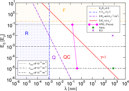
Figure 1: (Color online) Electron-positron pair production in the “landscape” of field strength $E_{0}$ and wavelength $\lambda$ of laser collider experiments, with a few examples for comparison (XFEL Ringwald:2001ib , Astra Gregori:2010uf , ELI Korzhimanov:2011 ). The hatched areas show the regions of accumulation due to the strong field (F) or resonance (R) mechanisms, resp. The black lines (dotted, dash-dotted, dash-double dotted) show three examples for peak pair densities $n_{\rm max}$. The violet dashed line depicts the limit between the quantum (Q) and the quasiclassical (QC) domain which itself is limited by the red solid line (adiabaticity index $\gamma=1$).

III Short-distance electromagnetic structure of the PV

A numerical investigation of the KE (4) demonstrates the complicated behavior of the distribution function which shows a series of qualitative modifications where the laser radiation parameters $E_{0}$ and $\lambda$ are varied in the boundaries (1) and (2). It is important to note that the character of the distribution function evolution depends strongly on the selection of the momentum representation: $f(\textbf{p},t)$ accomplishes some oscillations swinging along the $p_{\parallel}$ axis (the direction of the field (3)) as a whole with the amplitude $1/\gamma$ simultaneously with the ”breathing” mode, when its amplitude and form are altered. The transition to the kinematic momentum eliminates these oscillations and keeps the ”breathing” mode only.

The characteristic domains of dynamical behavior of the distribution function $f(\textbf{p},t)$ and the number density of EPPs (10) in the full range of the laser radiation parameters (1) and (2) are shown in Fig. 1 to be discussed step by step in what follows. The region outside the hatched accumulation domains due to strong field (F) and resonance (R) mechanisms of pair production is the calm valley. The boundary between quasiclassical (QC) and quantum (Q) domains of the electric field (3) is given by $E_{0}=1/\lambda^{2}$ and the line $\gamma=1$ separates the multiphoton and tunneling domains. Surprisingly, $n_{\rm max}$ is $\lambda$ independent practically in the whole calm valley, i.e. outside the accumulation domains R and F. Its dependence on the strength of electric field $E_{0}$ is shown in Fig. 2. The symbols on Fig. 1 depict also the basic parameters in the focal spot of the existing Liesfeld:2005 ; Gregori:2010uf and planned Ringwald:2001ib ; DiPiazza:2011tq ; Korzhimanov:2011 laser systems as, e.g., Astra, XFEL and ELI.

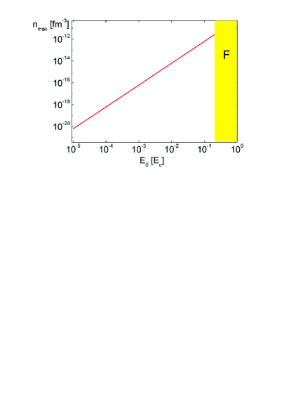
Figure 2: The dependence of $n_{\rm max}$ on the field strength $E_{0}$ in the calm valley.

In the following subsections we discuss the three characteristic domains of Fig. 1 separately.

III.1 The calm valley domain

This domain corresponds to the most simple behaviour of the distribution function characterized by the absence of an appreciable production rate for EPP when averaged over the period of field oscillation.

It is interesting to consider the initial behaviour of the distribution function $f(\textbf{p})$ immediately after the field is switched on. In Fig. 3 we present the typical form of $f(\textbf{p})$ at the time $t=T/4$, where $T=2\pi/\nu$ is the period of the laser field oscillation.

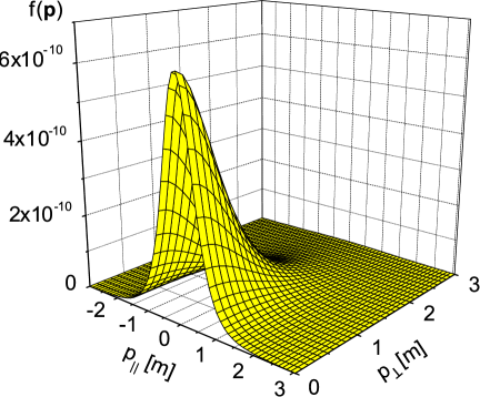
Figure 3: The EPP distribution function $f(p_{\bot},p_{\parallel})$ for the laser radiation with $\lambda=1$ nm and $E=10^{-4}E_{c}$ at the moment $t=T/4$.

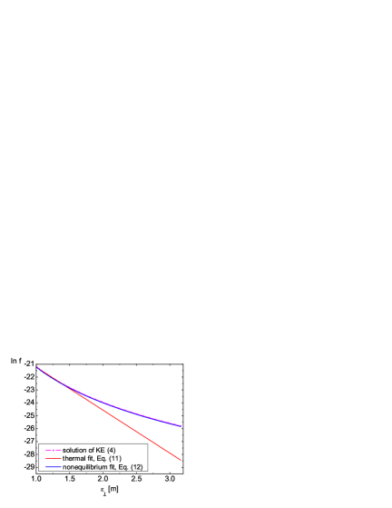
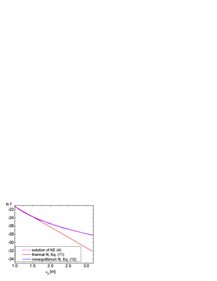
Figure 4: Fitting the KE solution $f(\textbf{p},t=T/4)$ of Fig. 3 (dash-dotted line) with an anisotropic equilibrium Boltzmann distribution (11) with $T_{\perp}=0.3~{}m$ (upper panel) and $T_{\parallel}=0.19~{}m$ (lower panel) as well as with a power-like distribution (12).

This distribution is anisotropic and can be approximated by a two-temperature Boltzmann distribution

$$f_{\rm eq}(p_{\perp},p_{\parallel})\sim\exp{\{-\varepsilon_{\perp}/T_{\perp}-\varepsilon_{\parallel}/T_{\parallel}\}}~{},$$ (11)

where $T_{\perp}$ is the transversal and $T_{\parallel}$ the longitudinal temperature while $\varepsilon_{\parallel}(\textbf{p})=\sqrt{m^{2}+p_{\parallel}^{2}}$ is the longitudinal energy. Fig. 4 demonstrates the similarity of the distributions $f(\mathbf{p})$ and $f_{eq}(\mathbf{p})$ (11) and the relation for the temperatures $\xi=T_{\parallel}/T_{\perp}$. However, a more satisfactory approximation for the pair distribution function is

$$f_{\rm in}(\textbf{p})\sim\varepsilon^{2}_{\perp}(p_{\perp})/\omega^{6}_{0}(\textbf{p})~{}.$$ (12)

The difference between the distributions (11) and (12) appears in the high-energy tails. The estimate (12) can be obtained on the basis of the KE (4) in the low density approximation in the multiphoton domain $\gamma\gg 1$ (see also Sect. IV). In the framework of the approximation (11) the temperature parameters $T_{\perp}$ and $T_{\parallel}$ are universal and do not depend on the laser field parameters $\lambda$ and $E_{0}$. In these assumptions the distributions (11) and (12) are independent of the wavelength $\lambda$ and proportional to $E_{0}^{2}$. Moreover, in the initial stage these estimates remain valid regardless of the form of the electric field pulse. This holds in particular for the Sauter potential, where the solution is well known Nikishov:1969tt ; Narozhnyi:1970uv ; Grib:1994 .

The excitation mechanism of the anisotropic spectrum of EPPs in the early stage of the evolution is fully determined by the dynamics of vacuum creation and, specifically, by the structure of the amplitude (5). There the anisotropy effects are represented by both, the transverse energy $\varepsilon_{\perp}(p_{\perp})$ and the quasienergy $\omega(\mathbf{p},t)$. The same anisotropy factor $\xi=2/3$ can be obtained on the basis of the distribution (12), when the relation of derivatives of the projections $f_{in}(p_{\parallel},p_{\perp}=0)$ and $f_{in}(p_{\parallel}=0,p_{\perp})$ with respect to $\varepsilon_{\parallel}$ and $\varepsilon_{\perp}$ is considered.

Thus, in the case of a short pulse, the anisotropic distributions (11) and (12) will lead to an elliptic flow of EPPs, which is compressed in the direction of the electric field.

The estimates (11) and (12) are modified when other mechanisms of vacuum creation of fermions are realized (see, e.g., Filatov:2007ha ). This can lead to a change of the anisotropy factor $\xi$. Considering, instead of fermions, the case of bosons, the situation changes radically: the equilibrium-like distributions of the type (11) and (12) are replaced by the ones for strong nonequilibrium Schmidt:1998zh , see Fig. 5.

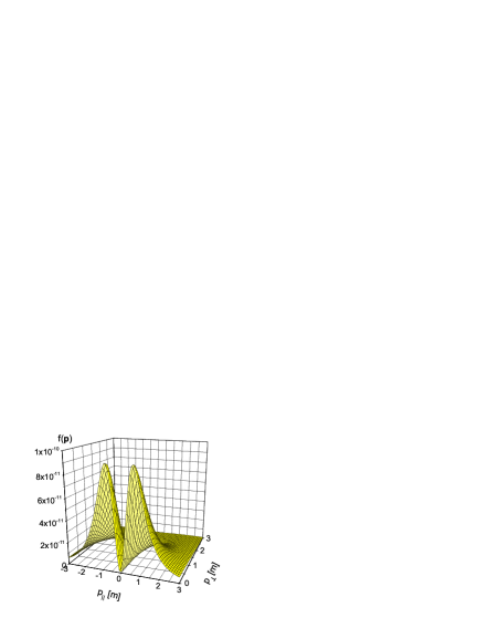
Figure 5: Momentum space distribution of bosons for the same conditions as in Fig. 3.

Thus, one can say that the initial distribution of the particles created from vacuum is well defined in the general case. In particular, the conclusion about the existence of equilibrium-like universal distributions can become important for the theory of quark-gluon plasma generation in heavy-ion collisions.

A few remarks are in order. Apparently, the temperature parameters $T_{\perp}$ and $T_{\parallel}$ can not be interpreted as the Unruh temperature $T_{U}=a/2\pi$ Castorina:2007eb , since the acceleration $a=-(e/m)\dot{A}(t)\sim E_{0}$ would imply a field dependence of $T_{\perp}$ and $T_{\parallel}$ which is not observed in our numerical investigations. Some anisotropic initial distributions of particles created from vacuum under the action of an electric field have been introduced long ago (see, e.g., Ruffini:2009hg ), but they have artificial character.

While a parametrization of the distribution function resulting from the KE (4) by a Boltzmann distribution may be a covenient characterization at certain time instances and in restricted intervals of momenta or energies, the concept of temperature in the usual thermodynamical or statistical sense is obviously not applicable. In the present example, it is the strong anisotropy which signals a striking off-equilibrium situation not accessible by equilibrium or near-equilibrium thermodynamics.

Such a simplifying picture of the phenomena in the calm valley is valid approximately in the initial stage of the process for $t\lesssim T$. The high frequency harmonics become essential at $t\gg T$ and the structure of the distribution function gets very complex. However, the amplitude estimate remains valid and the EPP production rate averaged over a period (i.e., the pair creation per unit time) is absent, $<\dot{f}>_{T}\approx 0$. The dependence $n_{\rm max}(E_{0})$ as depicted in Fig. 2 reveals that in the whole calm valley domain holds $n_{\rm max}(E_{0})\sim E^{2}_{0}$ up to the strong field accumulation region (the shaded area “F” in that figure) where the numerical calculation is complicated. The distribution function $f(\textbf{p},t)$ shows a breathing oscillation with the amplitude $f_{\rm max}$ and a frequency being twice that of the laser field (see Fig. 6, dashed line).

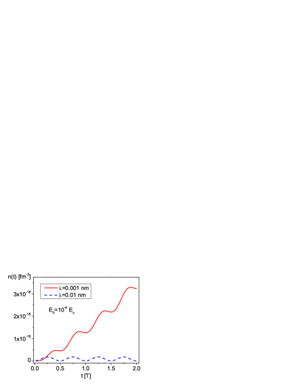
Figure 6: Time dependence of density $n(t)$ in the weak field regime evidencing the transition from the oscillating mode for $\lambda=0.01$ nm to the linearly growing (in the mean) mode at $\lambda=0.001$ nm. The latter behaviour is termed here as “accumulation”.

These features of the distribution function behavior are reproduced very well analytically on the quasiparticle level in Sect. IV. The residual number density of EPP is very small in comparison with the breathing mode.

The calm valley is bounded from above and to the left by the two accumulation domains F and R (see Fig. 1), where the amplitude of the distribution function increases with the lapse of time and the averaged EPP production rate $<\dot{f}>_{T}$ becomes appreciable. Apparently, a glimpse of accumulation effect is presented in the calm valley too. However, this effect is negligibly small for $\nu\ll m$ and $E_{0}\ll E_{c}$. Thus, the accumulation effect becomes dominant in the F and R domains only.

III.2 The resonance accumulation domain

This domain starts in the short wavelength domain from the point $\lambda_{\rm acc}\approx\pi\hskip 2.84526pt\vspace{2mm}\bar{}\vspace{-2mm}\lambda_{C}=0.0012$ nm, corresponding to the energy $\nu=2m$, which peaks out from the monochromatic external field for creation of an EPP. We will denote this process as one-photon pair creation. Below we will use this term in the analysis of solutions of the KE (4), for which the spatial inhomogeneity effects are negligible. Here, in the point $\lambda_{\rm acc}$ the accumulation mechanism is switched on sharply. As an example, the initial growth of the density in the course of time is depicted in Fig. 6 for $\lambda=0.001$ nm and $E_{0}=10^{-4}~{}E_{c}$. At the later stages the degeneration effect developes. Here the distribution function reaches its maximal value and after that it performs oscillations which are damped asymptotically (see Fig. 7). In addition, the $2\nu$-dependence of the breathing mode is conserved in the R domain.

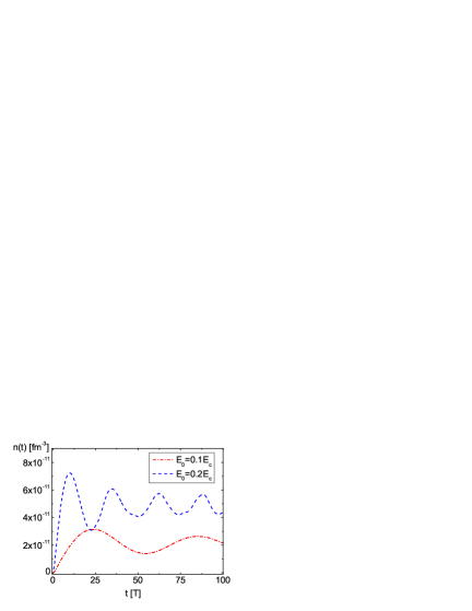
Figure 7: The limitation of accumulation due to the saturation of $f(\textbf{p})$ at large times for $\lambda=0.001$ nm. The saturation is achieved faster for stronger fields.

The shape of the distribution function is changes rapidly. Later on, for $\lambda\leq\lambda_{\rm acc}$, it leads to a collapse of the distribution function in a thin spherical layer (EPP bubble, see Figs. 8 and 9).

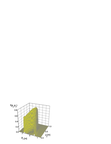
Figure 8: The distribution function $f(p_{\bot},p_{\parallel})$ in the R domain at time $t\gg T$. Most of pairs are seen within a thin spherical layer centered at the origin of the coordinates.

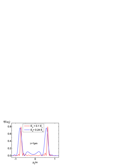
Figure 9: The $f(0,p_{\parallel})$ dependence in the R domain at large times after saturation for different field strengths.

The thickness $\Delta p$ and the size of this layer depend on the field parameters $\lambda$ and $E_{0}$. For example, for $\lambda=0.001$ nm and $E_{0}=0.24~{}E_{c}$ we have $\Delta p\sim 0.1~{}m$. With growing field strength at a fixed frequency the maximum value $f_{\rm max}(\textbf{p})$ increases in the degeneration condition, $f_{\rm max}(\textbf{p})\to 1$. The occupation of the EPP bubble increases also (Fig. 9) under this condition (appearance of some thin wave structure arises within the bubble). On the other hand, the decrease of the wavelength in the domain $\lambda\lesssim\lambda_{acc}$ does not change the distribution picture essentially (see Fig. 10).

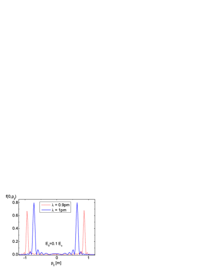
Figure 10: The $f(0,p_{\parallel})$ dependence in the R domain at large times after saturation for different wavelengths.

The radius of the EPP bubble in momentum space is equal to

$$p_{\rm bub}=\sqrt{(\pi/\lambda)^{2}-m^{2}}~{}~{}{\rm for}~{}~{}\lambda\leq\lambda_{\rm acc}~{}.$$ (13)

For $\nu\to 2m$, this radius goes to zero, $p_{\rm bub}\to 0$ (it corresponds to the condition $\nu=2m$ or the point $\lambda=\lambda_{acc}$). Decreasing the wavelength is accomplished by the growth of the EPP bubble size (see Fig. 10). The maximal value of the number density of the vacuum bubble in the saturation state (see Fig. 11) and the time period necessary for achieving the saturation (see Fig. 12) show that the first passage time of the saturation grows indefinitely with decreasing $\lambda<\lambda_{acc}$.

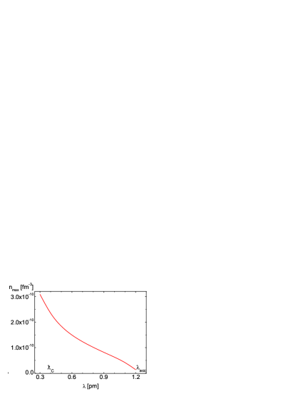
Figure 11: The dependence of $n_{max}$ on wavelength $\lambda$ in the R domain for $E_{0}=0.1~{}E_{c}$.

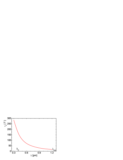
Figure 12: The dependence of the saturation time $\tau_{s}$ on the wavelength $\lambda$ in the R domain for $E_{0}=0.1~{}E_{c}$

From Fig. 1 it follows that the point $\lambda_{\rm acc}$ lies on the left of the critical line $\gamma=1$ in the domain $\gamma\gg 1$, where the multiphoton mechanism of EPP excitation is operative. Apparently, one can expect that the multi-photon process can be changed to a few-photon one in the lower left part of this figure. As the result, the few-photon domain is limited by the two- and one-photon processes. For weak fields $E\ll E_{c}$, the one-photon process of the EPP creation dominates (this conclusion is confirmed by the analytical calculations in Sect. IV). The two-photon pair creation process (the inverse of the Breit-Wheeler process Berestetskii ; Ruffini:2009hg ; 854971 ) is switched on for rather strong field $E_{0}\sim E_{c}$ beginning with $\lambda_{2\gamma}=\lambda_{C}=2\lambda_{\rm acc}$, see Fig. 13.

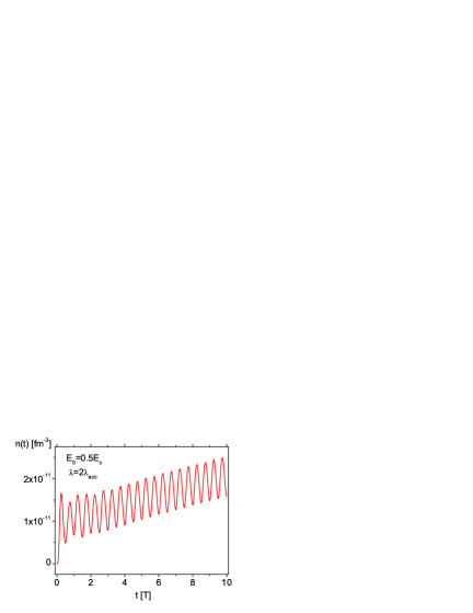
Figure 13: Transient region from calm valley to F accumulation: the characteristic for F domain with linear growth of mean density is here caused by the subcritical field $E_{0}=0.5E_{c}$, at the wavelength for the opening of the two-photon production channel $\lambda=\lambda_{C}=2\lambda_{\rm acc}$.

This domain is characterized by the fast growth of the EPP density and it is contained in the F accumulation domain. Surprisingly, the KE (4) is sensitive to this effect which is valid in the case of a quantized electromagnetic field. Let us remark that the one-photon mechanism of EPP excitation prolongs to act in all domains of short wavelengths $\lambda<\lambda_{\rm acc}$.

After having discussed implications of the purely periodic field (3) we turn now to two other examples of the time dependence. The initial condition is $f(t\to-\infty)=0$.

For the first time, some features in the behaviour of the EPP distribution function in the domain of extremely short wavelengths ($\lambda\sim\lambda_{C}$) were observed theoretically for the residual EPP at $t\to\infty$ in the framework of different approaches taking into account a spatial inhomogeneity of the external electric field in the works Hebenstreit:2011wk ; Gies:2005bz ; Dunne:2006ur . In the present work we investigate the behavior of the quasiparticle EPP within a period of the laser pulse action. It is well known that the properties of the real (residual) and quasiparticle EPP differ strongly (see, e.g., Fig. 14). It is possible that just this feature explains the difference between the results of the present work and Refs.  Hebenstreit:2011wk ; Gies:2005bz ; Dunne:2006ur regarding the short distance behaviour of the EPP. In the framework of the formalism based on the KE (4) such a comparison shall be performed within a separate work subsequent to this. On the other hand, as pointed out above, the Q domain (Fig. 1) is the domain of unreliable predictions obtained on the basis of an extrapolation of the domain of applicability of the KE (4) limited by the quasiclassical external electric fields where the electromagnetic fluctuations are inessential.

III.2.1 Gaussian envelope

Let us investigate first the PV response to the action of a pulsed field with Gaussian temporal envelope

$$E(t)=E_{0}\sin{(\nu t)}\exp{(-t^{2}/\tau_{G}^{2})}~{}.$$ (14)

The comparison of the accumulation effects for the periodical field (3) with $\lambda=0.001$ nm (dashed line) and the corresponding field pulse (14) with $\tau_{G}=10$ T is shown in Fig. 14. It allows to draw the conclusion that the form of the field pulse is rather essential but it does not change qualitatively the picture of the effect. The switching-off process of the pulse (14) is accompanied by a stepwise reduction of the EPP density down to some residual level, see Fig. 14, which should be compared with Fig. 6. Let us remark that in the regime of saturation the residual EPP density can surpass considerably the amplitude of the breathing oscillations while in the calm valley the situation is opposite.

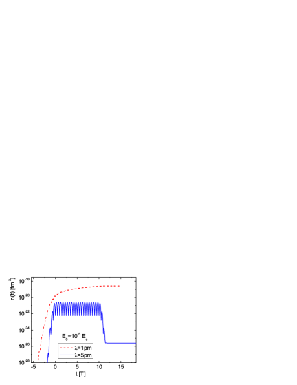
Figure 14: Transition from the oscillating mode (for $\lambda=5$ pm) to the accumulation mode (for $\lambda=1$ pm) for the pulse (14) with $\tau_{G}=10$.

III.2.2 Sauter pulse

Now we consider action of a smooth pulse field with the Sauter potential

$$A(t) = -E_{0}\tau_{S}\tanh{(t/\tau_{S})}~{},$$ (15)

$$E(t) = E_{0}/\cosh^{2}{(t/\tau_{S})}~{}.$$ (16)

Similar to the field (14) one can clearly define here the residual density $n_{\rm out}=n(t\to\infty)$. The typical resonance picture is revealed here with the maximum at $\tau_{S}\approx 1/2m$, see Figs. 15 and 16.

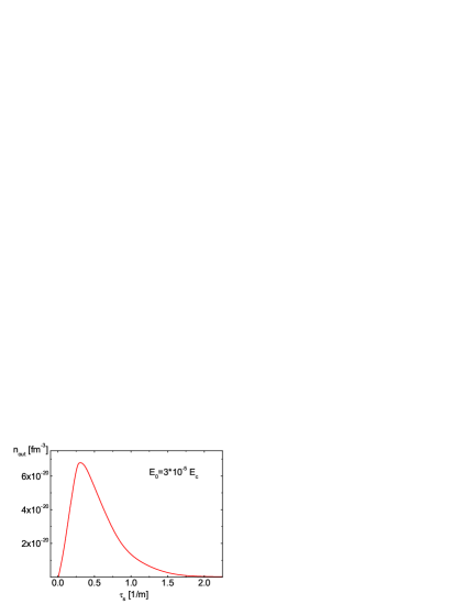
Figure 15: The residual pair density $n_{\rm out}$ as a function of $\tau_{S}$ for the pulsed field (16).

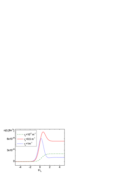
Figure 16: The time dependence of pair number density for the pulsed field (16) for three values of the pulse length parameter $\tau_{S}$.

For $\tau_{S}\ll 1/2m$ a sharp decrease of the PV response takes place and the vacuum EPP creation practically ceases. This result corresponds to the conclusion of Ref. Hebenstreit:2011wk . The characteristic value $\tau_{S}=1/2m$ allows to speak here about the influence of one-photon pair production process on the level of the kinetic description. This feature in the solution of the KE (4) with the potential (15) can be confirmed also by an analysis of the exact solution of the problem Narozhnyi:1970uv .

The accumulation effect in the R domain can be explained if one takes into account the presence in the solution of the KE (4) of a parametric resonance in the neighborhood $\nu=2m$ and of all combinational frequencies $n\nu$ and $2ml$, where $n$ and $l$ are the integers and the factor 2 is stipulated by the structure of the high frequency phase (6). This is compatible with a parity odd distribution function $f(\mathbf{p},t)$ under time reversal. It leads to the appearance of contributions of the type

$$\frac{1}{\nu-2m}\ \sin{(\nu-2m)t}\,\cdot\,\sin{(\nu+2m)t}~{}.$$ (17)

For $\nu\sim 2m$ a secular term appears here that results in a linear growth of the distribution function. The subsequent evolution is accompanied by a growth of the EPP number density and saturation as a result of the action of the statistical factor in the KE (4). Just this picture is observed for the numerical solution in the R-accumulation domain. The given interpretation was generated by the perturbation theory in the low density approximation, see Sect. IV.

Let us remark also that the motion along the $\lambda$-axis on the side of short waves is accompanied by a sequential replacement of the vacuum creation mechanisms: the tunneling mechanism acts in the limit of stationarity ($\lambda\to\infty$) and slowly alternating field and requires an infinite photon number from the external field reservoir. This mechanism is then replaced by the multiphoton ($\gamma\gg 1$) and few-photon ones and finally turns into the one- and two-photon pair production. It is necessary to underline that the conception of the ”photon” is considered here in the framework of the accepted model of the spatially homogeneous electric field acting in the focal spot of counter propagating laser fields with the linear size $\sim\lambda$ that allows to use in the description of the absorption processes the energetic condition only (e.g., $\nu=2m$ for the one-photon $e^{-}e^{+}$ production process).

III.3 The strong field accumulation domain

After the interlude on finite pulses let us return to the discussion of further effects related to the periodic field (3). For the first time, the accumulation effect in a strong laser field (domain F in Fig. 1) was discovered in Ref. Alkofer:2001ik and further explored in Roberts:2002py on the basis of a numerical solution of the KE (4). The accumulation domain begins here with a rather high field strength $E_{0}\approx 0.2E_{c}$. The smooth breathing mode with a smooth phase space distribution (Fig. 3) is replaced here by a strongly fragmented one with pronounced structures (Fig. 17).

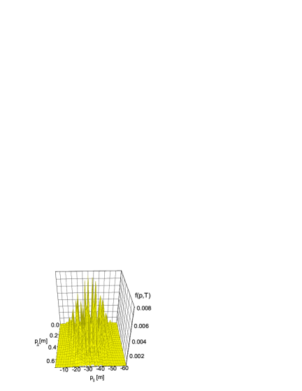
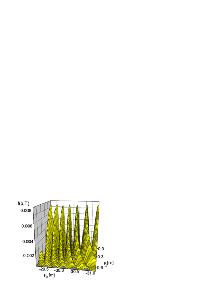
Figure 17: The distribution function in the F accumulation domain at $t=T$ ($E_{0}=0.5~{}E_{c},~{}\lambda=0.15$ nm). Upper panel: general view; lower panel: detailed view highlighting the concentric dense layers.

Apparently, in the long wavelength limit the usual accumulation mechanism acts here. For the transition to the observable domain, the electron and positron must gather within a spatial extent of one Compton wavelength, an energy which is comparable to the energy gap, i.e. $eE_{c}\hskip 2.84526pt\vspace{2mm}\bar{}\vspace{-2mm}\lambda_{C}=2m$. In the multi- and few-photon domains the other mechanism is switched on where the EPP creation is a result of the simultaneous absorption of $n$ identical photons from the ”photon reservoir” of the laser field. The probability for such kind of process, in principle, can be taken into account on the basis of an analogy with the theory of multiphoton ionization of atoms given, e.g., in Ref. Delone:1998 .

The intersection region of the two accumulation domains R and F (the left top corner on Fig. 1) is especially interesting. Here the nonlinear superposition of two accumulation effects can lead to some new features in the vacuum EPP production which have been investigated in recent years under the name of “dynamically assisted Schwinger mechanism” Schutzhold:2008pz ; Orthaber:2011cm ; Fey:2011if . It is important that the applicability of the KE (4) is not violated in this domain.

Thus, the accumulation processes in the R and F domains are the processes of the EPP excitation up to the saturation state and next increasing of EPP density in this state. Let us note that the vacuum response reveals the symmetry of the states in a weak ($E_{0}\ll E_{c}$) and a strong ($E_{0}\sim E_{c}$) field, respectively: under the substitution $f=1-\tilde{f}$ in the KE (4) it does not change its form and the case $f\ll 1$ is similar to the case $\tilde{f}\ll 1$.

IV Low density approximation

The numerical results discussed in Sect. III can be confirmed analytically in the multiphoton domain ($\gamma\gg 1$) of the calm valley. From the KE (4) it follows in the low density approximation $f\ll 1$ corresponding to $E_{0}\ll E_{c}$ Blaschke:2010sgu that

$$f(\mathbf{p},t)=\frac{1}{4}\bigg{|}\int^{t}_{t_{0}}dt^{\prime}\lambda(\mathbf{p},t^{\prime}){\rm e}^{2i\theta(t^{\prime},t_{0})}\bigg{|}^{2}.$$ (18)

This formula solves correctly the initial value problem in the KE (4) providing a vanishing distribution function both at $t\to t_{0}$ and $E_{0}\to 0$. In the leading approximation $\omega(\mathbf{p},t)\rightarrow\omega_{0}(\mathbf{p})=\sqrt{m^{2}+p^{2}}$ , corresponding to $\gamma\gg 1$, after the time integration, one arrives at

$$f(\mathbf{p},t)=f_{(0)}(\mathbf{p})+\frac{1}{2}f_{(2)}(\mathbf{p})[1-\cos 2\nu t],$$ (19)

where ($\alpha=e^{2}/4\pi$)

$$f_{(0)}(\mathbf{p}) = \pi\alpha E^{2}_{0}\frac{\nu^{2}\varepsilon^{2}_{\bot}}{\omega_{0}^{4}[4\omega_{0}^{2}-\nu^{2}]^{2}},$$ (20)

$$f_{(2)}(\mathbf{p}) = {\pi\alpha E^{2}_{0}}\frac{\varepsilon^{2}_{\bot}}{\omega_{0}^{4}|4\omega_{0}^{2}-\nu^{2}|}.$$ (21)

In these calculations, the assumption of adiabatically switching-on the electric fields (1) at $t_{0}\rightarrow-\infty$ was made.

The leading role of the second harmonics (19) was detected in the numerical solutions of the KE (4) (see Sect. III) and used in Blaschke:2008wf ; Blaschke:2005hs with the amplitudes $f_{(0)}$ and $f_{(2)}$ as the results of the numerical analysis.

The $E_{0}^{2}$ dependence of $f_{\rm max}$ and $n_{\rm max}$ (see Fig. 2) follows immediately from Eqs. (20) and (21). The time dependent component (21) does not depend on $\nu$ for $\nu\ll m$ (see Fig. 1, calm valley); the constant component (20) brings some small dependence in this domain. The calculations close to the poles in Eqs. (20) and (21) require a more careful analysis. The Eqs. (20) and (21) indicate the one-photon mechanism of the EPP bubble generation in the resonance domain $\nu\simeq 2\omega_{0}(\mathbf{p})$ (see Sect. III, Subsect. III.2). In the considered approximation this bubble has a spherical form.

The estimates of the density (10) on the basis of Eqs. (20) and (21) lead to the result

$$n(t)=n_{(0)}+\frac{1}{2}n_{(2)}[1-\cos(2\nu t)]~{}.$$ (22)

In the leading approximation with respect to small $\nu/\omega_{0}$ it follows from Eqs. (20) and (21) that

$$n_{(0)} = \frac{5}{3}\frac{\alpha}{m}\left(\frac{E_{0}}{16}\right)^{2}\biggl{(}\frac{\nu}{m}\biggr{)}^{2}~{},$$ (23)

$$n_{(2)} = \frac{3}{2}\frac{\alpha}{m}\left(\frac{E_{0}}{4}\right)^{2}~{}.$$ (24)

The ratio of these expressions is equal to $n_{(0)}/n_{(2)}=(5/72)(\nu/m)^{2}$ , which is close to the estimate given in Blaschke:2005hs . The frequency independence and $E_{0}^{2}$ dependence of the amplitude $n_{(2)}$ of the number density oscillations agrees with the numerical calculations exhibited in Fig. 1. The constant (residual) component density (23) was not observed previously in numerical calculations. The numerical integration shows that the estimates (23) and (24) remain valid up to the quasiclassical boundary $\nu\lesssim 2m$. The asymptotics at $\nu\to 0$ in Eqs. (20) and (23) leads to a vanishingly small residual EPP density.

Thus, in the multiphoton domain of the calm valley the averaged production rate $<\dot{f}>_{T}$ of EPP is negligibly small. Instead, there are vacuum oscillations induced by the external field and the small constant (residual) component. In principle, these vacuum effects can lead to some observable effects. For instance, they influence on the propagation of an electromagnetic probe signal. This can result in an anomalous absorption of this signal at the frequency $2\nu$.

The perturbation theory used here in the quasiparticle representation is valid in the multiphoton domain $\gamma\gg 1$, when the swing amplitude (Sect. III) is small. However, the numerical solutions of the KE (4) show that these results are valid also in some parts of the tunneling mechanism region. At first glance, this fact is unexpected. Indeed, in this region for subcritical fields $E_{0}\ll E_{c}$ it is very well known that the EPP production rate is exponentially small Grib:1994 ; Brezin:1970xf . But this effect is not accessible to perturbation theory. On the other hand, the domain of the long wavelength limit $\lambda\gtrsim\lambda_{0}$ is difficult for the numerical analysis and it was not studied in the present work. It is possible, that some special solution of KE (4) is present here which is compatible with the well known estimates Grib:1994 ; Brezin:1970xf .

V Summary

In the present work we have described the PV response to a monochromatic laser radiation in the landscape of the laser parameters (1) and (2). Three specific domains were observed here

• the domain of the vacuum oscillations induced by the external field (calm valley), where the EPP production rate is very small, $<\dot{f}>_{T}\approx 0$, and the breathing modes are acting only,

• the domain of the accumulation effect due to strong field (F), and

• the resonant (R) accumulation domain, where the EPP production rate can reach significant values.

Thus, it was shown that the behavior of the PV in the calm valley up to a certain critical point $\lambda_{acc}=\pi\hskip 2.84526pt\vspace{2mm}\bar{}\vspace{-2mm}\lambda_{C}$ is stable and does not depend on the wavelength $\lambda$ of the external electromagnetic field. This domain accommodates different mechanisms of vacuum decay into quasiparticle EPP excitations

• tunneling ($\gamma\ll 1$, when the photon number of the external field is infinity or very large),

• multiphoton processes ($\gamma\geq 1$) and

• few-photon processes.

The accumulation effect depicted in Fig. 1, appears just either in the multiphoton domain as a parametric resonance induced by the one-photon mechanism of EPP creation at the frequency $\nu=2m$ (domain R) or as a result of the acceleration of quasiparticle $e^{-}e^{+}$ pairs in a subcritical external field (domain F). These processes are accompanied by the accumulation of EPP density and are limited by the condition $f(\mathbf{p},t)\leq 1$. For increasing $E_{0}$, the domain of the momentum space covered by the distribution function is enlarged too (”broadening” of $f(\mathbf{p},t)$, see Fig. 7). This can lead to a rapid growth of the EPP density.

For the strong and moderately strong fields (see Fig. 1) these predictions are based on a realistic KE (4) in the scope of its applicability. For sufficiently small fields, $E_{0}\ll E_{c}$, the accumulation R-domain comes in the region of the strongly fluctuating external fields, where the KE (4) is not applicable, generally speaking, and its solutions have here only exploratory character.

As the EPP density under the accumulation conditions in the R domain can be very high even for relatively weak fields, $E_{0}\ll E_{c}$, it can be expected that the manifestation of the dynamical Schwinger effect can be quite possible in this domain due to the generation of secondary effects such as, e.g., the radiation of annihilation photons. Apparently, these remarks can be useful for the discussion of possible experiments for observing the dynamical Schwinger effect. On the other hand, the accumulation effect in the both accumulation domains R and F in the short-wavelength domain can be considerable only for a sufficiently long duration of the laser field action $t\gg T$ (Figs. 6, 7 and 14). This circumstance makes difficult an experimental observation of the effect in the case of a short single laser pulse.

In the theory of vacuum EPP creation under the action of a periodic laser field of the type (3) the residual EPP density is the basic final product of the theory. However, its definition can be difficult. In the present work the residual density is understood, as a rule, as the EPP density at the final moment of action of some field periods (see, e.g., Grib:1994 ; Brezin:1970xf ). It corresponds to the density $n_{(0)}$ (23). In such a case it is implied that the field (3) either prolongs to act farther than the periodical field or it switches off instantly. Both these cases are rather artificial. It would be more satisfactory to consider some pulsed field of the type (14), when a periodical field switches on and off gradually or adiabatically. The similar situation was discussed in the Sect. III. It is very important that it does not lead to qualitative change in the picture for moderate fields thus demonstrating the stability of the obtained results with respect to the way of switching the laser field on and off.

Let us underline also that the approach used in the present work is based on a minimal number of very general assumptions (spatial homogeneity of the external field and its linear polarisation) and is in essence an exact consequence of the basic QED in the framework of these limitations. This circumstance allows the authors to express the opinion that the obtained results in the framework of the given approach are free from some additional approximation (e.g., of the WKB type) and therefore a more trustworthy in the QC-domain. Moreover, they allow to make first prognoses for the Q-domain. On the other hand, the basic kinetic equation (KE) (4) is valid in the case of a quasiclassical electric field (3) only. We extrapolated the domain of its applicability into the Q domain. The foundation for such an extrapolation is the assumption that the solution of the KE (4) in the boundary domain is valid approximately because there the quantum fluctuations of the electric field are not too large. Thus, we observe here the tendency to a non-monotonicity described above. In the Q domain the external field can be described with the help of the corresponding density matrix of the electromagnetic field. Then, the quasiclassical field $A^{\mu}$ will play the role of a background field, i.e. $A_{tot}^{\mu}=A^{\mu}+\hat{A}^{\mu}$, where $\hat{A}^{\mu}$ is the field operator of the photon component of the total field $A_{tot}^{\mu}$.

For a more adequate investigation of the PV response in the Q domain it is necessary to develop a kinetic theory for the generalization of the KE (4) taking into account the quantum fluctuations of the electric field. For understanding the situation, we mention the works Krive:1984xi ; Popov:2002 in which the vacuum particle creation is considered under the influence of a stochastic time dependent electric field. We want to mention two of the possibilities which emerge here. The compressed state of the electromagnetic field (e.g., Bykov:1991 ) is a quantum one but contains a large occupation number of photons. As a result, the criterion (6) of the quasiclassical case can be not adequate to this situation. For the second example we remark that, in the case of a rather strong field $E_{0}\gtrsim 0.1~{}E_{c}$, the backreaction mechanism becomes essential and leads to a stochastic (or close to one) internal electric field Vinnik:2001qd . Thus, the kinetic description of vacuum particle creation in the Q domain is an actual problem deserving further investigation.

Considering the muon PV independently of $e^{-}e^{+}$ PV, it can be expected that the response of the $\mu^{-}\mu^{+}$ PV will repeat on the qualitative level the picture described in Sect. III with a shift to the side of shorter waves.

Two regions in the plane of the parameters (1) and (2) remain uninvestigated in the framework of the used approach: the top left corner on Fig. 1 where short wavelengths and strong fields simultaneously persist, and the right boundary of the tunneling domain in the calm valley where $\lambda>\lambda_{0}$. It would be worthwhile to investigte these areas separately. Preliminary results of this work have been reported recently Dresden2011 and a more elaborate discussion is in preparation.

VI Conclusion

We have investigated the behavior of the quasiparticle EPP generated from the PV under the action of a strong laser field. It was shown that particle production in the initial stage of the field action is characterized by an equilibrium like “thermal” distribution. However, at later times the quasiparticle EPP distribution becomes very complicated and shows a far-from-equilibrium behaviour with distinct features depending on the specific domain of the landscape. In the subsequent, second part of the work we plan to investigate features of the real EPP which remains after the laser pulse ceases. Moreover, the transient phenomenona between quasiparticle and residual states of the EPP shall be studied.

Acknowledgements

We are grateful to A. M. Fedotov, L. Juchnowski, A. G. Lavkin, A. V. Tarakanov and V. D. Toneev for useful discussions on different aspects of this work. The work of D.B.B. was supported in part by the Russian Fund for Basic Research under grant No. 11-02-01538-a. S.A.S. and S.M.S. acknowledge support by Deutsche Forschungsgemeinschaft (DFG) under Project number TO 169/16-1.

References

- (1) G. Baur, Nucl. Phys. Proc. Suppl. 184, 143 (2008).
- (2) V. V. Dodonov, Phys. Scripta 82, 038105 (2010).
- (3) Y. Kluger, J. M. Eisenberg, B. Svetitsky, F. Cooper and E. Mottola, Phys. Rev. D 45, 4659 (1992).
- (4) S. M. Schmidt, D. Blaschke, G. Röpke, S. A. Smolyansky, A. V. Prozorkevich and V. D. Toneev, Int. J. Mod. Phys. E 7, 709 (1998).
- (5) V. N. Pervushin and V. V. Skokov, Acta Phys. Polon. B37, 2587 (2006).
- (6) D. B. Blaschke, A. V. Prozorkevich, C. D. Roberts, S. M. Schmidt and S. A. Smolyansky, Phys. Rev. Lett. 96, 140402 (2006).
- (7) D. B. Blaschke, S. M. Schmidt, S. A. Smolyansky and A. V. Tarakanov, Phys. Part. Nucl. 41, 1004 (2010).
- (8) D. B. Blaschke, G. Röpke, S. M. Schmidt, S. A. Smolyansky and A. V. Tarakanov, Contrib. Plasma Phys. 51, 451 (2011).
- (9) S. A. Smolyansky, D. B. Blaschke, A. V. Chertilin, G. Röpke and A. V. Tarakanov, [arXiv:1012.0559 [physics.plasm-ph]].
- (10) D. B. Blaschke, G. Röpke, V. V. Dmitriev, S. A. Smolyansky and A. V. Tarakanov, arXiv:1101.6021 [physics.plasm-ph].
- (11) D. B. Blaschke, V. V. Dmitriev, G. Röpke and S. A. Smolyansky, Phys. Rev. D 84, 085028 (2011).
- (12) A. Di Piazza, K. Z. Hatsagortsyan and C. H. Keitel, Phys. Rev. Lett. 97, 083603 (2006).
- (13) F. Sauter, Z. Phys. 69, 742 (1931).
- (14) W. Heisenberg and H. Euler, Z. Phys. 98, 714 (1936).
- (15) J. S. Schwinger, Phys. Rev. 82, 664 (1951).
- (16) W. Greiner, B. Müller and J. Rafelski, ”Quantum Electrodynamics Of Strong Fields,” Berlin, Germany: Springer (1985).
- (17) A. A. Grib, S. G. Mamaev and V. M. Mostepanenko, Vacuum Quantum Effects in Strong External Fields, Friedman Laboratory Publish., St. Petersburg (1994).
- (18) E. Brezin and C. Itzykson, Phys. Rev. D 2, 1191 (1970).
- (19) N. B. Narozhny, S. S. Bulanov, V. D. Mur and V. S. Popov, Phys. Lett. A 330, 1 (2004); JETP Lett. 80, 382 (2004) [Pis’ma Zh. Eksp. Teor. Fiz. 80, 434 (2004)].
- (20) N. B. Narozhny, S. S. Bulanov, V. D. Mur and V. S. Popov, Zh. Eksp. Teor. Fiz. 129, 14 (2006) [JETP 102, 9 (2006)].
- (21) A. M. Fedotov, Laser Phys. 19, 214 (2009).
- (22) D. B. Blaschke, A. V. Prozorkevich, G. Röpke, C. D. Roberts, S. M. Schmidt, D. S. Shkirmanov and S. A. Smolyansky, Eur. Phys. J. D 55, 341 (2009).
- (23) A. V. Filatov, A. V. Prozorkevich and S. A. Smolyansky, Proc. of SPIE 6165, 616509 (2006).
- (24) A. V. Filatov, S. A. Smolyansky and A. V. Tarakanov, Proc. of the XX International Baldin Seminar on High Energy Physics Problems ”Relativistic Nuclear Physics and Quantum Chromodynamics”, Dubna, Sept. 29 - Oct. 04, 2008, 202 (2008).
- (25) V. B. Berestetskii, E. M. Lifshits and L. P. Pitaevskii, Quantum Electrodynamics, Pergamon, New York (1982).
- (26) V.I. Ritus, Tr. Fiz. Inst. Akad. Nauk SSSR 111, 5 (1979) (in Russian).
- (27) V. S. Popov, Sov. Phys. JETP 120, 315 (2001).
- (28) V. S. Popov, Phys. Usp. 47, 855 (2004).
- (29) N. B. Delone, V. P. Krainov, Phys. Usp. 41, 469 (1998).
- (30) D. B. Blaschke, V. V. Dmitriev, P. I. Smolyansky, S. A. Smolyansky and A. V. Chertilin, Proceedings of Saratov University, Ser. Physics, 10, 45 (2010) (in Russian).
- (31) B. Liesfeld, J. Bernhardt, K. U. Amthor, H. Schwoerer and R. Sauerbrey, Appl. Phys. Lett. 86, 161107 (2005).
- (32) G. Gregori, D. B. Blaschke, P. P. Rajeev, H. Chen, R. J. Clarke, T. Huffman, C. D. Murphy, A. V. Prozorkevich, C. D. Roberts, G. Röpke, S. M. Schmidt, S. A. Smolyansky, S. Wilks and R. Bingham, High Energy Dens. Phys. 6, 166 (2010).
- (33) A. Ringwald, Phys. Lett. B510, 107 (2001).
- (34) A. Di Piazza, C. Müller, K. Z. Hatsagortsyan and C. H. Keitel, Rev. Mod. Phys. 84, 1177 (2012).
- (35) A. V. Korzhimanov, A. A. Gonoskov, E. A. Khazanov and A. M. Sergeev, Phys. Usp. 54, 9 (2011).
- (36) R. Ruffini, G. Vereshchagin and S. -S. Xue, Phys. Rept. 487, 1 (2010).
- (37) S. M. Schmidt, D. Blaschke, G. Röpke, A. V. Prozorkevich, S. A. Smolyansky and V. D. Toneev, Phys. Rev. D 59, 094005 (1999).
- (38) G. Breit and J. A. Wheeler, Phys. Rev. 46, 1087 (1934).
- (39) F. Hebenstreit, R. Alkofer and H. Gies, Phys. Rev. Lett. 107, 180403 (2011).
- (40) H. Gies and K. Klingmüller, Phys. Rev. D 72, 065001 (2005).
- (41) G. V. Dunne and Q. -H. Wang, Phys. Rev. D 74, 065015 (2006).
- (42) A. I. Nikishov, Zh. Eksp. Teor. Fiz. 57, 1210 (1969) (in Russian).
- (43) N. B. Narozhnyi and A. I. Nikishov, Yad. Fiz. 11, 1072 (1970) [Sov. J. Nucl. Phys. 11, 596 (1970)].
- (44) A. V. Filatov, A. V. Prozorkevich, S. A. Smolyansky and V. D. Toneev, Phys. Part. Nucl. 39, 886 (2008).
- (45) P. Castorina, D. Kharzeev and H. Satz, Eur. Phys. J. C 52, 187 (2007).
- (46) R. Alkofer, M. B. Hecht, C. D. Roberts, S. M. Schmidt and D. V. Vinnik, Phys. Rev. Lett. 87, 193902 (2001).
- (47) C. D. Roberts, S. M. Schmidt and D. V. Vinnik, Phys. Rev. Lett. 89, 153901 (2002).
- (48) R. Schützhold, H. Gies and G. Dunne, Phys. Rev. Lett. 101, 130404 (2008).
- (49) M. Orthaber, F. Hebenstreit and R. Alkofer, Phys. Lett. B 698, 80 (2011).
- (50) C. Fey and R. Schützhold, Phys. Rev. D 85, 025004 (2012).
- (51) I. V. Krive and L. A. Pastur, Yad. Fiz. 39, 224 (1984) (in Russian).
- (52) A. M. Popov and O. V. Tikhonova, JETP 95, 844 (2002).
- (53) V. P. Bykov, Sov. Phys. Usp. 34, 910 (1991).
- (54) D. V. Vinnik, A. V. Prozorkevich, S. A. Smolyansky, V. D. Toneev, M. B. Hecht, C. D. Roberts and S. M. Schmidt, Eur. Phys. J. C 22, 341 (2001).
- (55) S. A. Smolyansky (in collaboration with D. B. Blaschke, A. M. Fedotov, A. G. Lavkin and A. V. Prozorkevich), Workshop ”Petawatt Lasers and Hard X-Ray Light Sources”, Dresden-Rossendorf, Sept. 5 to 9, 2011; http://www.hzdr.de/PWLasers2011.