Avalanches in the Raise and Peel model in the presence of a wall

Abstract

We investigate a non-equilibrium one-dimensional model known as the raise and peel model describing a growing surface which grows locally and has non-local desorption. For specific values of adsorption ($u_{a}$) and desorption ($u_{d}$) rates the model shows interesting features. At $u_{a}=u_{d}$, the model is described by a conformal field theory (with conformal charge $c=0$) and its stationary probability can be mapped to the ground state of the XXZ quantum chain. Moreover, for $u_{a}\geq u_{d}$, the model shows a phase in which the the avalanche distribution is scale invariant. In this work we study the surface dynamics by looking at avalanche distributions using Finite-size Scaling formalism and explore the effect of adding a wall to the model. The model shows the same universality for the cases with and without a wall for an odd number of tiles removed, but we find a new exponent in the presence of a wall for an even number of avalanches released. We provide new conjecture for the probability distribution of avalanches with a wall obtained by using exact diagonalization of small lattices and Monte-Carlo simulations.

I Introduction

The Raise and Peel Model (RPM) is a Markov process first proposed by gier describing the evolution of a growing surface with a fluctuating interface in one dimension. This model has been found to belong to a new universality class in non-equilibrium phenomena gier ; gier1 ; Alcaraz0 ; alcaraz ; alcaraz_facets . For a particular value of the adsorption ($u_{a}$) and desorption ($u_{d}$) rates, the model exhibits a phenomenon of self-organized criticality bak ; dhar where probability distributions of desorption events show long tails and are characterized by a varying critical exponent that depends on a single parameter given by the ratio of the adsorption and desorption rates alcaraz ; alcaraz_facets .

When adsorption and desorption rates are equal, the model becomes solvable. This goes back to a connection established by Razumov and Stroganov RS ; RStwisted ; gier2 which relates the two-dimensional dense $O(n=1)$ fully packed loop models (enumerating the stationary state probability distributions of RPM) to those a ground state wavefunctions of the XXZ chain with L sites alcaraz_facets ; Batchelor ; alcaraz_spin . Moreover, the spectra can be obtained by conformal field theory with charge c=0 Knops ; Henkel . This offers a nice mathematical structure, which allows to make conjectures using small lattices for expressions of physical quantities that remain valid for quantities for any system size.

In this work, we study the effect on avalanches in the presence of a wall (RPMW) since little is known about this effect when the boundary is allowed to fluctuate. Some other interesting results with the wall have been reported for example in Alcaraz2 ; Pyatov . In Section II we describe the stochastic rules for the model with and without a wall and highlight some of the known results for these two cases. In Section III, we compare the energy spectra of the stochastic Hamiltonian of the XXZ quantum chain for different spin sectors. Lastly in Section IV, we compute critical exponents for avalanche distributions for RPM and RPMW and derive new conjectures for probability expression with a wall.

II Raise and Peel Models

&

Figure 1: Three possible cases shown. (A) tile attaches to the surface, (B) tile removes a layer, (C) tile is reflected.

The Raise and Peel Model (RPM) describes a growing and fluctuating interface. An initial configuration is chosen and tiles are dropped onto the surface with a certain probability. Three different processes can happen as shown in figure II. With some probability $P_{i}=\frac{1}{L+a-1}$ a tile lands in site $i=1,...,L-1$, while in RPMW the site i=0 is chosen with some probability $P_{0}=\frac{a}{L+a-1}$. Depending on the slope of surface at the $i^{th}$ site, one of three things can occur.

• Case A:

if site $i>0$, with some probability $u_{a}$ the tile attaches to the substrate, else if site i=0 is chosen then half-a-tile attaches to the boundary with rate 1. • Case B: Tile hits a slope With Probability $u_{b}$ the tile peels off tiles within a cluster such as the local local height at every site in the cluster decreases by two: $h_{i}\rightarrow h_{i}-2$ (a tile has a height of 2); In other words, a tile may only remove one layer of tiles above the point of contact. • Case C: Tile hits a local maxima Tile reflects and nothing happens. This stochastic process in continuum time is given by the master equation Alcaraz9 ; Golinelli $$\frac{d}{dt}P_{\alpha}(t)=-\sum_{\beta}H_{\alpha,\beta}P_{\beta}(t)$$ (1) where $P_{\alpha}(t)$ is the (unnormalized) probability of finding the system in one of the states $|\alpha\rangle$ at time t, and $H_{\alpha,\beta}$ is the rate for the transition $|\alpha\rangle\rightarrow|\beta\rangle$. Since this is an intensity matrix, there is at least one zero eigenvalue alcaraz and its corresponding eigenvector $|0\rangle$ gives the probabilities in the stationary state $$\langle 0|H=0,~{}~{}~{}\langle 0|=(1,1,\ldots,1)$$ (2) $$H|0\rangle=0,~{}~{}~{}|0\rangle=\sum_{\alpha}P_{\alpha}|\alpha\rangle,~{}~{}~{}~{}~{}~{}~{}~{}P_{\alpha}=\lim_{t\to\infty}P_{\alpha}(t)$$ (3) For the special case in which the rates are equal $u_{a}=u_{d}$, the Hamiltonians can be written in terms of the Temperley-Lieb algebra defined in terms of generators $e_{1},e_{2},\dots,e_{L}$ satisfying the following commutation relations Pearce2 $\displaystyle e_{i}^{2}=e_{i}$ $\displaystyle e_{i}e_{i+1}e_{i}=e_{i}$ $\displaystyle e_{i}e_{i-1}e_{i}=e_{i}$ $\displaystyle[e_{i},e_{j}]=0~{}~{}~{}for~{}~{}|i-j|\geq 2$ (4) while the one-boundary term $e_{0}$ at site $i=0$ satisfies the following constraint Nichols ; gier3 $\displaystyle e_{i}^{0}=e_{0},\hskip 56.9055pte_{1}e_{0}e_{1}=e_{1},\hskip 56.9055pte_{0}e_{i}=e_{i}e_{0}~{}~{}~{}if~{}~{}i>1$ (5)

There are many representation to the Temperley-Lieb algebra including “blob-algebra”. For our purposes it becomes convenient to view the generators in terms of a tile and half-tile at the boundary.

$$e_{0}=\put(11.0,11.0){\line(1,-1){10.0}}\put(11.0,-9.0){\line(1,1){10.0}}\put(11.0,-9.0){\line(0,1){20.0}}\put(9.5,-12.0){\tiny\vdots}\put(9.5,0.0){\tiny\vdots}\put(9.5,4.0){\tiny\vdots}\put(13.0,-15.0){\makebox(0.0,0.0)[]{0}}~{}~{}~{}~{}~{}~{}~{}~{}~{}~{}~{}~{}~{}~{}e_{i}=\put(1.0,1.0){\line(1,1){10.0}}\put(11.0,11.0){\line(1,-1){10.0}}\put(1.0,1.0){\line(1,-1){10.0}}\put(11.0,-9.0){\line(1,1){10.0}}\put(10.0,-12.0){\tiny\vdots}\put(10.0,0.0){\tiny\vdots}\put(10.0,4.0){\tiny\vdots}\put(13.0,-15.0){\makebox(0.0,0.0)[]{i}}$$ (6)

Products of generators at different sites, following the algebra relations, reduce the products to a subset of unique configurations. This is illustrated by the following two examples.

$$e_{4}e_{6}e_{1}e_{3}e_{5}e_{7}=\put(1.0,1.0){\line(1,1){10.0}}\put(11.0,11.0){\line(1,-1){10.0}}\put(1.0,1.0){\line(1,-1){10.0}}\put(11.0,-9.0){\line(1,1){10.0}}\put(21.0,1.0){\line(1,1){10.0}}\put(31.0,11.0){\line(1,-1){10.0}}\put(21.0,1.0){\line(1,-1){10.0}}\put(31.0,-9.0){\line(1,1){10.0}}\put(41.0,1.0){\line(1,1){10.0}}\put(51.0,11.0){\line(1,-1){10.0}}\put(41.0,1.0){\line(1,-1){10.0}}\put(51.0,-9.0){\line(1,1){10.0}}\put(61.0,1.0){\line(1,1){10.0}}\put(71.0,11.0){\line(1,-1){10.0}}\put(61.0,1.0){\line(1,-1){10.0}}\put(71.0,-9.0){\line(1,1){10.0}}\put(31.0,11.0){\line(1,1){10.0}}\put(41.0,21.0){\line(1,-1){10.0}}\put(51.0,11.0){\line(1,1){10.0}}\put(61.0,21.0){\line(1,-1){10.0}}\put(0.0,-12.0){\tiny\vdots}\put(0.0,0.0){\tiny\vdots}\put(0.0,4.0){\tiny\vdots}\put(0.0,8.0){\tiny\vdots}\put(0.0,12.0){\tiny\vdots}\put(10.0,-12.0){\tiny\vdots}\put(10.0,0.0){\tiny\vdots}\put(10.0,4.0){\tiny\vdots}\put(10.0,8.0){\tiny\vdots}\put(10.0,12.0){\tiny\vdots}\put(20.0,-12.0){\tiny\vdots}\put(20.0,0.0){\tiny\vdots}\put(20.0,4.0){\tiny\vdots}\put(20.0,8.0){\tiny\vdots}\put(20.0,12.0){\tiny\vdots}\put(30.0,-12.0){\tiny\vdots}\put(30.0,0.0){\tiny\vdots}\put(30.0,4.0){\tiny\vdots}\put(30.0,8.0){\tiny\vdots}\put(30.0,12.0){\tiny\vdots}\put(40.0,-12.0){\tiny\vdots}\put(40.0,0.0){\tiny\vdots}\put(40.0,4.0){\tiny\vdots}\put(40.0,8.0){\tiny\vdots}\put(40.0,12.0){\tiny\vdots}\put(50.0,-12.0){\tiny\vdots}\put(50.0,0.0){\tiny\vdots}\put(50.0,4.0){\tiny\vdots}\put(50.0,8.0){\tiny\vdots}\put(50.0,12.0){\tiny\vdots}\put(60.0,-12.0){\tiny\vdots}\put(60.0,0.0){\tiny\vdots}\put(60.0,4.0){\tiny\vdots}\put(60.0,8.0){\tiny\vdots}\put(60.0,12.0){\tiny\vdots}\put(70.0,-12.0){\tiny\vdots}\put(70.0,0.0){\tiny\vdots}\put(70.0,4.0){\tiny\vdots}\put(70.0,8.0){\tiny\vdots}\put(70.0,12.0){\tiny\vdots}\put(80.0,-12.0){\tiny\vdots}\put(80.0,0.0){\tiny\vdots}\put(80.0,4.0){\tiny\vdots}\put(80.0,8.0){\tiny\vdots}\put(80.0,12.0){\tiny\vdots}\put(1.0,-20.0){\makebox(0.0,0.0)[]{0}}\put(11.0,-20.0){\makebox(0.0,0.0)[]{1}}\put(21.0,-20.0){\makebox(0.0,0.0)[]{2}}\put(31.0,-20.0){\makebox(0.0,0.0)[]{3}}\put(41.0,-20.0){\makebox(0.0,0.0)[]{4}}\put(51.0,-20.0){\makebox(0.0,0.0)[]{5}}\put(61.0,-20.0){\makebox(0.0,0.0)[]{6}}\put(71.0,-20.0){\makebox(0.0,0.0)[]{7}}\put(81.0,-20.0){\makebox(0.0,0.0)[]{8}}$$ (7)

$$e_{0}e_{1}e_{3}e_{0}e_{2}e_{4}e_{6}e_{1}e_{3}e_{5}e_{7}=\put(1.0,1.0){\line(1,1){10.0}}\put(11.0,11.0){\line(1,-1){10.0}}\put(1.0,1.0){\line(1,-1){10.0}}\put(11.0,-9.0){\line(1,1){10.0}}\put(21.0,1.0){\line(1,1){10.0}}\put(31.0,11.0){\line(1,-1){10.0}}\put(21.0,1.0){\line(1,-1){10.0}}\put(31.0,-9.0){\line(1,1){10.0}}\put(41.0,1.0){\line(1,1){10.0}}\put(51.0,11.0){\line(1,-1){10.0}}\put(41.0,1.0){\line(1,-1){10.0}}\put(51.0,-9.0){\line(1,1){10.0}}\put(61.0,1.0){\line(1,1){10.0}}\put(71.0,11.0){\line(1,-1){10.0}}\put(61.0,1.0){\line(1,-1){10.0}}\put(71.0,-9.0){\line(1,1){10.0}}\put(11.0,11.0){\line(1,1){10.0}}\put(21.0,21.0){\line(1,-1){10.0}}\put(31.0,11.0){\line(1,1){10.0}}\put(41.0,21.0){\line(1,-1){10.0}}\put(51.0,11.0){\line(1,1){10.0}}\put(61.0,21.0){\line(1,-1){10.0}}\put(21.0,21.0){\line(1,1){10.0}}\put(31.0,31.0){\line(1,-1){10.0}}\put(1.0,21.0){\line(1,1){10.0}}\put(11.0,31.0){\line(1,-1){10.0}}\put(1.0,21.0){\line(1,-1){10.0}}\put(1.0,41.0){\line(1,-1){10.0}}\put(1.0,21.0){\line(0,1){20.0}}\put(1.0,21.0){\line(0,-1){20.0}}\put(0.0,-12.0){\tiny\vdots}\put(0.0,0.0){\tiny\vdots}\put(0.0,4.0){\tiny\vdots}\put(0.0,8.0){\tiny\vdots}\put(0.0,12.0){\tiny\vdots}\put(10.0,-12.0){\tiny\vdots}\put(10.0,0.0){\tiny\vdots}\put(10.0,4.0){\tiny\vdots}\put(10.0,8.0){\tiny\vdots}\put(10.0,12.0){\tiny\vdots}\put(20.0,-12.0){\tiny\vdots}\put(20.0,0.0){\tiny\vdots}\put(20.0,4.0){\tiny\vdots}\put(20.0,8.0){\tiny\vdots}\put(20.0,12.0){\tiny\vdots}\put(30.0,-12.0){\tiny\vdots}\put(30.0,0.0){\tiny\vdots}\put(30.0,4.0){\tiny\vdots}\put(30.0,8.0){\tiny\vdots}\put(30.0,12.0){\tiny\vdots}\put(40.0,-12.0){\tiny\vdots}\put(40.0,0.0){\tiny\vdots}\put(40.0,4.0){\tiny\vdots}\put(40.0,8.0){\tiny\vdots}\put(40.0,12.0){\tiny\vdots}\put(50.0,-12.0){\tiny\vdots}\put(50.0,0.0){\tiny\vdots}\put(50.0,4.0){\tiny\vdots}\put(50.0,8.0){\tiny\vdots}\put(50.0,12.0){\tiny\vdots}\put(60.0,-12.0){\tiny\vdots}\put(60.0,0.0){\tiny\vdots}\put(60.0,4.0){\tiny\vdots}\put(60.0,8.0){\tiny\vdots}\put(60.0,12.0){\tiny\vdots}\put(70.0,-12.0){\tiny\vdots}\put(70.0,0.0){\tiny\vdots}\put(70.0,4.0){\tiny\vdots}\put(70.0,8.0){\tiny\vdots}\put(70.0,12.0){\tiny\vdots}\put(80.0,-12.0){\tiny\vdots}\put(80.0,0.0){\tiny\vdots}\put(80.0,4.0){\tiny\vdots}\put(80.0,8.0){\tiny\vdots}\put(80.0,12.0){\tiny\vdots}\put(1.0,-20.0){\makebox(0.0,0.0)[]{0}}\put(11.0,-20.0){\makebox(0.0,0.0)[]{1}}\put(21.0,-20.0){\makebox(0.0,0.0)[]{2}}\put(31.0,-20.0){\makebox(0.0,0.0)[]{3}}\put(41.0,-20.0){\makebox(0.0,0.0)[]{4}}\put(51.0,-20.0){\makebox(0.0,0.0)[]{5}}\put(61.0,-20.0){\makebox(0.0,0.0)[]{6}}\put(71.0,-20.0){\makebox(0.0,0.0)[]{7}}\put(81.0,-20.0){\makebox(0.0,0.0)[]{8}}$$ (8)

In terms of these generators, the stochastic Hamiltonians H for RPM and $H^{(a)}$ for RPMW with a rate $a$ at the boundary can be written as:

$$H=\sum_{i=1}^{L-1}(1-e_{i})~{}~{}~{}~{}~{}~{}~{}~{}~{}H^{(a)}=a(1-e_{0})+\sum_{i=1}^{L-1}(1-e_{i})$$ (9)

The ground state eigenvectors of the intensity matrices (Eqn. 9) have remarkable combinatorial properties alcaraz ; alcaraz_facets ; gier2 . The normalization on the ground state eigenvectors will be used in section V to derive conjectures for probabilities. The following two examples illustrate the combinatorial properties for a small lattice with L=6 in RPM and for L=4 in RPMW.

${|\put(2.0,0.0){{\makebox(0.0,0.0)[]{$\Diamond$}}}\put(7.0,0.0){{\makebox(0.0,0.0)[]{$\Diamond$}}}\put(12.0,0.0){{\makebox(0.0,0.0)[]{$\Diamond$}}}~{}~{}~{}~{}\rangle}$ ${|\put(2.0,0.0){{\makebox(0.0,0.0)[]{$\Diamond$}}}\put(7.0,0.0){{\makebox(0.0,0.0)[]{$\Diamond$}}}\put(12.0,0.0){{\makebox(0.0,0.0)[]{$\Diamond$}}}\put(4.5,5.0){{\makebox(0.0,0.0)[]{$\Diamond$}}}~{}~{}~{}~{}\rangle}$ ${|\put(2.0,0.0){{\makebox(0.0,0.0)[]{$\Diamond$}}}\put(7.0,0.0){{\makebox(0.0,0.0)[]{$\Diamond$}}}\put(12.0,0.0){{\makebox(0.0,0.0)[]{$\Diamond$}}}\put(9.5,5.0){{\makebox(0.0,0.0)[]{$\Diamond$}}}~{}~{}~{}~{}\rangle}$ ${|\put(2.0,0.0){{\makebox(0.0,0.0)[]{$\Diamond$}}}\put(7.0,0.0){{\makebox(0.0,0.0)[]{$\Diamond$}}}\put(12.0,0.0){{\makebox(0.0,0.0)[]{$\Diamond$}}}\put(9.5,5.0){{\makebox(0.0,0.0)[]{$\Diamond$}}}\put(4.5,5.0){{\makebox(0.0,0.0)[]{$\Diamond$}}}~{}~{}~{}~{}\rangle}$ ${|\put(2.0,0.0){{\makebox(0.0,0.0)[]{$\Diamond$}}}\put(7.0,0.0){{\makebox(0.0,0.0)[]{$\Diamond$}}}\put(12.0,0.0){{\makebox(0.0,0.0)[]{$\Diamond$}}}\put(9.5,5.0){{\makebox(0.0,0.0)[]{$\Diamond$}}}\put(4.5,5.0){{\makebox(0.0,0.0)[]{$\Diamond$}}}\put(7.0,10.0){{\makebox(0.0,0.0)[]{$\Diamond$}}}~{}~{}~{}~{}\rangle}$                 ${|\put(7.0,0.0){{\makebox(0.0,0.0)[]{$\Diamond$}}}\put(12.0,0.0){{\makebox(0.0,0.0)[]{$\Diamond$}}}\put(9.5,5.0){{\makebox(0.0,0.0)[]{$\Diamond$}}}\put(4.5,5.0){{\makebox(0.0,0.0)[]{$\Diamond$}}}\put(7.0,10.0){{\makebox(0.0,0.0)[]{$\Diamond$}}}\put(4.5,14.5){{\makebox(0.0,0.0)[]{$\Diamond$}}}~{}~{}~{}~{}\rangle}$ ${|\put(7.0,0.0){{\makebox(0.0,0.0)[]{$\Diamond$}}}\put(12.0,0.0){{\makebox(0.0,0.0)[]{$\Diamond$}}}\put(4.5,5.0){{\makebox(0.0,0.0)[]{$\Diamond$}}}~{}~{}~{}~{}\rangle}$ ${|\put(7.0,0.0){{\makebox(0.0,0.0)[]{$\Diamond$}}}\put(12.0,0.0){{\makebox(0.0,0.0)[]{$\Diamond$}}}\put(9.5,5.0){{\makebox(0.0,0.0)[]{$\Diamond$}}}\put(4.5,5.0){{\makebox(0.0,0.0)[]{$\Diamond$}}}~{}~{}~{}~{}\rangle}$    ${|\put(7.0,0.0){{\makebox(0.0,0.0)[]{$\Diamond$}}}\put(12.0,0.0){{\makebox(0.0,0.0)[]{$\Diamond$}}}\put(9.5,5.0){{\makebox(0.0,0.0)[]{$\Diamond$}}}\put(4.5,5.0){{\makebox(0.0,0.0)[]{$\Diamond$}}}\put(7.0,10.0){{\makebox(0.0,0.0)[]{$\Diamond$}}}~{}~{}~{}~{}\rangle}$    ${|\put(7.0,0.0){{\makebox(0.0,0.0)[]{$\Diamond$}}}\put(12.0,0.0){{\makebox(0.0,0.0)[]{$\Diamond$}}}~{}~{}~{}~{}\rangle}$    ${|\put(7.0,0.0){{\makebox(0.0,0.0)[]{$\Diamond$}}}\put(12.0,0.0){{\makebox(0.0,0.0)[]{$\Diamond$}}}\put(9.5,5.0){{\makebox(0.0,0.0)[]{$\Diamond$}}}~{}~{}~{}~{}\rangle}$

$$H=\left({\begin{array}[]{ccccc}-2&~{}2&~{}2&~{}0&~{}2\\ ~{}1&-3&~{}0&~{}1&~{}0\\ ~{}1&~{}0&-3&~{}1&~{}0\\ ~{}0&~{}1&~{}1&-3&~{}2\\ ~{}0&~{}0&~{}0&~{}1&-4\\ \end{array}}\right)\qquad H^{(a)}=\left({\begin{array}[]{cccccc}-3&~{}0&~{}0&~{}a&~{}0&~{}0\\ ~{}1&-2&~{}1&~{}0&~{}a&~{}0\\ ~{}1&~{}1&-2&~{}1&~{}0&~{}a\\ ~{}1&~{}0&~{}1&-2-a&~{}0&~{}0\\ ~{}0&~{}1&~{}0&~{}1&-1-a&~{}2\\ ~{}0&~{}0&~{}0&~{}0&~{}1&-2-a\\ \end{array}}\right)$$

The wave functions $|0\rangle$ ($|0\rangle^{(a)}$) normalized to have the smallest entry equal to 1 (or a) are given by:

$$|0\rangle=(11,5,5,4,1)\hskip 56.9055pt|0\rangle^{(a)}=(a^{2},3a(2+a),2a(3+a),3a,3(2+a),3)$$ (10)

The normalization factor $\langle 0|0\rangle$ for RPM is then given by (L=2n)

$$\langle 0|0\rangle=A_{V}(2n+1)=1,3,26,646,...$$ (11)

while the normalization factors $\langle 0|0\rangle$ for RPMW with a=1 is given by

$$^{(1)}\langle 0|0\rangle^{(1)}=N_{8}(2n)A_{V}(2n+1)=2,33,26,4420,...$$ (12)

where $A_{V}(2n+1)$ is the number of vertically symmetric $(2n+1)\times(2n+1)$ alternating sign matrices mitra ; gier5 ; Propp

$$A_{V}(2n+1)=\Pi_{j=0}^{n-1}(3j+2)\frac{(2j+1)!(6j+3)!}{(4j+2)!(4j+3)!}=1,3,26,646,\cdots$$ (13)

and $N_{8}(2n)$ is the number of cyclically symmetric transpose complement plane partitions mitra ; gier3

$$N_{8}(2n)=\Pi_{j=0}^{n-1}(3j+1)\frac{(2j)!(6j)!}{(4j)!(4j+1)!}=1,2,11,170,7429,\cdots$$ (14)

III Energy Spectra and space-time phenomena

For $u\equiv u_{a}/u_{d}=1$, the finite-size corrections to the energy spectra of the intensity matrices $H$ and $H^{(a)}$ are given by a conformal field theory with central charge ($c=0$) Pearce ; magic ; nonlocalSS

$$E_{n}=E_{0}+\frac{\pi v(\Delta_{s}+k)}{L}+O(L^{-1})~{}~{}~{}~{}~{}~{}~{}k\in\mathbb{Z}~{}and~{}v=\frac{3\sqrt{3}}{2}$$ (15)

$$\Delta_{s}=\frac{s(2s-1)}{3}=0,0,\frac{1}{3},1\cdots~{}~{}~{}~{}s=0,\frac{1}{2},1,\frac{3}{2},\cdots$$ (16)

In table 1 the excited energy states $E_{n}$ for different spin sectors are compared to the numerical estimations obtained by diagonalizing the intensity matrices $H$ and $H^{(a)}$ for RPM and RPMW (Eqn. 9).

Table 1: Excited energy states in units of $\frac{v\pi}{L}$ for different spin sectors, and numerical approximations to $E_{n}$ using L=18 for RPM and L=16 RPMW

$\Delta_{s}+k$	0	1	2	3	4	5
s = 0	0	2	3	4	4	5
$s=\frac{1}{2}$	0	1	2	3	3	4
$s=1\bigoplus s=1/2$	0	1	2	2	3	3
$n$	0	1	2	3	4	5
RPM	0.0000	2.0009	3.0035	4.0247	4.0257	5.037
RPMW	0.0000	1.0015	2.0087	1.9954	3.0030	3.0158

The functional dependence of the time evolution of distributions can be predicted. The expectation value of observables can be described by stochastic dynamics as:

$$\langle X\rangle(t)=\langle 0|Xe^{-Ht}|\Psi(0)\rangle$$ (17)

where the initial state $|\Psi(0)\rangle$ can be expanded in a complete eigenbasis characterizing the system: $|\Psi(0)\rangle=\sum_{n}c_{n}|\psi_{n}\rangle$, and H is the stochastic matrix describing the system. Since H is an intensity matrix, the lowest eigenvalue is zero, hence the lowest non-zero eigenvalue $E_{1}$ is expected to dominate the time evolution for large times.

Let us consider the effect of adding a wall on temporal profiles of quantities describing the system. The temporal average of a quantity will be denoted by the Family-Vicsek Family scaling form:

$$X(t,L)=\frac{x(t,L)}{x(L)}-1\sim X(\frac{t}{L^{z}})$$ (18)

The average number of clusters $K(x)=\langle\sum_{j}^{L}\delta_{h_{i},0}\rangle$ is plotted in Fig. 2 in the form given by Eqn.(18). The data collapse shows that the average number of clusters $K(t,L)$ has a critical exponent given by $z=1$ for different values of the rate a: (a=0 RPM, a=1 RPMW). The long time decay is described well by the exponential given by $E_{1}=\frac{2\pi v}{L}$ for RPM and by $E_{1}=\frac{\pi v}{L}$ for RPMW as is expected from Eqn.(17) for large times.

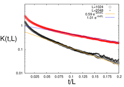
Figure 2: The time evolution of the average number of clusters K(t) for RPM and RPMW. The lines are the expected decays with $K(t,L)\propto e^{-E_{1}t/L}$ with $E_{1}=\frac{2v\pi}{L}$ (RPM) and $E_{1}=\frac{v\pi}{L}$ (RPMW)

IV Avalanches

Figure 3: Example of an even and odd avalanche in RPMW. Avalanches occurring on RPM release only an odd number of tiles

The raise and peel model exhibits events where layers are evaporated from the substrate when a tile from the gas hits the interface. The number of tiles removed defines the size of an avalanche. While this number is always an odd number in RPM, in RPWM there is the possibility of an even number of tiles removed whenever an avalanche touches the boundary. This is illustrated in Figure 3.

It is known that the raise and peel model exhibits self-organized criticality bak ; dhar in the regime for $u\geq 1$ alcaraz . Desorption processes being non–local results in avalanches lacking a characteristic length-scale. Their distribution $S(v,L)$ therefore appears as a power-law which might be described in the finite-size scaling (FSS) form Tebaldi ; Alcaraz0

$$S(v,L)=v^{-\tau}F(\frac{v}{L^{D}})$$ (19)

In order to obtain the exponents, the method of moments is used alcaraz ; Tebaldi . Using the scaling form (Eqn. 19) we have:

$$\langle v^{m}\rangle_{L} =\int S(v,L)v^{m}dv$$ (20)

$$=\int v^{-\tau}F(\frac{v}{L^{D}})v^{m}dv$$ (21)

$$=\int w^{-\tau}L^{-D\tau}F(w)w^{m}w^{mD}L^{D}dw$$ (22)

$$=L^{D(1+m-\tau)}\underbrace{\int w^{m-\tau}F(w)dw}$$ (23)

$$~{}~{}~{}~{}~{}~{}~{}~{}~{}~{}~{}~{}~{}~{}~{}~{}~{}~{}~{}~{}~{}~{}~{}~{}~{}~{}~{}~{}\Gamma_{m}$$ (24)

where we have used $w\equiv v/L^{D}$ to get the scaling dependence with L. We can get an estimate for the exponent by looking at the ratio:

$$\langle v^{m}\rangle_{L}/\langle v^{m}\rangle_{L^{\prime}}=(L/L^{\prime})^{\sigma(m)}$$ (25)

and in this manner the exponent $\sigma(m)$ can be estimated as gier :

$$\sigma(m)=\frac{ln(\langle v^{m}\rangle_{L}/\langle v^{m}\rangle_{L^{\prime}})}{ln(L/L^{\prime})}=\left\{\begin{array}[]{lcl}0&\mbox{for}&m<\tau-1\\ D(1+m-\tau)&\mbox{for}&m>\tau-1\end{array}\right.$$ (26)

A linear fit to Eqn.(26) for $m>\tau-1$ gives an estimate for the values of $D$ and $\tau$. To get an idea of the spread of these values we ran several Monte-Carlo simulations to find the variation of the distribution resulting from different seeds. The results are shown in table 2.

Table 2: Estimates for the critical exponents in $S(v,L)\sim v^{-\tau}F(v/L^{D})$ for even and odd avalanches using lattices L=4096 and L’=8192

	1/u		1.0	0.45	0.005
	RPM alcaraz	odd	1.004	1.026	1.006
D	RPM[this work]	odd	$0.992\pm 0.058$	$1.015\pm 0.006$	$1.006\pm 0.0001$
	RPMW[this work]	odd	$0.994\pm 0.025$	$1.008\pm 0.002$	$1.006\pm 0.0001$
	RPMW[this work]	even	$0.980\pm 0.117$	$1.013\pm 0.008$	$1.006\pm 0.0001$
	RPM alcaraz	odd	3.000	2.25	2.00
$\tau$	RPM[this work]	odd	$2.977\pm 0.079$	$2.224\pm 0.016$	$2.011\pm 0.001$
	RPMW[this work]	odd	$3.003\pm 0.071$	$2.237\pm 0.012$	$2.011\pm 0.001$
	RPMW[this work]	even	$1.932\pm 0.222$	$1.280\pm 0.074$	$1.020\pm 0.011$

Results in this table show that the critical exponents for an odd number of tiles removed remains unchanged by adding a wall. However, we found that for an even number of tiles the power-law exponent $\tau$ decreases by about one. We also found an interesting effect on the finite-size scaling function with the addition of the wall. Fig. 4 shows the scaling function for RPM and RPMW for u=1, where we use $\tau=3.0$ and $\tau=2.0$ respectively, for odd number of tiles and even number of tiles, while D is kept fixed at $D=1$. Fig. 5 shows a similar plot for 1/u=0.005. The data collapse for large lattices on these plots confirms the FSS form (Eqn. 19).

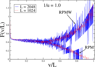
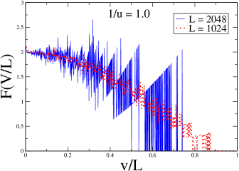
Figure 4: The scaling function $F(\frac{v}{L})$ with rates $1/u=1.0$ for $v\in$ odd number with $\tau=3.0$ and $D=1.0$ (LEFT) and $v\in$ even number with $\tau=2.0$ and $D=1.0$

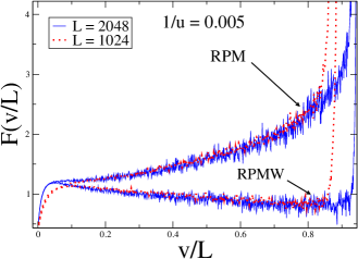
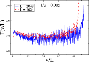
Figure 5: The scaling function $F(\frac{v}{L})$ with rates $1/u=0.005$ for $v\in$ odd number with $\tau=2.0$ and $D=1.0$ (LEFT) and $v\in$ even number with $\tau=1.0$ and $D=1.0$

V Conjectures for Probabilities

Simple conjectures for the probabilities of absorption, desorption, and reflection can be written down by considering the rate of change between the different states. The probability to loose (or gain) v tiles can be written as gier :

$$P(v,L)=\sum_{\eta\neq\eta^{\prime}}\delta(v(\eta^{\prime})-v(\eta)-v)w_{\eta^{\prime}\rightarrow\eta}P_{\eta^{\prime}}/\langle 0|0\rangle$$ (27)

where $P_{\eta^{\prime}}/\langle 0|0\rangle$ is normalized probability to be in the state $|v(\eta^{\prime})\rangle$ (see Eqn. 10) and $w_{\eta^{\prime}\rightarrow\eta}$ is the transition rate $w_{\eta^{\prime}\rightarrow\eta}$ from state $|v(\eta^{\prime})\rangle$ to state $|v(\eta)\rangle$. For u=1, the normalization $\langle 0|0\rangle$ is given by Eqn.(11) and Eqn.(12) for RPM and RPMW, respectively. The probability of absorption ($P_{a}$) for a given L has been given by Alcaraz et al for RPMW Alcaraz2 . In this section we will present new conjectures for the probabilities of desorption ($P_{d}$) and reflection ($P_{r}$) for RPMW. Probabilities for RPM where first reported in gier . These expressions results in quotients of parabolas as seen in table LABEL:table:Probs. Notice the denominator for the probabilities are different with the addition of the wall since normalization expressions for $\langle 0|0\rangle$ (Eqns. 11 and 12) are different for the cases with and without a wall Alcaraz2 .

Table 3: Conjectures for the probabilities of an absorption event $P_{a}\equiv P(-1,L)$, desorption event $P_{d}\equiv P(v>0,L)$, reflection event $P_{r}\equiv P(0,L)$

Prob.gier ; Alcaraz2	$P_{a}$	$P_{d}$	$P_{r}$
RPM ($v\in odd$ )	$\frac{3L(L-2)}{4(2L+1)(L-1)}$	$\frac{2(L-2)(L+2)}{4(2L+1)(L-1)}$	—
RPM ($v\in even$ )	—	—	$\frac{3L^{2}+2L+4}{4(2L+1)(L-1)}$
RPMW ($v\in odd$ )	$\frac{6L^{2}+8L-5}{4(2L+1)(2L+3)}$	$\frac{4L^{2}+5L+9}{4(2L+1)(2L+3)}$	—
RPMW ($v\in even$)	—	$\frac{1.795L-4.562}{4(2L+1)(2L+3)}$	$\frac{6L^{2}+17.211L+12.50}{4(2L+1)(2L+3)}$

It is interesting to note that although this is a non-equilibrium system, simple expressions for probabilities can be obtained. The mean size of an avalanche $\langle v\rangle$ in the stationary state can be conjectured to be given by a mean-field expression alcaraz .

$$\langle v\rangle_{L}=P_{a}(L)/P_{d}(L)$$ (28)

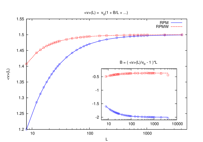
Figure 6: Average avalanche size $\langle v\rangle(L)$ plotted from the ratio of $P_{a}(L)/P_{d}(L)$ (lines) compared to Monte Carlo data for RPM ($\bigcirc$) and RPMW ($\square$)

This is a quotient of parabolas, and in the large limit ($L\gg 1$)

$$\frac{P_{a}(L)}{P_{d}(L)} =\frac{\alpha L^{2}+\beta L+\gamma}{aL^{2}+bL+c}$$

$$=\frac{\alpha L^{2}+\beta L+\gamma}{aL^{2}(1+\frac{b}{aL}+\frac{c}{aL^{2}})}$$

$$\approx(\frac{\alpha}{a}+\frac{\beta}{aL}+\mathcal{O}(L^{-2}))(1-\frac{b}{aL}+\mathcal{O}(L^{-2}))$$

$$\approx(\frac{\alpha}{a}+\frac{\beta}{aL}-\frac{\alpha b}{a^{2}L}+\mathcal{O}(L^{-2}))$$

$$=(\frac{\alpha}{a}+\frac{1}{aL}(\beta-\frac{\alpha b}{a}))$$

$$=\frac{\alpha}{a}(1+\frac{1}{L}(\frac{\beta}{\alpha}-\frac{b}{a}))$$

We assume that $\alpha\neq 0$ and $a\neq 0$ and dropped terms of the order of $\mathcal{O}(L^{-2}))$. From Table LABEL:table:Probs we see that for RPM we have

$$\frac{P_{a}(L)}{P_{d}(L)} =\frac{3}{2}(1-\frac{1}{L}(\frac{6}{3}-\frac{0}{2}))$$

$$\Rightarrow\langle v\rangle_{L} =\frac{3}{2}(1-\frac{2}{L})$$

while for RPMW we have:

$$\frac{P_{a}(L)}{P_{d}(L)} =\frac{6}{4}(1+\frac{1}{L}(\frac{8}{6}-\frac{6.795}{4}))$$

$$\Rightarrow\langle v\rangle_{L} =\frac{3}{2}(1-\frac{0.365}{L})$$

The estimated average from the ratio of the conjectures agrees quite well as can be seen in Fig 6. This remarkable since this describes a non-equilibrium system.

It is interesting to see that the leading term on this expansion is universal, whereas the correction term depends on the details of the model (i.e. whether there is a wall or not). This is a similar behavior as in finite–size scaling of the concentration of particles in certain reaction–diffusion systems birgit1 ; birgit2 ; birgit3 and surface exponent corrections to quantum chains using different types of boundary conditions alcaraz_surface ; Turban ; BX .

The simple functional form for the probabilities shown in table LABEL:table:Probs suggests we can guess a general quadratic expression in L for the probabilities P(v,L) by fixing the denominator as:

$$P_{RPM}(v,L)=\frac{a(v)L^{2}+b(v)L+c(v)}{4(2L+1)(L-1)}$$ (32)

$$P_{RPMW}(v,L)=\frac{a(v)L^{2}+b(v)L+c(v)}{4(2L+3)(2L+1)}$$ (33)

and fitting for the parameters {$a(v)$, $b(v)$, $c(v)$} in the forms (32) and (33). The behavior of these parameters with respect to $v$ is shown in Fig 7. As expected, the quadratic term shows a power-law behavior $\propto v^{-3.0}$. The linear and constant terms however do show different behavior, but we were not able to reduce it to an analytical form.

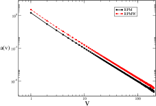
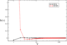
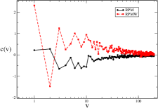
Figure 7: Behavior of the quadratic term $a(v)$, linear term $b(v)$ and constant term $c(v)$ obtained from fits to Eqn. 32 and Eqn. 33.

Consistency on the fits demands that (see table LABEL:table:Probs)

$$\sum_{v>0}P_{RPM}(v,L)=\frac{2L^{2}+0L-8}{4(2L+1)(L-1)}$$ (34)

$$\sum_{v>0}P_{RPMW}(v,L)=\frac{4L^{2}+5L+9}{4(2L+3)(2L+1)}$$ (35)

The sums over the parameters $\sum_{v}$ {$a(v),b(v),c(v)$} are shown in Table 4 for RPM and RPMW. We see that the quadratic $a(v)$ and linear $b(v)$ terms capture the behavior in $v$ quite well, whereas as shown in Fig 7 the constant term $c(v)$ is dominated by fluctuations on the fits.

	$\sum_{v}a(v)$	$\sum_{v}b(v)$	$\sum_{v}c(v)$
RPM	1.99999	-0.00375	-13.8002
RPMW	3.99997	4.96604	30.4445

Table 4: Sums over $v$ for the parameters resulting from the fits

VI conclusion

We studied the non-equilibrium statistical model known as the raise and peel model. We have confirmed that this model retains several features as predicted from conformal invariance for stochastic profiles characterizing the system when changing the boundary conditions. We allowed one boundary to fluctuate and demonstrated that the temporal profile of a stochastic quantity follows its expected behavior from stochastic dynamics where the long time behavior is dominated by the lowest non-zero eigenvalue. We study the surface dynamics by looking at avalanche distributions exhibiting power-law distributions. Using the finite-size scaling formalism we confirm the universality exponent $\tau=3.0$ for the Raise and Peel with different boundary conditions and we identified an even/odd effect with a new exponent $\tau=2.0$ for avalanches with an even number of tiles removed. We also found new conjectures for the probability of desorption and reflection with a wall added to the system and checked that they agree with Monte Carlo data.

Acknowledgements

We would like to thank M. Henkel and the Groupe de Physique Statistique at Nancy University for helpful discussions. B. W.-K. thankfully acknowledges support from the NSF under the grant PHY-0969689.

References

• (1) P. A. Pearce J. de Gier, B. Nienhuis and V. Rittenberg. Stochastic processes and conformal invariance. Phys. Rev. E, 67:016101, 2003.
• (2) P. A. Pearce J. de Gier, B. Nienhuis and V. Rittenberg. The raise and peel model of a fluctuating interface. Journal of Statistical Physics, 114:1–35, 2004.
• (3) F. C. Alcaraz, M. Droz, M. Henkel, and V. Rittenberg. Reaction-Diffusion Processes, Critical Dynamics, and Quantum Chains. Annals of Physics, 230(2):250–302, 1994.
• (4) F. C. Alcaraz, E. Levine, and V. Rittenberg. Conformal invariance and its breaking in a stochastic model of a fluctuating interface. Journal of Statistical Mechanics: Theory and Experiment, 2006(08):P08003, 2006.
• (5) F. C. Alcaraz and V. Rittenberg. Different facets of the raise and peel model. Journal of Statistical Mechanics: Theory and Experiment, 2007(07):P07009, 2007.
• (6) P. Bak, C. Tang, and K. Wiesenfeld. Self-organized criticality. Phys. Rev. A, 38:364–374, 1988.
• (7) D. Dhar. Studying Self-Organized Criticality with Exactly Solved Models. Prerint arXiv:cond-mat/9909009, 1999.
• (8) A. V. Razumov and Yu G. Stroganov. Spin chains and combinatorics. Journal of Physics A: Mathematical and General, 34(14):3185+, 2001.
• (9) A. V. Razumov and Yu. G. Stroganov. Spin chains and combinatorics: twisted boundary conditions. Journal of Physics A: Mathematical and General, 34(26):5335, 2001.
• (10) J. de Gier. The razumovstroganov conjecture: stochastic processes, loops and combinatorics. Journal of Statistical Mechanics: Theory and Experiment, 2007(02):N02001, 2007.
• (11) J. de Gier M. T. Batchelor and B. Nienhuis. The quantum symmetric xxz chain at $\delta=\frac{-1}{2}$, alternating-sign matrices and plane partitions. Journal of Physics A: Mathematical and General, 34(19):L265, 2001.
• (12) F. C. Alcaraz and M. J. Martins. Conformal invariance and the operator content of the xxz model with arbitrary spin. Journal of Physics A: Mathematical and General, 22(11):1829, 1989.
• (13) International Summer School on Fundamental Problems in Statistical Mechanics and H. van Beijeren. Fundamental problems in statistical mechanics VII : proceedings of the Seventh International Summer School on Fundamental Problems in Statistical Mechanics, Altenburg, F.R. Germany, June 18-30, 1989 / editor, H. Van Beijeren. North-Holland ; Elsevier Science Pub. Co., Amsterdam ; New York, 1990.
• (14) M. Henkel. Conformal Invariance and Critical Phenomena. Springer, 1999.
• (15) F. C. Alcaraz, P. Pyatov, and V. Rittenberg. Density profiles in the raise and peel model with and without a wall; physics and combinatorics. Journal of Statistical Mechanics: Theory and Experiment, 2008(01):P01006, 2008.
• (16) P. Pyatov. Raise and peel models of fluctuating interfaces and combinatorics of pascal’s hexagon. Journal of Statistical Mechanics: Theory and Experiment, 2004(09):P09003, 2004.
• (17) F. C. Alcaraz and V. Rittenberg. Reaction-diffusion processes as physical realizations of hecke algebras. Physics Letters B, 314(3):377 – 380, 1993.
• (18) O. Golinelli and K. Mallick. The asymmetric simple exclusion process: an integrable model for non-equilibrium statistical mechanics. Journal of Physics A: Mathematical and General, 39(41):12679, 2006.
• (19) J. de Gier P. A. Pearce, V. Rittenberg and B. Nienhuis. Temperley-Lieb stochastic processes. Journal of Physics A: Mathematical and General, 35(45):L661, 2002.
• (20) A Nichols, V Rittenberg, and J de Gier. One-boundary temperley–lieb algebras in the xxz and loop models. Journal of Statistical Mechanics: Theory and Experiment, 2005(03):P03003, 2005.
• (21) J. de Gier and V. Rittenberg. Refined razumov-stroganov conjectures for open boundaries. Journal of Statistical Mechanics: Theory and Experiment, 2004(09):P09009, 2004.
• (22) S. Mitra, B. Nienhuis, J. de Gier, and M. T. Batchelor. Exact expressions for correlations in the ground state of the dense o(1) loop model. Journal of Statistical Mechanics: Theory and Experiment, 2004(09):P09010, 2004.
• (23) J. de Gier. Loops, matchings and alternating-sign matrices. Discrete Mathematics, 298(1–3):365 – 388, 2005.
• (24) J. Propp. The many faces of alternating-sign matrices. Discrete Mathematics and Theoretical Computer Science Proceedings AA (DM-CCG), pages 43+, 2001.
• (25) P.A. Pearce, V. Rittenberg, and J. de Gier. Critical q=1 potts model and temperley-lieb stochastic processes. Preprint arXiv:cond-mat/0108051, 2001.
• (26) J. de Gier, A. Nichols, P. Pyatov, and V. Rittenberg. Magic in the spectra of the xxz quantum chain with boundaries at and. Nuclear Physics B, 729(3):387 – 418, 2005.
• (27) X. Yang and P. Fendley. Non-local spacetime supersymmetry on the lattice. Journal of Physics A: Mathematical and General, 37:8937, 2004.
• (28) F. Family and T. Vicsek. Scaling of the active zone in the eden process on percolation networks and the ballistic deposition model. Journal of Physics A: Mathematical and General, 18(2):L75, 1985.
• (29) C. Tebaldi, M. De Menech, and A. L. Stella. Multifractal scaling in the bak-tang-wiesenfeld sandpile and edge events. Phys. Rev. Lett., 83:3952–3955, 1999.
• (30) K. Krebs, M. Pfannmüller, B. Wehefritz, and H. Hinrichsen. Finite-size scaling studies of one-dimensional reaction-diffusion systems. part i. analytical results. Journal of Statistical Physics, 78:1429–1470, 1995.
• (31) K. Krebs, M. Pfannmüller, H. Simon, and B. Wehefritz. Finite-size scaling studies of one-dimensional reaction-diffusion systems. part ii. numerical methods. Journal of Statistical Physics, 78:1471–1491, 1995.
• (32) U. Bilstein and B. Wehefritz. The xx-model with boundaries: Part i. diagonalization of the finite chain. Journal of Physics A: Mathematical and General, 32(2):191, 1999.
• (33) F. C. Alcaraz, M. N. Barber, M. T. Batchelor, R. J. Baxter, and G. R. W. Quispel. Surface exponents of the quantum xxz, ashkin-teller and potts models. Journal of Physics A: Mathematical and General, 20(18):6397, 1987.
• (34) L. Turban and F. Igli. Off-diagonal density profiles and conformal invariance. Journal of Physics A: Mathematical and General, 30(5):L105, 1997.
• (35) T. W. Burkhardt and T. Xue. Density profiles in confined critical systems and conformal invariance. Phys. Rev. Lett., 66:895–898, 1991.