Which electric fields are realizable in conducting materials?

Abstract

In this paper we study the realizability of a given smooth periodic gradient field $\nabla u$ defined in $\mathbb{R}^{d}$, in the sense of finding when one can obtain a matrix conductivity $\sigma$ such that $\sigma\nabla u$ is a divergence free current field. The construction is shown to be always possible locally in $\mathbb{R}^{d}$ provided that $\nabla u$ is non-vanishing. This condition is also necessary in dimension two but not in dimension three. In fact the realizability may fail for non-regular gradient fields, and in general the conductivity cannot be both periodic and isotropic. However, using a dynamical systems approach the isotropic realizability is proved to hold in the whole space (without periodicity) under the assumption that the gradient does not vanish anywhere. Moreover, a sharp condition is obtained to ensure the isotropic realizability in the torus. The realizability of a matrix field is also investigated both in the periodic case and in the laminate case. In this context the sign of the matrix field determinant plays an essential role according to the space dimension.

Marc Briane,  Graeme W. Milton,  Andrejs Treibergs

Keywords : Conductivity, Electric field, Dynamical systems

Mathematics Subject Classification : 35B27, 78A30, 37C10

1 Introduction

The mathematical study of composite media has grown remarkably since the seventies through the asymptotic analysis of pde’s governing their behavior (see, e.g., [6], [5], [12], [14]). In the periodic framework of the conductivity equation, the derivation of the effective (or homogenized) properties of a given composite conductor in $\mathbb{R}^{d}$, with a periodic matrix-valued conductivity $\sigma$, reduces to the cell problem of finding periodic gradients $\nabla u$ solving

$$\mbox{\rm div}\left(\sigma\nabla u\right)=0\quad\mbox{in }\mathbb{R}^{d},$$ (1.1)

which gives the effective conductivity $\sigma^{*}$ via the average formula

$$\sigma^{*}\langle\nabla u\rangle=\langle\sigma\nabla u\rangle.$$ (1.2)

Note that the periodicity condition is not actually a restriction, since by [17] (see also [2], Theorem 1.3.23) any effective matrix can be shown to be a pointwise limit of a sequence of periodic homogenized matrices. In equation (1.1) the vector-valued function $\nabla u$ represents the electric field, while $\sigma\nabla u$ is the current field according to Ohm’s law. Alternatively we can consider a vector-valued potential $U$ with gradient $DU$ where each component of $U$ satisfies (1.1). In this case the components of $U$ represent the potentials obtained for different applied fields, and $DU$ will be referred to as the matrix-valued electric field. Going back to the original conductivity problem it is then natural to characterize mathematically among all periodic gradient fields those solving the conductivity equation (1.1) for some positive definite symmetric periodic matrix-valued function $\sigma$. In other words the question is to know which electric fields are realizable. On the other hand, this work is partly motivated by the search for sharp bounds on the effective moduli of composites. This search has led investigators to derive as much information as possible about fields in composites. A prime example is given by the positivity of the determinant of periodic matrix-valued electric fields in two dimensions obtained by Alessandrini and Nesi [1]. This led to sharp bounds on effective moduli for three phase conducting composites (see, e.g., [16, 10]). Therefore, a natural question to ask, which we address here, is: what are the conditions on a gradient to be realizable as an electric field?

In Section 2 we focus on vector-valued electric fields. First of all, due to the rectification theorem we prove (see Theorem 2.2) that any non-vanishing smooth gradient field $\nabla u$ is isotropically realizable locally in $\mathbb{R}^{d}$, in the sense that in the neighborhood of each point equation (1.1) holds for some isotropic conductivity $\sigma I_{d}$. Two examples show that the regularity of the gradient field is essential, and that the periodicity of $\sigma$ is not satisfied in general. Conversely, in dimension two the realizability of a smooth periodic gradient field $\nabla u$ implies that $\nabla u$ does not vanish in $\mathbb{R}^{2}$. This is not the case in dimension three as exemplified by the periodic chain-mail of [8]. Again in dimension two a necessary and sufficient condition for the (at least anisotropic) realizability is given (see Theorem 2.7). Then, the question of the global isotropic realizability is investigated through a dynamical systems approach. On the one hand, considering the trajectories along the gradient field $\nabla u$ which cross a fixed hyperplane, we build (see Proposition 2.10) an admissible isotropic conductivity $\sigma$ in the whole space. The construction is illustrated with the potential $u(x):=x_{1}-\cos(2\pi x_{2})$ in dimension two. On the other hand, upon replacing the hyperplane by the equipotential $\{u=0\}$, a general formula for the isotropic conductivity $\sigma$ is derived (see Theorem 2.14) for any smooth gradient field in $\mathbb{R}^{d}$. Finally, a sharp condition for the isotropic realizability in the torus is obtained (see Theorem 2.16), which allows us to construct a periodic conductivity $\sigma$.

Section 3 is devoted to matrix-valued fields. The goal is to characterize those smooth potentials $U=(u_{1},\dots,u_{d})$ the gradient $DU$ of which is a realizable periodic matrix-valued electric field. When the determinant of $DU$ has a constant sign, it is proved to be realizable with an anisotropic matrix-valued conductivity $\sigma$. This can be achieved in an infinite number of ways using Piola’s identity coming from mechanics (see Theorem 3.2 and Proposition 3.5). This yields a necessary and sufficient realizability condition in dimension two due to the determinant positivity result of [1]. However, the periodic chain-mail example of [8] shows that this condition is not necessary in dimension three. We extend (see Theorem 3.7) the realizability result to (non-regular) laminate matrix fields having the remarkable property of a constant sign determinant in any dimension (see [8], Theorem 3.3).

Notations

• $\left(e_{1},\dots,e_{d}\right)$ denotes the canonical basis of $\mathbb{R}^{d}$.

• $I_{d}$ denotes the unit matrix of $\mathbb{R}^{d\times d}$, and $R_{\perp}$ denotes the $90^{\circ}$ rotation matrix in $\mathbb{R}^{2\times 2}$.

• For $A\in\mathbb{R}^{d\times d}$, $A^{T}$ denotes the transpose of the matrix $A$.

• For $\xi,\eta\in\mathbb{R}^{d}$, $\xi\otimes\eta$ denotes the matrix $\left[\xi_{i}\,\eta_{j}\right]_{1\leq i,j\leq d}$.

• $Y$ denotes any closed parallelepiped of $\mathbb{R}^{d}$, and $Y_{d}:=\left[0,1\right]^{d}$.

• $\langle\cdot\rangle$ denotes the average over $Y$.

• $C^{k}_{\sharp}(Y)$ denotes the space of $k$-continuously differentiable $Y$-periodic functions on $\mathbb{R}^{d}$.

• $L^{2}_{\sharp}(Y)$ denotes the space of $Y$-periodic functions in $L^{2}(\mathbb{R}^{d})$, and $H^{1}_{\sharp}(Y)$ denotes the space of functions $\varphi\in L^{2}_{\sharp}(Y)$ such that $\nabla\varphi\in L^{2}_{\sharp}(Y)^{d}$.

• For any open set $\Omega$ of $\mathbb{R}^{d}$, $C^{\infty}_{c}(\Omega)$ denotes the space of smooth functions with compact support in $\Omega$, and $\mathscr{D}^{\prime}(\Omega)$ the space of distributions on $\Omega$.

• For $u\in C^{1}(\mathbb{R}^{d})$ and $U=(U_{j})_{1\leq j\leq d}\in C^{1}(\mathbb{R}^{d})^{d}$,

  $$\nabla u:=\left({\partial u\over\partial x_{i}}\right)_{1\leq i\leq d}\quad\mbox{and}\quad DU:=\big{(}\nabla U_{1},\dots,\nabla U_{d}\big{)}=\left[{\partial U_{j}\over\partial x_{i}}\right]_{1\leq i,j\leq d}.$$ (1.3)

  The partial derivative $\displaystyle{\partial u\over\partial x_{i}}$ will be sometimes denoted $\partial_{i}u$.

• For $\Sigma=\left[\Sigma_{ij}\right]_{1\leq i,j\leq d}\in C^{1}(\mathbb{R}^{d})^{d\times d}$,

  $$\mbox{\rm Div}\left(\Sigma\right):=\left(\sum_{i=1}^{d}{\partial\Sigma_{ij}\over\partial x_{i}}\right)_{1\leq j\leq d}\quad\mbox{and}\quad\mbox{\rm Curl}\left(\Sigma\right):=\left({\partial\Sigma_{ik}\over\partial x_{j}}-{\partial\Sigma_{jk}\over\partial x_{i}}\right)_{1\leq i,j,k\leq d}.$$ (1.4)

• For $\xi^{1}_{1},\dots,\xi^{d-1}$ in $\mathbb{R}^{d}$, the cross product $\xi^{1}\times\cdots\times\xi^{d-1}$ is defined by

  $$\xi\cdot\left(\xi^{1}\times\cdots\times\xi^{d-1}\right)=\det\left(\xi,\xi^{1},\dots,\xi^{d-1}\right),\quad\mbox{for any }\xi\in\mathbb{R}^{d},$$ (1.5)

  where $\det$ is the determinant with respect to the canonical basis $(e_{1},\dots,e_{d})$, or equivalently, the $k^{\rm th}$ coordinate of the cross product is given by

  $$\left(\xi^{1}\times\cdots\times\xi^{d-1}\right)\cdot e_{k}=(-1)^{k+1}\left|\,\begin{smallmatrix}\xi^{1}_{1}&\cdots&\xi^{d-1}_{1}\\ \vdots&\qquad\ddots\qquad&\vdots\\ \\ \xi^{1}_{k-1}&\cdots&\xi^{d-1}_{k-1}\\ \xi^{1}_{k+1}&\cdots&\xi^{d-1}_{k+1}\\ \vdots&\qquad\ddots\qquad&\vdots\\ \\ \xi^{1}_{d}&\cdots&\xi^{d-1}_{d}\end{smallmatrix}\,\right|.$$ (1.6)

2 The vector field case

Definition 2.1.

Let $\Omega$ be an (bounded or not) open set of $\mathbb{R}^{d}$, $d\geq 2$, and let $u\in H^{1}(\Omega)$. The vector-valued field $\nabla u$ is said to be a realizable electric field in $\Omega$ if there exist a symmetric positive definite matrix-valued $\sigma\in L^{\infty}_{\rm loc}(\Omega)^{d\times d}$ such that

$$\mbox{\rm div}\left(\sigma\nabla u\right)=0\quad\mbox{in }\mathscr{D}^{\prime}(\Omega).$$ (2.1)

If $\sigma$ can be chosen isotropic ($\sigma\to\sigma I_{d}$), the field $\nabla u$ is said to be isotropically realizable in $\Omega$.

2.1 Isotropic and anisotropic realizability

2.1.1 Characterization of an isotropically realizable electric field

Theorem 2.2.

Let $Y$ be a closed parallelepiped of $\mathbb{R}^{d}$. Consider $u\in C^{1}(\mathbb{R}^{d})$, $d\geq 2$, such that

$$\nabla u\mbox{ is $Y$-periodic}\quad\mbox{and}\quad\langle\nabla u\rangle\neq 0.$$ (2.2)

• Assume that

  $$\nabla u\neq 0\quad\mbox{everywhere in }\mathbb{R}^{d}.$$ (2.3)

  Then, $\nabla u$ is an isotropically realizable electric field locally in $\mathbb{R}^{d}$ associated with a continuous conductivity.

• Assume that $\nabla u$ satisfies condition (2.2), and is a realizable electric field in $\mathbb{R}^{2}$ associated with a smooth $Y$-periodic conductivity. Then, condition (2.3) holds true.

• There exists a gradient field $\nabla u$ satisfying (2.2), which is a realizable electric field in $\mathbb{R}^{3}$ associated with a smooth $Y_{3}$-periodic conductivity, and which admits a critical point $y_{0}$, i.e. $\nabla u(y_{0})=0$.

Remark 2.3.

Part $i)$ of Theorem 2.2 provides a local result in the smooth case, and still holds without the periodicity assumption on $\nabla u$. It is then natural to ask if the local result remains valid when the potential $u$ is only Lipschitz continuous. The answer is negative as shown in Example 2.4 below. We may also ask if a global realization of a periodic gradient can always be obtained with a periodic isotropic conductivity $\sigma$. The answer is still negative as shown in Example 2.6.

The underlying reason for these negative results is that the proof of Theorem 2.2 is based on the rectification theorem which needs at least $C^{1}$-regularity and is local.

Example 2.4.

Let $\chi:\mathbb{R}\to\mathbb{R}$ be the $1$-periodic characteristic function which agrees with the characteristic function of $[0,1/2]$ on $[0,1]$. Consider the function $u$ defined in $\mathbb{R}^{2}$ by

$$u(x):=x_{2}-x_{1}+\int_{0}^{x_{1}}\chi(t)\,dt,\quad\mbox{for any }x=(x_{1},x_{2})\in\mathbb{R}^{2}.$$ (2.4)

The function $u$ is Lipschitz continuous, and

$$\nabla u=\chi\,e_{2}+\left(1-\chi\right)\left(e_{2}-e_{1}\right)\quad\mbox{a.e. in }\in\mathbb{R}^{2}.$$ (2.5)

The discontinuity points of $\nabla u$ lie on the lines $\{x_{1}=1/2\left(1+k\right)\}$, $k\in\mathbb{Z}$. Let $Q:=(-r,r)^{2}$ for some $r\in(0,1/2)$.

Assume that there exists a positive function $\sigma\in L^{\infty}(Q)$ such that $\sigma\nabla u$ is divergence free in $Q$. Let $v$ be a stream function such that $\sigma\nabla u=R_{\perp}\nabla v$ a.e. in $Q$. The function $v$ is unique up to an additive constant, and is Lipschitz continuous. On the one hand, we have

$$0=\nabla u\cdot\nabla v=(e_{2}-e_{1})\cdot\nabla v\quad\mbox{a.e. in }(-r,0)\times(-r,r),$$ (2.6)

hence $v(x)=f(x_{1}+x_{2})$ for some Lipschitz continuous function $f$ defined in $[-2r,r]$. On the other hand, we have

$$0=\nabla u\cdot\nabla v=e_{2}\cdot\nabla v\quad\mbox{a.e. in }(0,r)\times(-r,r),$$ (2.7)

hence $v(x)=g(x_{1})$ for some Lipschitz continuous function $g$ in $[0,r]$. By the continuity of $v$ on the line $\{x_{1}=0\}$, we get that $f(x_{2})=g(0)$, hence $f$ is constant in $[-r,r]$. Therefore, we have

$$\nabla v=0\;\;\mbox{a.e. in }(-r,0)\times(0,r)\quad\mbox{and}\quad\sigma\nabla u=\sigma\left(e_{2}-e_{1}\right)\neq 0\;\;\mbox{a.e. in }(-r,0)\times(0,r),$$ (2.8)

which contradicts the equality $\sigma\nabla u=R_{\perp}\nabla v$ a.e. in $Q$. Therefore, the field $\nabla u$ is non-zero a.e. in $\mathbb{R}^{2}$, but is not an isotropically realizable electric field in the neighborhood of any point of the lines $\{x_{1}=1/2\left(1+k\right)\}$, $k\in\mathbb{Z}$.

Remark 2.5.

The singularity of $\nabla u$ in Example 2.4 induces a jump of the current at the interface $\{x_{1}=0\}$. To compensate this jump we need to introduce formally an additional current concentrated on this line, which would imply an infinite conductivity there. The assumption of bounded conductivity (in $L^{\infty}$) leads to the former contradiction. Alternatively, with a smooth approximation of $\nabla u$ around the line $\{x_{1}=0\}$, then part $i)$ of Theorem 2.2 applies which allows us to construct a suitable conductivity. But this conductivity blows up as the smooth gradient tends to $\nabla u$.

Example 2.6.

Consider the function $u$ defined in $\mathbb{R}$ by

$$u(x):=x_{1}-\cos\left(2\pi x_{2}\right),\quad\mbox{for any }x=(x_{1},x_{2})\in\mathbb{R}^{2}.$$ (2.9)

The function $u$ is smooth, and its gradient $\nabla u$ is $Y_{2}$-periodic, independent of the variable $x_{1}$ and non-zero on $\mathbb{R}^{2}$.

Assume that there exists a smooth positive function $\sigma$ defined in $\mathbb{R}^{2}$, which is $a$-periodic with respect to $x_{1}$ for some $a>0$, and such that $\sigma\nabla u$ is divergence free in $\mathbb{R}^{2}$. Set $Q:=(0,a)\times(-r,r)$ for some $r\in(0,{1\over 2})$. By an integration by parts and taking into account the periodicity of $\sigma\nabla u$ with respect to $x_{1}$, we get that

$$\begin{array}[]{ll}\displaystyle 0&\displaystyle=\int_{Q}\mbox{\rm div}\left(\sigma\nabla u\right)dx\\ \vskip 6.0pt plus 2.0pt minus 2.0pt\cr&\displaystyle=\underbrace{\int_{-r}^{r}\big{(}\sigma\nabla u(a,x_{2})-\sigma\nabla u(0,x_{2})\big{)}\cdot e_{1}\,dx_{2}}_{=0}+\int_{0}^{a}\big{(}\sigma\nabla u(x_{1},r)-\sigma\nabla u(x_{1},-r)\big{)}\cdot e_{2}\,dx_{1}\\ &\displaystyle=2\pi\sin\left(2\pi r\right)\int_{0}^{a}\big{(}\sigma(x_{1},r)+\sigma(x_{1},-r)\big{)}\,dx_{1}>0,\end{array}$$ (2.10)

which yields a contradiction. Therefore, the $Y_{2}$-periodic field $\nabla u$ is not an isotropically realizable electric field in the torus.

Proof of Theorem 2.2.

$i)$ Let $x_{0}\in\mathbb{R}^{d}$. First assume that $d>2$. By the rectification theorem (see, e.g., [4]) there exist an open neighborhood $V_{0}$ of $x_{0}$, an open set $W_{0}$, and a $C^{1}$-diffeomorphism $\Phi:V_{0}\to W_{0}$ such that $D\Phi^{T}\,\nabla u=e_{1}$. Define $v_{i}:=\Phi_{i+1}$ for $i\in\{1,\dots,d-1\}$. Then, we get that $\nabla v_{i}\cdot\nabla u=0$ in $V_{0}$, and the rank of $(\nabla v_{1},\dots,\nabla v_{d-1})$ is equal to $(d-1)$ in $V_{0}$. Consider the continuous function

$$\sigma:={|\nabla v_{1}\times\cdots\times\nabla v_{d-1}|\over|\nabla u|}>0\quad\mbox{in }V_{0}.$$ (2.11)

Since by definition, the cross product $\nabla v_{1}\times\cdots\times\nabla v_{d-1}$ is orthogonal to each $\nabla v_{i}$ as is $\nabla u$, then due to the condition (2.3) combined with a continuity argument, there exists a fixed $\tau_{0}\in\{\pm 1\}$ such that

$$\nabla v_{1}\times\cdots\times\nabla v_{d-1}=\tau_{0}\,\sigma\nabla u\quad\mbox{in }V_{0}.$$ (2.12)

Moreover, Theorem 3.2 of [11] implies that $\nabla v_{1}\times\cdots\times\nabla v_{d-1}$ is divergence free, and so is $\sigma\nabla u$. Therefore, $\nabla u$ is an isotropically realizable electric field in $V_{0}$.

When $d=2$, the equality $\nabla v_{1}\cdot\nabla u=0$ in $V_{0}$ yields for some fixed $\tau_{0}\in\{\pm 1\}$,

$$\tau_{0}\,R_{\perp}\nabla v_{1}=\underbrace{{|\nabla v_{1}|\over|\nabla u|}}_{\textstyle\sigma:=}\nabla u\quad\mbox{in }V_{0},$$ (2.13)

which also allows us to conclude the proof of $(i)$.

$ii)$ It is a straightforward consequence of [1] (Proposition 2, the smooth case).

$iii)$ Ancona [3] first built an example of potential with critical points in dimension $d\geq 3$. The following construction is a regularization of the simpler example of [8] which allows us to derive a change of sign for the determinant of the matrix electric field. Consider the periodic chain-mail $Q_{\sharp}\subset\mathbb{R}^{3}$ of [8], and the associated isotropic two-phase conductivity $\sigma^{\kappa}$ which is equal to $\kappa\gg 1$ in $Q_{\sharp}$ and to $1$ elsewhere. Now, let us modify slightly the conductivity $\sigma^{\kappa}$ by considering a smooth $Y_{3}$-periodic isotropic conductivity $\tilde{\sigma}^{\kappa}\in[1,\kappa]$ which agrees with $\sigma^{\kappa}$, except within a thin boundary layer of each interlocking ring $Q\subset Q_{\sharp}$, of width $\kappa^{-1}$ from the boundary of $Q$. Proceeding as in [8] it is easy to prove that the smooth periodic matrix-valued electric field $D\tilde{U}^{\kappa}$ solution of

$$\mbox{\rm Div}\,\big{(}\tilde{\sigma}^{\kappa}D\tilde{U}^{\kappa}\big{)}=0\;\;\mbox{in }\mathbb{R}^{3},\quad\mbox{with}\quad\langle D\tilde{U}^{\kappa}\rangle=I_{3},$$ (2.14)

converges (as $\kappa\to\infty$) strongly in $L^{2}(Y_{3})^{3\times 3}$ to the same limit $DU$ as the electric field $DU^{\kappa}$ associated with $\sigma^{\kappa}$. Then, by virtue of [8] $\det\left(DU\right)$ is negative around some point between two interlocking rings, so is $\det\big{(}D\tilde{U}^{\kappa}\big{)}$ for $\kappa$ large enough. This combined with $\big{\langle}\det\big{(}D\tilde{U}^{\kappa}\big{)}\big{\rangle}=1$ and the continuity of $D\tilde{U}^{\kappa}$, implies that there exists some point $y_{0}\in Y_{3}$ such that $\det\big{(}D\tilde{U}^{\kappa}(y_{0})\big{)}=0$. Therefore, there exists $\xi\in\mathbb{R}^{3}\setminus\{0\}$ such that the potential $u:=\tilde{U}^{\kappa}\cdot\xi$ satisfies $\langle\nabla u\rangle=\xi$ and $\nabla u(y_{0})=D\tilde{U}^{\kappa}(y_{0})\,\xi=0$. Theorem 2.2 is thus proved. $\Box$

2.1.2 Characterization of the anisotropic realizability in dimension two

In dimension two we have the following characterization of realizable electric vector fields:

Theorem 2.7.

Let $Y$ be a closed parallelogram of $\mathbb{R}^{2}$. Consider a function $u\in C^{1}(\mathbb{R}^{2})$ satisfying (2.2). Then, a necessary and sufficient condition for $\nabla u$ to be a realizable electric field associated with a symmetric positive definite matrix-valued conductivity in $C^{0}_{\sharp}(Y)^{d\times d}$, is that there exists a function $v\in C^{1}(\mathbb{R}^{2})$ satisfying (2.2) such that

$$R_{\perp}\nabla u\cdot\nabla v=\det\left(\nabla u,\nabla v\right)>0\quad\mbox{everywhere in }\mathbb{R}^{2}.$$ (2.15)

Remark 2.8.

The result of Theorem 2.7 still holds under the less regular assumption

$$\nabla u\in L^{2}_{\sharp}(Y)^{2},\quad\nabla u\neq 0\;\;\mbox{everywhere in }\mathbb{R}^{2}\quad\mbox{and}\quad\langle\nabla u\rangle\neq 0.$$ (2.16)

Then, the $Y$-periodic conductivity $\sigma$ defined by the formula (2.17) below is only defined almost everywhere in $\mathbb{R}^{2}$, and is not necessarily uniformly bounded from below or above in the cell period $Y$. However, $\sigma\nabla u$ remains divergence free in the sense of distributions on $\mathbb{R}^{2}$.

Proof of Theorem 2.7.

Sufficient condition: Let $u,v\in C^{1}(\mathbb{R}^{2})$ be two functions satisfying (2.2) and (2.15). From (2.15) we easily deduce that $\nabla u$ does not vanish in $\mathbb{R}^{2}$. Then, we may define in $\mathbb{R}^{2}$ the function

$$\sigma:={1\over|\nabla u|^{4}}\begin{pmatrix}\partial_{1}u&\partial_{2}u\\ -\partial_{2}u&\partial_{1}u\end{pmatrix}^{T}\begin{pmatrix}R_{\perp}\nabla u\cdot\nabla v&-\nabla u\cdot\nabla v\\ -\nabla u\cdot\nabla v&{|\nabla u\cdot\nabla v|^{2}+1\over R_{\perp}\nabla u\cdot\nabla v}\end{pmatrix}\begin{pmatrix}\partial_{1}u&\partial_{2}u\\ -\partial_{2}u&\partial_{1}u\end{pmatrix}.$$ (2.17)

Hence, $\sigma$ is a symmetric positive definite matrix-valued function in $C^{0}_{\sharp}(Y)^{d\times d}$ with determinant $|\nabla u|^{-4}$. Moreover, a simple computation shows that $\sigma\nabla u=-\,R_{\perp}\nabla v$, so that $\sigma\nabla u$ is divergence free in $\mathbb{R}^{d}$. Therefore, $\nabla u$ is a realizable electric field in $\mathbb{R}^{d}$ associated with the anisotropic conductivity $\sigma$.

Necessary condition: Let $u\in C^{1}(\mathbb{R})$ satisfying (2.2) such that $\nabla u$ is a realizable electric field associated with a symmetric positive definite matrix-valued conductivity $\sigma\in C^{0}_{\sharp}(Y)^{d\times d}$ in $\mathbb{R}^{d}$. Consider the unique (up to an additive constant) potential $v$ which solves $\mbox{\rm div}\left(\sigma\nabla v\right)=0$ in $\mathbb{R}^{d}$, with $\nabla v\in H^{1}_{\sharp}(Y)^{d}$ and $\langle\nabla v\rangle=R_{\perp}\,\langle\nabla u\rangle$, and set $U:=(u,v)$. By (2.2) we have

$$\det\big{(}\langle DU\rangle\big{)}=R_{\perp}\langle\nabla u\rangle\cdot\langle\nabla v\rangle=\big{|}\langle\nabla u\rangle\big{|}^{2}>0.$$ (2.18)

Hence, due to [1] (Theorem 1) we have $\det\left(DU\right)>0$ a.e. in $\mathbb{R}^{2}$. On the other hand, assume that there exists a point $y_{0}\in\mathbb{R}^{2}$ such that $\det\left(DU\right)(y_{0})=0$. Then, there exists $\xi\in\mathbb{R}^{2}\setminus\{0\}$ such that the potential $u:=U\xi$ satisfies $\nabla u(y_{0})=DU(y_{0})\,\xi=0$, which contradicts Proposition 2 of [1] (the smooth case). Therefore, we get that $R_{\perp}\nabla u\cdot\nabla v=\det\left(DU\right)>0$ everywhere in $\mathbb{R}^{2}$, that is (2.15). $\Box$

Example 2.9.

Go back to the Examples 2.4 and 2.6 which provide examples of gradients which are not isotropically realizable electric fields. However, in the context of Theorem 2.7 we can show that the two gradient fields are realizable electric fields associated with anisotropic conductivities:

1. Consider the function $u$ defined by (2.4), and define the function $v$ by

   $$v(x):=-\,x_{1}+\int_{0}^{x_{2}}\chi(t)\,dt,\quad\mbox{for any }x=(x_{1},x_{2})\in\mathbb{R}^{2}.$$ (2.19)

   We have

   $$\nabla v=\chi\left(e_{2}-e_{1}\right)+\left(1-\chi\right)\left(-\,e_{1}\right)\quad\mbox{a.e. in }\mathbb{R}^{2},$$ (2.20)

   which combined with (2.5) implies that

   $$\nabla u\cdot\nabla v=R_{\perp}\nabla u\cdot\nabla v=1\quad\mbox{a.e. in }\mathbb{R}^{2}.$$ (2.21)

   Hence, after a simple computation formula (2.17) yields the rank-one laminate (see Section 3.2) conductivity

   $$\sigma=\chi\begin{pmatrix}2&1\\ 1&1\end{pmatrix}+\left(1-\chi\right){1\over 4}\begin{pmatrix}1&1\\ 1&5\end{pmatrix}\quad\mbox{a.e. in }\mathbb{R}^{2}.$$ (2.22)

   This combined with (2.5) yields

   $$\sigma\nabla u=\chi\left(e_{1}+e_{2}\right)+\left(1-\chi\right)e_{1}\quad\mbox{a.e. in }\mathbb{R}^{2},$$ (2.23)

   which is divergence free in $\mathscr{D}^{\prime}(\mathbb{R}^{2})$ since $\left(e_{1}+e_{2}-e_{1}\right)\perp e_{1}$.

2. Consider the function $u$ defined by (2.9), and define the function $v$ by $v(x):=x_{2}$. Then, formula (2.17) yields the smooth conductivity

   $$\sigma={1\over\left(1+4\pi^{2}\sin^{2}(2\pi x_{2})\right)^{2}}\begin{pmatrix}\left(1+4\pi^{2}\sin^{2}(2\pi x_{2})\right)^{2}+4\pi^{2}\sin^{2}(2\pi x_{2})&-\,2\pi\sin(2\pi x_{2})\\ -\,2\pi\sin(2\pi x_{2})&1\end{pmatrix},$$ (2.24)

   This implies that $\sigma\nabla u=e_{1}$ which is obviously divergence free in $\mathbb{R}^{2}$.

2.2 Global isotropic realizability

In the previous section we have shown that not all gradients $\nabla u$ satisfying (2.2) and (2.3) are isotropically realizable when we assume $\sigma$ is periodic. In the present section we will prove that the isotropic realizability actually holds in the whole space $\mathbb{R}^{d}$ when we relax the periodicity assumption on $\sigma$. To this end consider for a smooth periodic gradient field $\nabla u\in C^{1}_{\sharp}(Y)^{d}$, the following gradient dynamical system

$$\left\{\begin{array}[]{rl}\displaystyle{dX\over dt}(t,x)&=\nabla u\big{(}X(t,x)\big{)}\\ \vskip 6.0pt plus 2.0pt minus 2.0pt\cr X(0,x)&=x,\end{array}\right.\quad\mbox{for }t\in\mathbb{R},\ x\in\mathbb{R}^{d},$$ (2.25)

where $t$ will be referred to as the time. First, we will extend the local rectification result of Theorem 2.2 to the whole space involving a hyperplane. Then, using an alternative approach we will obtain the isotropic realizability in the whole space replacing the hyperplane by an equipotential. Finally, we will give a necessary and sufficient for the isotropic realizability in the torus.

2.2.1 A first approach

We have the following result:

Proposition 2.10.

Let $u$ be a function in $C^{2}(\mathbb{R}^{d})$ such that $\nabla u$ satisfies (2.2) and (2.3). Also assume that there exists an hyperplane $H:=\{x\in\mathbb{R}^{d}:x\cdot\nu=h\}$ such that each trajectory $X(\cdot,x)$ of (2.25), for $x\in\mathbb{R}^{d}$, intersects $H$ only at one point $z_{H}(x)=X\big{(}\tau_{H}(x),x\big{)}$ and at a unique time $\tau_{H}(x)\in\mathbb{R}$, in such a way that $\nabla u$ is not tangential to $H$ at $z_{H}(x)$. Then, the gradient $\nabla u$ is an isotropically realizable electric field in $\mathbb{R}^{d}$.

Example 2.11.

Go back to Example 2.6 with the function $u$ defined in $\mathbb{R}^{2}$ by (2.9). The gradient field $\nabla u$ is smooth and $Y_{2}$-periodic. The solution of the dynamical system (2.25) which reads as

$$\left\{\begin{array}[]{ll}\displaystyle{dX_{1}\over dt}(t,x)=1,&X_{1}(0,x)=x_{1},\\ \vskip 6.0pt plus 2.0pt minus 2.0pt\cr\displaystyle{dX_{2}\over dt}(t,x)=2\pi\sin\big{(}2\pi X_{2}(t,x)\big{)},&X_{2}(0,x)=x_{2},\end{array}\right.\quad\mbox{for }t\in\mathbb{R},\ x\in\mathbb{R}^{2},$$ (2.26)

is given explicitly by (see figure 1)

$$X(t,x)=\left\{\begin{array}[]{cl}\left(t+x_{1}\right)e_{1}+\left[n+{1\over\pi}\arctan\big{(}e^{4\pi^{2}t}\tan(\pi x_{2})\big{)}\right]e_{2}&\mbox{if }x_{2}\in\left(n-{1\over 2},n+{1\over 2}\right)\\ \vskip 6.0pt plus 2.0pt minus 2.0pt\cr\left(t+x_{1}\right)e_{1}+\left(n+{1\over 2}\right)e_{2}&\mbox{if }x_{2}=n+{1\over 2},\end{array}\right.$$ (2.27)

where $n$ is an arbitrary integer.

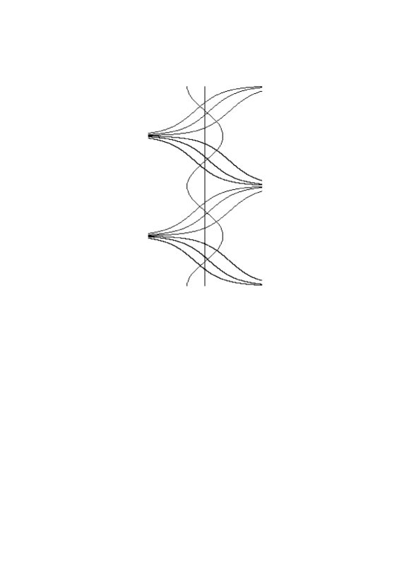
Figure 1: The trajectories crossing the line $\{x_{1}=0\}$ and the equipotential $\{u=0\}$

Consider the line $\{x_{1}=0\}$ as the hyperplane $H$. Then, we have $\tau_{H}(x)=-\,x_{1}$. Moreover, using successively the explicit formula (2.27) and the semigroup property (2.35), we get that

$$X\big{(}\!-\!X_{1}(t,x),X(t,x)\big{)}=X\big{(}\!-t-x_{1},X(t,x)\big{)}=X(-\,x_{1},x),\quad\mbox{for any }t\in\mathbb{R}.$$ (2.28)

Hence, the function $v$ defined by $v(x):=X_{2}(-\,x_{1},x)$ satisfies

$$v\big{(}X(t,x)\big{)}=X_{2}\big{(}\!-\!X_{1}(t,x),X(t,x)\big{)}=X_{2}(-\,x_{1},x)=v(x),\quad\mbox{for any }t\in\mathbb{R}.$$ (2.29)

The function $v$ is thus a first integral of system (2.25). It follows that

$${d\over dt}\left[v\big{(}X(t,x)\big{)}\right]=0=\nabla v\big{(}X(t,x)\big{)}\cdot{dX\over dt}(t,x)=\nabla v\big{(}X(t,x)\big{)}\cdot\nabla u\big{(}X(t,x)\big{)},$$ (2.30)

which, taking $t=0$, implies that $\nabla u\cdot\nabla v=0$ in $\mathbb{R}^{2}$. Moreover, putting $t=-\,x_{1}$ in (2.27), we get that for any $n\in\mathbb{Z}$,

$$v(x)=\left\{\begin{array}[]{cl}n+{1\over\pi}\arctan\big{(}e^{-4\pi^{2}x_{1}}\tan(\pi x_{2})\big{)}&\mbox{if }x_{2}\in\left(n-{1\over 2},n+{1\over 2}\right)\\ \vskip 6.0pt plus 2.0pt minus 2.0pt\cr n+{1\over 2}&\mbox{if }x_{2}=n+{1\over 2}.\end{array}\right.$$ (2.31)

Therefore, by (2.13) $\nabla u$ is an isotropically realizable electric field in the whole space $\mathbb{R}^{2}$, with the smooth conductivity

$$\sigma:={|\nabla v|\over|\nabla u|}=\left\{\begin{array}[]{cl}\displaystyle{1+\tan^{2}(\pi x_{2})\over e^{4\pi^{2}x_{1}}+e^{-4\pi^{2}x_{1}}\tan^{2}(\pi x_{2})}&\mbox{if }x_{2}\notin{1\over 2}+\mathbb{Z}\\ \vskip 6.0pt plus 2.0pt minus 2.0pt\cr\displaystyle e^{4\pi^{2}x_{1}}&\mbox{if }x_{2}\in{1\over 2}+\mathbb{Z}.\end{array}\right.$$ (2.32)

It may be checked by a direct calculation that $\sigma\nabla u$ is divergence free in $\mathbb{R}^{2}$.

Proof of Theorem 2.10. Let $(\tau_{1},\dots,\tau_{d-1})$ be an orthonormal basis of the hyperplane $H$. Define for each $k\in\{1,\dots,d-1\}$, the function $v_{k}$ by

$$v_{k}(x):=z_{H}(x)\cdot\tau_{k}=X\big{(}\tau_{H}(x),x\big{)}\cdot\tau_{k},\quad\mbox{for }x\in\mathbb{R}^{d}.$$ (2.33)

We shall prove that the functions $v_{k}$ satisfy the properties of the proof of Theorem 2.2. $i)$.

First, due the transversality of each trajectory across $H$, we have for any $x\in\mathbb{R}^{d}$,

$$\left.{\partial\over\partial t}\big{(}X(t,x)\cdot\nu\big{)}\right|_{t=\tau_{H}(x)}=\nabla u\big{(}z_{H}(x)\big{)}\cdot\nu\neq 0.$$ (2.34)

Hence, the implicit functions theorem combined with the $C^{1}$-regularity of $(t,x)\mapsto X(t,x)$ (see, e.g., [4], Theorem $\rm T^{\prime}_{r}$ p. 222) implies that $x\mapsto\tau_{H}(x)$ defines a function in $C^{1}(\mathbb{R}^{d})$. Therefore, the functions $v_{k}$ defined by (2.33) belong to $C^{1}(\mathbb{R})$.

Second, since the trajectories satisfy the identity

$$X\big{(}s,X(t,x)\big{)}=X(s+t,x)\quad\forall\,s,t\in\mathbb{R},\ \forall\,x\in\mathbb{R}^{d},$$ (2.35)

we get that $X\big{(}\tau_{H}(x)-t,X(t,x)\big{)}=X\big{(}\tau_{H}(x),x\big{)}$, and thus

$$\tau_{H}\big{(}X(t,x)\big{)}=\tau_{H}(x)-t.$$ (2.36)

It follows that for any $k\in\{1,\dots,d-1\}$,

$$v_{k}\big{(}X(t,x)\big{)}=X\big{(}\tau_{H}(x)-t,X(t,x)\big{)}\cdot\tau_{k}=X\big{(}\tau_{H}(x),x)\big{)}\cdot\tau_{k},\quad\mbox{for any }t\in\mathbb{R}.$$ (2.37)

Therefore, each function $v_{k}$ is a first integral of the dynamical system (2.25).

Third, consider for some $x_{0}\in\Omega$, a vector $(\lambda_{1},\dots,\lambda_{d-1}\big{)}\in\mathbb{R}^{d-1}$ such that

$$\sum_{k=1}^{d-1}\lambda_{k}\nabla v_{k}(x_{0})=0,$$ (2.38)

and define the function

$$v_{0}:=\sum_{k=1}^{d-1}\lambda_{k}\,v_{k}=z_{H}\cdot\tau_{0},\quad\mbox{where}\quad\tau_{0}:=\sum_{k=1}^{d-1}\lambda_{k}\,\tau_{k}.$$ (2.39)

By the chain rule we have

$$\begin{array}[]{ll}Dz_{H}(x)&\displaystyle=\nabla\tau_{H}(x)\otimes{\partial X\over\partial t}\big{(}\tau_{H}(x),x\big{)}+D_{x}X\big{(}\tau_{H}(x),x\big{)}\\ \vskip 6.0pt plus 2.0pt minus 2.0pt\cr&\displaystyle=\nabla\tau_{H}(x)\otimes\nabla u\big{(}z_{H}(x)\big{)}+D_{x}X\big{(}\tau_{H}(x),x\big{)}.\end{array}$$ (2.40)

This combined with the equality (recall that $z_{H}(x)\in H$)

$$0=\left.\nabla\big{(}z_{H}(x)\cdot\nu\big{)}\right|_{x=x_{0}}=Dz_{H}(x_{0})\,\nu,$$ (2.41)

implies that

$$\nabla\tau_{H}(x_{0})={-1\over\nabla u\big{(}z_{H}(x_{0})\big{)}\cdot\nu}\,D_{x}X\big{(}\tau_{H}(x_{0}),x_{0}\big{)}\,\nu.$$ (2.42)

Hence, by the equalities (2.38), (2.39) and again using (2.40) together with (2.42), we get that

$$0=\nabla v_{0}(x_{0})=Dz_{H}(x_{0})\,\tau_{0}=D_{x}X\big{(}\tau_{H}(x_{0}),x_{0}\big{)}\left(\tau_{0}-{\nabla u\big{(}z_{H}(x_{0})\big{)}\cdot\tau_{0}\over\nabla u\big{(}z_{H}(x_{0})\big{)}\cdot\nu}\,\nu\right).$$ (2.43)

However, by Lemma 2.12 below, the matrix $D_{x}X\big{(}\tau_{H}(x_{0}),x_{0}\big{)}$ is invertible. This combined with (2.43) yields that $\tau_{0}$ is proportional to $\nu$. Hence, $\tau_{0}=0$ and $(\nabla v_{1},\dots,\nabla v_{d-1})$ has rank $(d-1)$ everywhere in $\mathbb{R}^{d}$. Therefore, the continuous positive conductivity defined by (2.11) shows that $\nabla u$ is isotropically realizable in the whole space $\mathbb{R}^{d}$. $\Box$

Lemma 2.12.

The derivative $D_{x}X$ of the dynamical system (2.25) is invertible in $\mathbb{R}\times\mathbb{R}^{d}$.

Proof.

By the chain rule the matrix field $D_{x}X$ satisfies the variational equation

$$\left\{\begin{array}[]{rl}\displaystyle{d\over dt}D_{x}X(t,x)&=D_{x}X(t,x)\,\nabla^{2}u\big{(}X(t,x)\big{)}\\ \vskip 6.0pt plus 2.0pt minus 2.0pt\cr D_{x}X(0,x)&=I_{d},\end{array}\right.\quad\mbox{for }t\in\mathbb{R},\ x\in\mathbb{R}^{d},$$ (2.44)

where $\nabla^{2}u$ denotes the Hessian matrix of $u$ and $I_{d}$ is the unit matrix of $\mathbb{R}^{d\times d}$. Moreover, due to the multi-linearity of the determinant $\det\left(D_{x}X\right)$ satisfies Liouville’s formula

$$\left\{\begin{array}[]{rl}\displaystyle{d\over dt}\det\left(D_{x}X\right)(t,x)&={\rm tr}\left[\nabla^{2}u\big{(}X(t,x)\big{)}\right]\det\left(D_{x}X\right)(t,x)\\ \vskip 6.0pt plus 2.0pt minus 2.0pt\cr\det\left(D_{x}X\right)(0,x)&=1,\end{array}\right.\quad\mbox{for }t\in\mathbb{R},\ x\in\mathbb{R}^{d},$$ (2.45)

where tr denotes the trace. It follows that

$$\det\left(D_{x}X\right)(t,x)=\exp\left(\int_{0}^{t}{\rm tr}\left[\nabla^{2}u\big{(}X(s,x)\big{)}\right]ds\right)>0\quad\mbox{for any }(t,x)\in\mathbb{R}\times\mathbb{R}^{d},$$ (2.46)

which shows that $D_{x}X(t,x)$ is invertible. ∎

Remark 2.13.

The hyperplane assumption of Theorem 2.10 does not hold in general. Indeed, we have the following heuristic argument:

Let $H$ be a line of $\mathbb{R}^{2}$, and let $\Sigma$ be a smooth curve of $\mathbb{R}^{2}$ having an $S$-shape across $H$. Consider a smooth periodic isotropic conductivity $\sigma$ which is very small in the neighborhood of $\Sigma$. Let $u$ be a smooth potential solution of $\mbox{\rm div}\left(\sigma\nabla u\right)=0$ in $\mathbb{R}^{2}$ satisfying (2.2), (2.3), and let $v$ be the associated stream function satisfying $\sigma\nabla u=R_{\perp}\nabla v$ in $\mathbb{R}^{2}$. The potential $v$ is solution of $\mbox{\rm div}\left(\sigma^{-1}\nabla v\right)=0$ in $\mathbb{R}^{2}$. Then, since $\sigma^{-1}$ is very large in the neighborhood of $\Sigma$, the curve $\Sigma$ is close to an equipotential of $v$ and thus close to a current line of $u$. Therefore, some trajectory of (2.25) has an $S$-shape across $H$. This makes impossible the regularity of the time $\tau_{H}$ which is actually a multi-valued function.

2.2.2 Isotropic realizability in the whole space

Replacing a hyperplane by an equipotential (see figure 1 above) we have the more general result:

Theorem 2.14.

Let $u$ be a function in $C^{3}(\mathbb{R}^{d})$ such that $\nabla u$ satisfies (2.2) and (2.3). Then, the gradient field $\nabla u$ is an isotropically realizable electric field in $\mathbb{R}^{d}$.

Proof.

On the one hand, for a fixed $x\in\mathbb{R}^{d}$, define the function $f:\mathbb{R}\to\mathbb{R}$ by $f(t):=u\big{(}X(t,x)\big{)}$, for $t\in\mathbb{R}$. The function $f$ is in $C^{3}(\mathbb{R})$, and

$$f^{\prime}(t)={dX\over dt}(t,x)\cdot\nabla u\big{(}X(t,x)\big{)}=\left|\nabla u\big{(}X(t,x)\big{)}\right|^{2},\quad\forall\,t\in\mathbb{R}.$$ (2.47)

Since $\nabla u$ is periodic, continuous and does not vanish in $\mathbb{R}^{d}$, there exists a constant $m>0$ such that $f^{\prime}\geq m$ in $\mathbb{R}$. It follows that

$${f(t)-f(0)\over t}\geq m,\quad\forall\,t\in\mathbb{R}\setminus\{0\},$$ (2.48)

which implies that

$$\lim_{t\to\infty}f(t)=\infty\quad\mbox{and}\quad\lim_{t\to-\infty}f(t)=-\infty.$$ (2.49)

This combined with the monotonicity and continuity of $f$ thus shows that there exists a unique $\tau(x)\in\mathbb{R}$ such that

$$u\big{(}X(\tau(x),x)\big{)}=0.$$ (2.50)

On the other hand, similar to the hyperplane case, we have that for any $x\in\mathbb{R}^{d}$,

$$\left.{\partial\over\partial t}\left[u\big{(}X(t,x)\big{)}\right]\right|_{t=\tau(x)}=\left|\nabla u\big{(}X(\tau(x),x)\big{)}\right|^{2}>0.$$ (2.51)

Hence, from the implicit functions theorem combined with the $C^{2}$-regularity of $(t,x)\mapsto u\big{(}X(t,x)\big{)}$ we deduce that $x\mapsto\tau(x)$ is a function in $C^{2}(\mathbb{R}^{d})$.

Now define the function $w$ in $\mathbb{R}^{d}$ by

$$w(x):=\int_{0}^{\tau(x)}\Delta u\big{(}X(s,x)\big{)}\,ds,\quad\mbox{for }x\in\mathbb{R}^{d},$$ (2.52)

which belongs to $C^{1}(\mathbb{R}^{d})$ since $u\in C^{3}(\mathbb{R}^{d})$. Then, using (2.35), (2.36) and the change of variable $r:=s+t$, we have for any $(t,x)\in\mathbb{R}\times\mathbb{R}^{d}$,

$$w\big{(}X(t,x)\big{)}=\int_{0}^{\tau(x)-t}\Delta u\big{(}X(s+t,x)\big{)}\,ds=\int_{t}^{\tau(x)}\Delta u\big{(}X(r,x)\big{)}\,dr,$$ (2.53)

which implies that

$${\partial\over\partial t}\left[w\big{(}X(t,x)\big{)}\right]=\nabla w\big{(}X(t,x)\big{)}\cdot\nabla u\big{(}X(t,x)\big{)}=-\Delta u\big{(}X(t,x)\big{)}.$$ (2.54)

Finally, define the conductivity $\sigma$ by

$$\sigma(x):=e^{w(x)}=\exp\left(\int_{0}^{\tau(x)}\Delta u\big{(}X(s,x)\big{)}\,ds\right),\quad\mbox{for }x\in\mathbb{R}^{2},$$ (2.55)

which belongs to $C^{1}(\mathbb{R}^{d})$. Applying (2.54) with $t=0$, we obtain that

$$\mbox{\rm div}\left(\sigma\nabla u\right)=e^{w}\left(\nabla w\cdot\nabla u+\Delta u\right)=0\quad\mbox{in }\mathbb{R}^{d},$$ (2.56)

which concludes the proof. ∎

Remark 2.15.

In the proof of Theorem 2.14 the condition that $\nabla u$ is non-zero everywhere is essential to obtain both:

- the uniqueness of the time $\tau(x)$ for each trajectory to reach the equipotential $\{u=0\}$,

- the regularity of the function $x\mapsto\tau(x)$.

2.2.3 Isotropic realizability in the torus

We have the following characterization of the isotropic realizability in the torus:

Theorem 2.16.

Let $u$ be a function in $C^{3}(\mathbb{R}^{d})$ such that $\nabla u$ satisfies (2.2) and (2.3).

Then, the gradient field $\nabla u$ is isotropically realizable with a positive conductivity $\sigma\in L^{\infty}_{\sharp}(Y)$, with $\sigma^{-1}\in L^{\infty}_{\sharp}(Y)$, if there exists a constant $C>0$ such that

$$\forall\,x\in\mathbb{R}^{d},\quad\left|\,\int_{0}^{\tau(x)}\Delta u\big{(}X(t,x)\big{)}\,dt\,\right|\leq C,$$ (2.57)

where $X(t,x)$ is defined by (2.25) and $\tau(x)$ by (2.50).

Conversely, if $\nabla u$ is isotropically realizable with a positive conductivity $\sigma\in C^{1}_{\sharp}(Y)$, then the boundedness (2.57) holds.

Example 2.17.

For the function $u$ of Example 2.11 and for $x=(x_{1},0)$, we have by (2.57) and (2.27),

$$\sigma_{0}(x)=\exp\left(4\pi^{2}\int_{0}^{\tau(x)}\cos\big{(}2\pi X_{2}(s,x)\big{)}\,ds\right)=\exp\left(4\pi^{2}\,\tau(x)\right),$$

and by (2.50),

$$X_{1}\big{(}\tau(x),x\big{)}=\tau(x)+x_{1}=\cos\big{(}2\pi X_{2}(\tau(x),x)\big{)}=1.$$

Therefore, we get that $\sigma_{0}(x_{1},0)=\exp\big{(}4\pi^{2}\,(1-x_{1})\big{)}$, which contradicts the boundedness (2.57). This is consistent with the negative conclusion of Example 2.6.

Proof of Theorem 2.16.

Sufficient condition: Without loss of generality we may assume that the period is $Y=[0,1]^{d}$. Define the function $\sigma_{0}$ by

$$\sigma_{0}(x):=\exp\left(\int_{0}^{\tau(x)}\Delta u\big{(}X(t,x)\big{)}\,dt\right),\quad\mbox{for }x\in\mathbb{R}^{d},$$ (2.58)

and consider for any integer $n\geq 1$, the conductivity $\sigma_{n}$ defined by the average over the $(2n+1)^{d}$ integer vectors of $[-n,n]^{d}$:

$$\sigma_{n}(x):={1\over(2n+1)^{d}}\sum_{k\in\mathbb{Z}^{d}\cap[-n,n]^{d}}\sigma_{0}(x+k),\quad\mbox{for }x\in\mathbb{R}^{d}.$$ (2.59)

On the one hand, by (2.57) $\sigma_{n}$ is bounded in $L^{\infty}(\mathbb{R}^{d})$. Hence, there is a subsequence of $n$, still denoted by $n$, such that $\sigma_{n}$ converges weakly-$*$ to some function $\sigma$ in $L^{\infty}(\mathbb{R}^{d})$. Moreover, we have for any $x\in\mathbb{R}^{d}$ and any $k\in\mathbb{Z}^{d}$ (denoting $\displaystyle|k|_{\infty}:=\max_{1\leq i\leq d}|k_{i}|$),

$$\begin{array}[]{ll}\left|\,(2n+1)^{d}\,\sigma_{n}(x+k)-(2n+1)^{d}\,\sigma_{n}(x)\,\right|&\displaystyle=\Big{|}\,\sum_{|j-k|_{\infty}\leq n}\sigma_{0}(x+j)-\sum_{|j|_{\infty}\leq n}\sigma_{0}(x+j)\,\Big{|}\\ \vskip 6.0pt plus 2.0pt minus 2.0pt\cr&\displaystyle\leq\sum_{\begin{array}[]{c}{}^{|j-k|_{\infty}\leq n}\\[-4.26773pt] {}^{|j|_{\infty}>n}\end{array}}\kern-5.69046pt\sigma_{0}(x+j)+\kern-5.69046pt\sum_{\begin{array}[]{c}{}^{|j-k|_{\infty}>n}\\[-4.26773pt] {}^{|j|_{\infty}\leq n}\end{array}}\kern-5.69046pt\sigma_{0}(x+j)\\ &\leq C\,n^{d-1},\end{array}$$ (2.60)

where $C$ is a constant independent of $n$ and $x$. This implies that $\sigma(\cdot+k)=\sigma(\cdot)$ a.e. in $\mathbb{R}^{d}$, for any $k\in\mathbb{Z}^{d}$. The function $\sigma$ is thus $Y$-periodic and belongs to $L^{\infty}_{\sharp}(Y)$. Moreover, since by virtue of (2.57) and (2.58) $\sigma_{0}$ is bounded from below by $e^{-C}$, so is $\sigma_{n}$ and its limit $\sigma$. Therefore, $\sigma^{-1}$ also belongs to $L^{\infty}_{\sharp}(Y)$.

On the other hand, by virtue of Theorem 2.14 the gradient field $\nabla u$ is realizable in $\mathbb{R}^{d}$ with the conductivity $\sigma_{0}$. This combined with the $Y$-periodicity of $\nabla u$ yields $\mbox{\rm div}\left(\sigma_{n}\nabla u\right)=0$ in $\mathbb{R}^{d}$. Hence, using the weak-$*$ convergence of $\sigma_{n}$ in $L^{\infty}(\mathbb{R}^{d})$ we get that for any $\varphi\in C^{\infty}_{c}(\mathbb{R}^{d})$, $\nabla u\cdot\nabla\varphi\in L^{1}(\mathbb{R}^{d})$ and

$$0=\lim_{n\to\infty}\int_{\mathbb{R}^{d}}\sigma_{n}\nabla u\cdot\nabla\varphi\,dx=\int_{\mathbb{R}^{d}}\sigma\nabla u\cdot\nabla\varphi\,dx.$$ (2.61)

Therefore, we obtain that $\mbox{\rm div}\left(\sigma\nabla u\right)=0$ in $\mathscr{D}^{\prime}(\mathbb{R}^{d})$, so that $\nabla u$ is isotropically realizable with the $Y$-periodic bounded conductivity $\sigma$.

Necessary condition: Let $\sigma$ be a positive function in $C^{1}_{\sharp}(Y)$ such that $\mbox{\rm div}\left(\sigma\nabla u\right)=0$ in $\mathbb{R}^{d}$. Then, the function $w:=\ln\sigma$ also belongs to $C^{1}_{\sharp}(Y)$, and solves the equation $\nabla w\cdot\nabla u+\Delta u=0$ in $\mathbb{R}^{d}$. Therefore, using (2.25) we obtain that for any $x\in\mathbb{R}^{d}$,

$$\begin{array}[]{ll}\displaystyle\int_{0}^{\tau(x)}\Delta u\big{(}X(t,x)\big{)}\,dt&\displaystyle=-\int_{0}^{\tau(x)}\nabla w\big{(}X(t,x)\big{)}\cdot\nabla u\big{(}X(t,x)\big{)}\,dt\\ \vskip 6.0pt plus 2.0pt minus 2.0pt\cr&\displaystyle=-\int_{0}^{\tau(x)}\nabla w\big{(}X(t,x)\big{)}\cdot{dX\over dt}(t,x)\,dt\\ \vskip 6.0pt plus 2.0pt minus 2.0pt\cr&=w\big{(}X(0,x)\big{)}-w\big{(}X(\tau(x),x)\big{)}=w(x)-w\big{(}X(\tau(x),x)\big{)},\end{array}$$ (2.62)

which implies (2.57) due to the boundedness of $w$ in $\mathbb{R}^{d}$. $\Box$

Remark 2.18.

If we also assume that $\sigma_{0}$ of (2.57) is uniformly continuous in $\mathbb{R}^{d}$, then the previous proof combined with Ascoli’s theorem implies that the conductivity $\sigma$ is continuous. Indeed, the sequence $\sigma_{n}$ defined by (2.59) is then equi-continuous.

3 The matrix field case

Definition 3.1.

Let $\Omega$ be an (bounded or not) open set of $\mathbb{R}^{d}$, $d\geq 2$, and let $U=(u_{1},\dots,u_{d})$ be a function in $H^{1}(\Omega)^{d}$. The matrix-valued field $DU$ is said to be a realizable matrix-valued electric field in $\Omega$ if there exists a symmetric positive definite matrix-valued $\sigma\in L^{\infty}_{\rm loc}(\Omega)^{d\times d}$ such that

$$\mbox{\rm Div}\left(\sigma DU\right)=0\quad\mbox{in }\mathscr{D}^{\prime}(\Omega).$$ (3.1)

3.1 The periodic framework

Theorem 3.2.

Let $Y$ be a closed parallelepiped of $\mathbb{R}^{d}$, $d\geq 2$. Consider a function $U\in C^{1}(\mathbb{R}^{d})^{d}$ such that

$$DU\mbox{ is $Y$-periodic}\quad\mbox{and}\quad\det\big{(}\langle DU\rangle\big{)}\neq 0.$$ (3.2)

• Assume that

  $$\det\big{(}\langle DU\rangle DU\big{)}>0\quad\mbox{everywhere in }\mathbb{R}^{d}.$$ (3.3)

  Then, $DU$ is a realizable electric matrix field in $\mathbb{R}^{d}$ associated with a continuous conductivity.

• Assume that $d=2$, and that $DU$ is a realizable electric matrix field in $\mathbb{R}^{2}$, satisfying (3.2) and associated with a smooth conductivity in $\mathbb{R}^{2}$. Then, condition (3.3) holds true.

• In dimension $d=3$, there exists a smooth matrix field $DU$ satisfying (3.2) and associated with a smooth periodic conductivity, such that $\det\left(DU\right)$ takes positive and negative values in $\mathbb{R}^{3}$.

Remark 3.3.

Similarly to Remark 2.8 the assertions $i)$ and $ii)$ of Theorem 3.2 still hold under the less regular assumptions that

$$DU\in L^{2}_{\sharp}(Y)^{d\times d}\quad\mbox{and}\quad\det\big{(}\langle DU\rangle DU\big{)}>0\;\;\mbox{a.e. in }\mathbb{R}^{d}.$$ (3.4)

Then, the $Y$-periodic conductivity $\sigma$ defined by the formula (3.5) below is only defined a.e. in $\mathbb{R}^{d}$, and is not necessarily uniformly bounded from below or above in the cell period $Y$. However, $\sigma DU$ remains divergence free in the sense of distributions on $\mathbb{R}^{d}$.

Proof of Theorem 3.2.

$i)$ Let $U\in C^{1}(\mathbb{R}^{d})^{d}$ be a vector-valued function satisfying (3.2). Then, we can define the matrix-valued function $\sigma$ by

$$\sigma:=\det\big{(}\langle DU\rangle DU\big{)}\,(DU^{-1})^{T}DU^{-1}=\det\big{(}\langle DU\rangle\big{)}\,{\rm Cof}\left(DU\right)DU^{-1},$$ (3.5)

where ${\rm Cof}$ denotes the Cofactors matrix. It is clear that $\sigma$ is a $Y$-periodic continuous symmetric positive definite matrix-valued function. Moreover, Piola’s identity (see, e.g., [11], Theorem 3.2) implies that

$$\mbox{\rm Div}\,\big{(}{\rm Cof}\left(DU\right)\big{)}=0\quad\mbox{in }\mathscr{D}^{\prime}(\mathbb{R}^{d}).$$ (3.6)

Hence, $\sigma DU$ is Divergence free in $\mathbb{R}^{d}$. Therefore, $DU$ is a realizable electric matrix field associated with the continuous conductivity $\sigma$.

$ii)$ Let $DU$ be an electric matrix field satisfying condition (3.2) and associated with a smooth conductivity in $\mathbb{R}^{2}$. By the regularity results for second-order elliptic pde’s the function $U$ is smooth in $\mathbb{R}^{2}$. Moreover, due to [1] (Theorem 1) we have $\det\big{(}\langle DU\rangle DU\big{)}>0$ a.e. in $\mathbb{R}^{2}$. Therefore, as in the proof of Theorem 2.7 we conclude that (3.3) holds.

$iii)$ This is an immediate consequence of the counter-example of [8] combined with the regularization argument used in the proof of Theorem 2.2 $iii)$. $\Box$

Remark 3.4.

The conductivity $\sigma$ defined by (3.5) can be derived by applying the coordinate change $x^{\prime}=U^{-1}(x)$ to the homogeneous conductivity $\big{|}\det\langle DU\rangle\big{|}\,I_{d}$.

In fact there are many ways to derive a conductivity $\sigma$ associated with a matrix field $DU$ the determinant of which has a constant sign. Following [14] (Remark p. 155) such a conductivity can be expressed by $\sigma=JDU^{-1}$, where $J$ is a Divergence free matrix-valued function. From this perspective we have the following extension of part $i)$ of Theorem 3.2:

Proposition 3.5.

Let $U$ be a function in $C^{1}(\mathbb{R}^{d})^{d}$ satisfying (3.2) and (3.3). Consider a convex function $\varphi$ in $C^{2}(\mathbb{R}^{d})$ whose Hessian matrix $\nabla^{2}\varphi$ is positive definite everywhere in $\mathbb{R}^{d}$. Then, $Du$ is a realizable electric matrix field with the conductivity

$$\sigma:=JDU^{-1}\quad\mbox{where}\quad J:=\det\big{(}\langle DU\rangle\big{)}\,{\rm Cof}\,\big{(}D(\nabla\varphi\circ U)\big{)}.$$ (3.7)

Proof.

On the one hand, the matrix-valued function $J$ of (3.7) is clearly Divergence free due to Piola’s identity. On the other hand, we have

$${\rm Cof}\,\big{(}D(\nabla\varphi\circ U)\big{)}={\rm Cof}\,\big{(}DU\,\nabla^{2}\varphi\circ U\big{)}={\rm Cof}\left(DU\right){\rm Cof}\left(\nabla^{2}\varphi\circ U\right),$$ (3.8)

so that the matrix-valued $\sigma$ defined by (3.7) satisfies

$$\sigma=\det\big{(}\langle DU\rangle DU\big{)}\,(DU^{-1})^{T}\,{\rm Cof}\left(\nabla^{2}\varphi\circ U\right)DU^{-1}.$$ (3.9)

Since $\nabla^{2}\varphi$ is symmetric positive definite, so is its Cofactors matrix. Therefore, $\sigma$ is an admissible continuous conductivity such that $\sigma DU$ is Divergence free in $\mathbb{R}^{d}$. ∎

3.2 The laminate case

		${}_{\textstyle\sigma^{1}_{1,2}}$			${}_{\textstyle\sigma^{1}_{1,2}}$
		${}_{\textstyle\sigma^{2}_{1,2}}$			${}_{\textstyle\sigma^{2}_{1,2}}$
${}_{\textstyle\sigma^{1}_{1,1}}$	${}_{\textstyle\sigma^{2}_{1,1}}$	${}_{\textstyle\sigma^{1}_{1,2}}$	${}_{\textstyle\sigma^{1}_{1,1}}$	${}_{\textstyle\sigma^{2}_{1,1}}$	${}_{\textstyle\sigma^{1}_{1,2}}$
		${}_{\textstyle\sigma^{2}_{1,2}}$			${}_{\textstyle\sigma^{2}_{1,2}}$
		${}_{\textstyle\sigma^{1}_{1,2}}$			${}_{\textstyle\sigma^{1}_{1,2}}$

Figure 2: A rank-two laminate with directions $\xi_{1}=e_{1}$ and $\xi_{1,2}=e_{2}$

Definition 3.6.

Let $d,n$ be two positive integers. A rank-$n$ laminate in $\mathbb{R}^{d}$ is a multiscale microstructure defined at $n$ ordered scales $\varepsilon_{n}\ll\cdots\ll\varepsilon_{1}$ depending on a small positive parameter $\varepsilon\to 0$, and in multiple directions in $\mathbb{R}^{d}\setminus\{0\}$, by the following process (see figure 2):

• At the smallest scale $\varepsilon_{n}$, there is a set of $m_{n}$ rank-one laminates, the $i^{\rm th}$ one of which is composed, for $i=1,\dots,m_{n}$, of an $\varepsilon_{n}$-periodic repetition in the direction $\xi_{i,n}$ of homogeneous layers with constant positive definite conductivity matrices $\sigma^{h}_{i,n}$, $h\in I_{i,n}$.

• At the scale $\varepsilon_{k}$, there is a set of $m_{k}$ laminates, the $i^{\rm th}$ one of which is composed, for $i=1,\dots,m_{k}$, of an $\varepsilon_{k}$-periodic repetition in the direction $\xi_{i,k}\in\mathbb{R}^{d}\setminus\{0\}$ of homogeneous layers and$/$or a selection of the $m_{k+1}$ laminates which are obtained at stage $(k+1)$ with conductivity matrices $\sigma^{h}_{i,j}$, for $j=k+1,\dots,n$, $h\in I_{i,j}$.

• At the scale $\varepsilon_{1}$, there is a single laminate ($m_{1}=1$) which is composed of an $\varepsilon_{1}$-periodic repetition in the direction $\xi_{1}\in\mathbb{R}^{d}\setminus\{0\}$ of homogeneous layers and$/$or a selection of the $m_{2}$ laminates which are obtained at the scale $\varepsilon_{2}$ with conductivity matrices $\sigma^{h}_{i,j}$, for $j=2,\dots,n$, $h\in I_{i,j}$.

The laminate conductivity at stage $k=1,\dots,n$, is denoted by $L^{\varepsilon}_{k}(\hat{\sigma})$, where $\hat{\sigma}$ is the whole set of the constant laminate conductivities.

Due to the results of [13, 7] there exists a set $\hat{P}$ of constant matrices in $\mathbb{R}^{d\times d}$, such that the laminate $P_{\varepsilon}:=L^{\varepsilon}_{n}(\hat{P})$ is a corrector (or a matrix electric field) associated with the conductivity $\sigma_{\varepsilon}:=L^{\varepsilon}_{n}(\hat{\sigma})$ in the sense of Murat-Tartar [15], i.e.

$$\left\{\begin{array}[]{rl}P_{\varepsilon}\rightharpoonup I_{d}&\mbox{weakly in }L^{2}_{\rm loc}(\mathbb{R}^{d})^{d\times d},\\ \vskip 6.0pt plus 2.0pt minus 2.0pt\cr\mbox{\rm Curl}\left(P_{\varepsilon}\right)\to 0&\mbox{strongly in }H^{-1}_{\rm loc}(\mathbb{R}^{d})^{d\times d\times d},\\ \vskip 6.0pt plus 2.0pt minus 2.0pt\cr\mbox{\rm Div}\left(\sigma_{\varepsilon}P_{\varepsilon}\right)&\mbox{is compact in }H^{-1}_{\rm loc}(\mathbb{R}^{d})^{d}.\end{array}\right.$$ (3.10)

The weak limit of $\sigma_{\varepsilon}P_{\varepsilon}$ in $L^{2}_{\rm loc}(\mathbb{R}^{d})^{d\times d}$ is then the homogenized limit of the laminate. The three conditions of (3.10) satisfied by $P_{\varepsilon}$ extend to the laminate case the three respective conditions

$$\left\{\begin{array}[]{l}\langle DU\rangle=I_{d},\\ \vskip 6.0pt plus 2.0pt minus 2.0pt\cr\mbox{\rm Curl}\left(DU\right)=0,\\ \vskip 6.0pt plus 2.0pt minus 2.0pt\cr\mbox{\rm Div}\left(\sigma DU\right)=0,\end{array}\right.$$ (3.11)

satisfied by any electric matrix field $DU$ in the periodic case.

The equivalent of Theorem 3.2 for a laminate is the following:

Theorem 3.7.

Let $n,d$ be two positive integers. Consider a rank-$n$ laminate $L^{\varepsilon}_{n}(\hat{P})$ built from a finite set $\hat{P}$ of $\mathbb{R}^{d\times d}$ (according to Definition 3.6) which satisfies the two first conditions of (3.10). Then, a necessary and sufficient condition for $L^{\varepsilon}_{n}(\hat{P})$ to be a realizable laminate electric field, i.e. to satisfy the third condition of (3.10) for some rank-$n$ laminate conductivity $L^{\varepsilon}_{n}(\hat{\sigma})$, is that $\det\big{(}L^{\varepsilon}_{n}(\hat{P})\big{)}>0$ a.e. in $\mathbb{R}^{d}$, or equivalently that the determinant of each matrix in $\hat{P}$ is positive.

Proof of Theorem 3.7. The fact that the determinant positivity condition is necessary was established in [8], Theorem 3.3 (see also [9], Theorem 2.13, for an alternative approach).

Conversely, consider a rank-$n$ laminate field $P_{\varepsilon}=L^{\varepsilon}_{n}(\hat{P})$ satisfying the two first convergence of (3.10) and $\det\left(P_{\varepsilon}\right)>0$ a.e. in $\mathbb{R}^{d}$, or equivalently $\det\left(P\right)>0$ for any $P\in\hat{P}$. Similarly to (3.5) consider the rank-$n$ laminate conductivity defined by

$$\sigma_{\varepsilon}:=\det\big{(}P_{\varepsilon}\big{)}\,(P_{\varepsilon}^{-1})^{T}(P_{\varepsilon})^{-1}=L^{\varepsilon}_{n}(\hat{\sigma}),\quad\mbox{where}\quad\hat{\sigma}:=\big{\{}\det\big{(}P\big{)}\,(P^{-1})^{T}P^{-1}:P\in\hat{P}\big{\}}.$$ (3.12)

Then, the third condition of (3.10) is equivalent to the condition

$$\mbox{\rm Div}\,\big{(}{\rm Cof}\left(P_{\varepsilon}\right)\big{)}\quad\mbox{is compact in }H^{-1}_{\rm loc}(\mathbb{R}^{d})^{d}.$$ (3.13)

Contrary to the periodic case ${\rm Cof}\left(P_{\varepsilon}\right)$ is not divergence free in the sense of distributions. However, following the homogenization procedure for laminates of [7], and using the quasi-affinity of the Cofactors for gradients (see, e.g., [11]), condition (3.13) holds if any matrices $P,Q$ of two neighboring layers in a direction $\xi$ of the laminate satisfy the jump condition for the divergence

$$\big{(}{\rm Cof}\left(P\right)-{\rm Cof}\left(Q\right)\big{)}^{T}\xi=0.$$ (3.14)

More precisely, at a given scale $\varepsilon_{k}$ of the laminate the matrix $P$, or $Q$, is:

• either a matrix in $\hat{P}$,

• or the average of rank-one laminates obtained at the smallest scales $\varepsilon_{k+1},\dots,\varepsilon_{n}$.

In the first case the matrix $P$ is the constant value of the field in a homogeneous layer of the rank-$n$ laminate. In the second case the average of the Cofactors of the matrices involving in these rank-one laminations is equal to the Cofactors matrix of the average, that is ${\rm Cof}\left(P\right)$, by virtue of the quasi-affinity of the Cofactors applied iteratively to the rank-one connected matrices in each rank-one laminate.

Therefore, it remains to prove equality (3.14) for any matrices $P,Q$ with positive determinant satisfying the condition which controls the jumps in the second convergence of (3.10), namely

$$P-Q=\xi\otimes\eta\quad\mbox{for some }\eta\in\mathbb{R}^{d}.$$ (3.15)

By (3.15) and by the multiplicativity of the Cofactors matrix we have

$$\begin{array}[]{ll}\big{(}{\rm Cof}\left(P\right)-{\rm Cof}\left(Q\right)\big{)}^{T}&={\rm Cof}\left(Q\right)^{T}\left[{\rm Cof}\left(I_{d}+\left(\xi\otimes\eta\right)Q^{-1}\right)^{T}-I_{d}\right]\\ \vskip 6.0pt plus 2.0pt minus 2.0pt\cr&={\rm Cof}\left(Q\right)^{T}\left[{\rm Cof}\left(I_{d}+\xi\otimes\lambda\right)^{T}-I_{d}\right],\quad\mbox{with }\lambda:=\left(Q^{-1}\right)^{T}\eta.\end{array}$$ (3.16)

Moreover, if $\xi\cdot\lambda\neq-1$, a simple computation yields

$${\rm Cof}\left(I_{d}+\xi\otimes\lambda\right)^{T}=\det\left(I_{d}+\xi\otimes\lambda\right)\left(I_{d}+\xi\otimes\lambda\right)^{-1}=\left(1+\xi\cdot\lambda\right)I_{d}-\xi\otimes\lambda,$$ (3.17)

which extends to the case $\xi\cdot\lambda=-1$ by a continuity argument. Therefore, it follows that

$$\big{(}{\rm Cof}\left(P\right)-{\rm Cof}\left(Q\right)\big{)}^{T}={\rm Cof}\left(Q\right)^{T}\big{(}\left(\xi\cdot\lambda\right)I_{d}-\xi\otimes\lambda\big{)},$$ (3.18)

which implies the desired equality (3.14), since $\left(\xi\otimes\lambda\right)\xi=\left(\xi\cdot\lambda\right)\xi$. $\Box$

Acknowledgement. The starting point of this work was the matrix field case. The authors wish to thank G. Allaire who suggested we study the vector field case. GWM is grateful to the INSA de Rennes for hosting his visits there, and to the National Science Foundation for support through grant DMS-1211359.

References

- [1] G. Alessandrini & V. Nesi: “Univalent -harmonic mappings”, Arch. Rational Mech. Anal., 158 (2001), 155-171.
- [2] G. Allaire: Shape Optimization by the Homogenization Method, Applied Mathematical Sciences 146, Springer-Verlag, New-York, 2002, pp. 456.
- [3] A Ancona: “Some results and examples about the behavior of harmonic functions and Green’s functions with respect to second order elliptic operators”, Nagoya Math. J., 165 (2002), 123-158.
- [4] V.I. Arnold: Équations Différentielles Ordinaires, Éditions Mir, Moscou 1974, pp. 268.
- [5] N. Bakhvalov & G. Panasenko: Homogenisation: Averaging Processes in Periodic Media, Mathematical Problems in the Mechanics of Composite Materials, translated from the Russian by D. Le?tes, Mathematics and its Applications (Soviet Series) 36, Kluwer Academic Publishers Group, Dordrecht 1989, pp. 366.
- [6] A. Bensoussan, J.L. Lions & G. Papanicolaou: Asymptotic Analysis for Periodic Structures, Studies in Mathematics and its Applications 5, North-Holland Publishing Co., Amsterdam-New York 1978, pp. 700.
- [7] M. Briane: “Correctors for the homogenization of a laminate”, Adv. Math. Sci. Appl., 4 (1994), 357-379.
- [8] M. Briane, G.W. Milton & V. Nesi: “Change of sign of the corrector’s determinant for homogenization in three-dimensional conductivity”, Arch. Rational Mech. Anal., 173 (2004), 133-150.
- [9] M. Briane & V. Nesi: “Is it wise to keep laminating?”, ESAIM: Con. Opt. Cal. Var., 10 (2004), 452-477.
- [10] A. Cherkaev & Y. Zhang: “Optimal anisotropic three-phase conducting composites: Plane problem”, Int. J. Solids Struc. 48 (20) (2011 ), 2800-2813.
- [11] B. Dacorogna: Direct Methods in the Calculus of Variations, Applied Mathematical Sciences 78, Springer-Verlag, Berlin-Heidelberg 1989, pp. 308.
- [12] V.V. Jikov S.M. Kozlov, O.A. Oleinik: Homogenization of Differential Operators and Integral Functionals, translated from the Russian by G.A. Yosifian, Springer-Verlag, Berlin 1994, pp. 570.
- [13] G.W. Milton: “Modelling the properties of composites by laminates”, Homogenization and Effective Moduli of Materials and Media, IMA Vol. Math Appl. 1, Springer-Verlag, New York 1986, 150-174.
- [14] G.W. Milton, The Theory of Composites, Cambridge Monographs on Applied and Computational Mathematics, Cambridge University Press, Cambridge 2002, pp. 719.
- [15] F. Murat & L. Tartar: “-convergence”, Topics in the Mathematical Modelling of Composite Materials, Progr. Nonlinear Differential Equations Appl. 31, L. Cherkaev and R.V. Kohn eds., Birkhaüser, Boston 1997, 21-43.
- [16] V. Nesi: “Bounds on the effective conductivity of two-dimensional composites made of isotropic phases in prescribed volume fraction: the weighted translation method”, Proc. Roy. Soc. Edinburgh Sect. A, 125 (6) (1995), 1219-1239.
- [17] U. Raitums: “On the local representation of G-closure”, Arch. Rational Mech. Anal., 158 (2001), 213-234.