Two Design Issues in Cognitive Sub-Small Cell for Sojourners

Abstract

In this paper, we propound a solution named Cognitive Sub-Small Cell for Sojourners (CSCS) in allusion to a broadly representative small cell scenario, where users can be categorized into two groups: sojourners and inhabitants. CSCS contributes to save energy, enhance the number of concurrently supportable users and enshield inhabitants. We consider two design issues in CSCS: i) determining the number of transmit antennas on sub-small cell APs; ii) controlling downlink inter-sub-small cell interference caused by uncertain CSI. For issue i), we excogitate an algorithm helped by the probability distribution of the number of concurrent sojourners. For issue ii), we propose an interference control scheme named BDBF: Block Diagonalization (BD) Precoding based on uncertain channel state information in conjunction with auxiliary optimal Beamformer (BF). In the simulation, we delve into the issue: how the factors impact the number of transmit antennas on sub-small cell APs. Moreover, we verify a significant conclusion: Using BDBF gains more capacity than using optimal BF alone within a bearably large radius of uncertainty region.

I Introduction

Small cells such as femto, pico, and microcells have been aroused general interest lately due to their consequential effect on enhancing network capacity, stretching service coverage and cutting back network energy consumption [1, 2].

In many residential and enterprise small cells, according to the duration of stay, users can be grouped into two categories: sojourners and inhabitants. Besides the duration of stay, other features can be pinpointed: the status in the network, the Quality of Service (QoS) requirements, the geographical location, the regularity or predictability of the entry and exit time.

Motivated example: A concrete instance in real life can well elaborate the above concept. An office area is covered by a small cell. The staffs and visitors can be classified as inhabitants and sojourners, respectively. Staffs have fixed entry and exit time, while visitors enter and depart randomly. Staffs have higher status, settled and specific QoS requirements, while visitors do not. The staffs and visitors have their own area to stay in, such as the working area for staffs and the reception area for visitors. They also have the common area to stay like the meeting room.

Existing approaches and their limitations: Multiple-Input Multiple-Output (MIMO) technologies are essential components in 3GPP Long Term Evolution (LTE)-Advanced [3, 4]. Among them, multiuser MIMO technology is markedly advantageous to enhance the cell capacity especially in highly spatial correlated channels [5, 6, 7], since multiuser MIMO technology can serve multiple users simultaneously on the same frequency. Dirty paper coding (DPC) [8, 9] and Block Diagonalization (BD) [10] are two widely adopted techniques for multiuser MIMO. DPC is contrived to suit the capacity optimal requirement [11], however, it is hard to implement owing to its complexity. BD is a practical approach which adopts precoding to completely eliminate inter-user interference. The deficiency of this technique is that BD precoding and full rank transmission requires that the number of transmit antennas is not less than the total number of receive antennas. Therefore, the number of concurrently supportable users is restricted by the number of transmit antennas.

Cognitive Sub-Small Cell for Sojourners (CSCS) solution: The above example and the limitations of existing techniques inspire us to put forward a solution named CSCS in allusion to the following small cell scenario. i) Users can be categorized into two groups: sojourners and inhabitants. ii) Inhabitants have fixed entry and exit time, while visitors enter and depart randomly. iii) Inhabitants have higher status, settled and specific QoS requirements. iv) The small cell coverage area is relatively large. v) The number of users is relatively large. vi) The overlapping area between the inhabitants’ activity area and the sojourners’ activity area is relatively small. CSCS divides one small cell into two customized sub-small cells for inhabitants and sojourners respectively for the following reasons.

1) CSCS is a design in line with the trend of green communications [1, 12], which plays a significant role of saving energy:

• Each of two sub-small cells is served by its own sub-small cell Access Point (AP). ISSC serves the inhabitants by Inhabitant Access Point (IAP). SSSC serves the sojourners by Sojourner Access Point (SAP). In the case of a small overlap between the two groups’ activity areas, utilizing two sub-small cell APs instead of one single small cell AP shortens the average distance between User Equipment (UE) and AP. Accordingly, it reduces the total transmit power.

• Considering that inhabitants and sojourners may have two different active timetables, CSCS can turn the sub-small cell AP off outside the active period of the group which it serves. However, AP of a collective small cell can only turn itself off when both groups are inactive.

2) CSCS enhances the number of concurrently supportable users. We consider this in the context of BD precoding and full rank transmission. The number of transmit antennas on AP restricts the number of concurrently supportable users. The number of transmit antennas on a single AP is limited by many factors, such as the processing speed of AP and the size of AP. By utilizing two different sub-small cell APs, CSCS enables more transmit antennas to be installed in the whole small cell, thereby enhancing the number of concurrently supportable users.

3) CSCS enshields inhabitants according to the priority. The QoS requirements and higher status for the inhabitants are ensured by a primary sub-small cell. The sojourners are served by a secondary sub-small cell. The primary sub-small cell and the secondary sub-small cell utilize the same spectrum on condition that the level of interference caused by the secondary sub-small cell to the primary sub-small cell is kept tolerable [13].

Design challenges:

1) Determining the number of transmit antennas: BD precoding and full rank transmission requires that the number of transmit antennas is not less than the total number of receive antennas. Therefore, the number of concurrently supportable users is limited by the number of transmit antennas. When the number of users is greater than the number of concurrently supportable users, AP will select users to simultaneously serve using some kind of user selection algorithm.

QoS requirements and the number of users who simultaneously present make demands on the number of concurrently supportable users. On the other hand, configuring overmany transmit antennas results in a waste of resources.

2) Inter-sub-small cell interference: Due to BD precoding, ISSC and SSSC will not cause downlink inter-sub-small cell interference when perfect IAP-to-sojourner CSI and SAP-to-inhabitant CSI are acquired by IAP and SAP respectively.

In practice, the perfect acquisition of SAP-to-inhabitant CSI is hampered by the lack of explicit coordination and full cooperation between ISSC and SSSC, since inhabitants are scant of willingness to feedback SAP-to-inhabitant CSI by using their own bandwidth and power. SAP has to turn to blind CSI estimate or other inexact CSI estimates which will furnish imperfect SAP-to-inhabitant CSI [14, 15]. Therefore, the root cause of interference inflicted by SSSC on ISSC is uncertain SAP-to-inhabitant CSI.

In this paper, the interference inflicted by ISSC on SSSC is not a key focus of our study. We make the assumption that either sojourners are willing to feedback IAP-to-sojourner CSI by using their own bandwidth and power to avoid interference owing to perfect IAP-to-sojourner CSI, or sojourners will not access the spectrum which is heavily used by the inhabitants.

Main contributions:

1) Algorithm for determining the number of transmit antennas: We propose an algorithm for determining the number of transmit antennas on sub-small cell APs helped by the probability distribution of the number of concurrent sojourners.

2) BDBF: We proposed an interference control scheme named BDBF for secondary systems which are hampered from perfect secondary-to-primary Channel State Information (CSI). We prove and verify that BDBF can gain more capacity than the interference controller using optimal Beamformer (BF) alone within a bearably large radius of uncertainty region.

3) Performance Analysis: i) From simulation and numerical results, we find how the factors, such as the standard deviation of the duration of stay, the mean of the duration of stay, the distribution of arrival rate, and the total number of sojourners during the observation time interval, influence the number of concurrent sojourners and further impact the number of transmit antennas on sub-small cell APs. ii) We show the benefit of BDBF.

The rest of the paper is organized as follows. We present the system model in Section II. Section III introduces the algorithm for determining the number of transmit antennas on sub-small cell APs. Section IV introduces the BDBF scheme. We present the simulation results and provide insights on them in Section V. Finally, we conclude the paper in Section VI.

TABLE I: Notations

Symbol	Definition
$\ulcorner\bullet\urcorner$	the ceiling operator
$N_{T}$	the number of transmit antennas on the AP
$N_{R}$	the number of receive antennas at each UE
$N_{1}$	the total number of inhabitants
$N_{2}\left(t\right)$	the total number of sojourners at time $t$
$Q$	the minimum QoS requirements of sojourners
$Q^{\prime}$	the QoS requirements of inhabitants
$N_{U}$	the number of concurrently supportable sojourners
$N_{ST}$	the possible number of transmit antennas on SAP
$N_{ST}^{*}$	the selected number of transmit antennas on SAP
$N_{IT}$	the number of transmit antennas on IAP
$U_{I}=\left\{I_{1},\ldots,I_{N_{1}}\right\}$	the set of inhabitants
$U_{S(t)}=\left\{S_{1},\ldots,S_{N_{2}(t)}\right\}$	the set of sojourners
$U_{S}$	the set of sojourners
$\mathbf{I}_{N}$	the identity matrix of size $N\times N$
$\mathrm{Tr}\left(\bullet\right)$	the trace operator
$\left(\bullet\right)^{\mathcal{H}}$	Hermitian transpose
$\mathrm{vec\left(\mathbf{X}\right)}$	the vector is made up of the columns of matrix $\mathbf{X}$
$\otimes$	the Kronecker product

II System Model

We consider downlink transmission in a small cell served by a single AP. The AP is equipped with $N_{T}$ transmit antennas and every UE is equipped with $N_{R}$ receive antennas (We listed some notations used in the paper in Table I.). The AP adopts $N_{C}$-subcarrier Orthogonal Frequency Division Multiplexing (OFDM), BD precoding and full rank transmission. Based on BD precoding and full rank transmission, the number of concurrently supportable users is determined by $\ulcorner N_{T}/N_{R}\urcorner$ [10, 16]. When the number of users in the small cell is greater than the number of concurrently supportable users, some kind of user selection algorithm [16, 17] is implemented.

II-A Cognitive Sub-Small Cell for Sojourners

CSCS turns the single small cell into two sub-small cells: Inhabitant Sub-Small Cell (ISSC) and Sojourner Sub-Small Cell (SSSC), each of which is served by its own AP. ISSC serves the inhabitants by Inhabitant Access Point (IAP). SSSC serves the sojourners by Sojourner Access Point (SAP). Both IAP and SAP exploit BD precoding and full rank transmission. The sub-small cells use the same number of subcarriers and the same spectrum as that are used by the small cell AP. We assume that both sub-small cell APs take inhabitants and sojourners in their respective coverage area into account to design BD precoding.

We assume for simplicity that

• $N_{1}$ inhabitants always stay in the small cell.

• $N_{2}\left(t\right)$ sojourners stay in the small cell at time $t$.

• Sojourners arrive the small cell according to a time-varing Poisson process with arrival rate $\lambda\left(t\right)$ and $N_{2}\left(t=0\right)=0$.

• The inhabitants’ activity area $A_{1}$ is a disk of radius $R_{1}$. The sojourners’ activity area $A_{2}$ is a disk of radius $R_{2}$. The small cell coverage area $A_{3}$ is a disk of radius $R_{3}$. $A_{1}$ and $A_{2}$ partially overlap. $A_{3}$ accommodate $A_{1}$ and $A_{2}$ with $R_{3}=\frac{R_{1}\cos w_{1}+R_{2}\cos w_{2}+R_{1}+R_{2}}{2}$, where $w_{1}$, $w_{2}$ and the positional relationship of $A_{1}$, $A_{2}$, and $A_{3}$ are illustrated in Figure $1$.

  

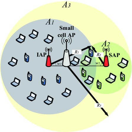
  Figure 1: The system model for CSCS

• The area of $A_{1}$, $A_{2}$, and $A_{3}$ are, respectively, $S_{A_{1}}$, $S_{A_{2}}$, and $S_{A_{3}}$. The area of overlap between $A_{1}$ and $A_{2}$ is $S_{A_{1}\cap A_{2}}$.

• $S_{A_{3}}$ is relatively large. $S_{A_{1}\cap A_{2}}$ is relatively small.

• Inhabitants and sojourners are uniformly distributed in their respective activity areas. The number of users is relatively large.

• The inhabitants have higher status.

• ISSC and SSSC are respectively consistent with the inhabitants’ activity area $A_{1}$ and the sojourners’ activity area $A_{2}$.

II-B Cognitive Sub-Small Cell for Sojourners

CSCS turns the single small cell into two sub-small cells: Inhabitant Sub-Small Cell (ISSC) and Sojourner Sub-Small Cell (SSSC), each of which is served by its own AP. ISSC serves the inhabitants by Inhabitant Access Point (IAP). SSSC serves the sojourners by Sojourner Access Point (SAP). Both IAP and SAP exploit BD precoding and full rank transmission. The sub-small cells use the same number of subcarriers and the same spectrum as that are used by the small cell AP. We assume that both sub-small cell APs take inhabitants and sojourners in their respective coverage area into account to design BD precoding.

II-C Number of Concurrent Sojourners

Our analysis for SSSC is based on the following assumptions:

• Sojourners arrive SSSC according to a time-varing Poisson process with arrival rate $\lambda\left(t\right)$ and $N_{2}\left(t=0\right)=0$.

• The duration of stay of one sojourner is modeled as a duration of a continuous time Markov process with $m+1$ states from its starting until its ending in the absorbing state, where $m\geq 1$. The probability of this process starting in the state $i$ is $\alpha_{i}$, where $i=1,\ldots,m+1$. The state $m+1$ is the absorbing state and the others are transient states. We assume that this process will never start in the absorbing state, i.e. $\alpha_{m+1}=0$.

The duration of stay of one sojourner has a phase-type distribution [18]. We denote by $\mathbf{R}$ the matrix which contains the transition rates among the transient states. $\mathbf{R}$ is a matrix of size $m\times m$. The duration of stay of one sojourner is denoted by $X$. The Cumulative Distribution Function (CDF) of $X$ is given by

$$F_{X}\left(x\right)=1-\boldsymbol{\alpha}\exp\left(\mathbf{R}x\right)\mathbf{1},\;x\geq 0,$$ (1)

where $\boldsymbol{\alpha}=\left[\alpha_{1},\ldots,\alpha_{m}\right]$, $\exp\left(\bullet\right)$ is the matrix exponential and $\mathbf{1}$ is an $m\times 1$ vector with all elements equal to 1.

Remark 1.

Under the above assumptions, SSSC can be modeled as an $M_{t}/G/\infty$ queue with service time follows a phase type distribution, arrival rate $\lambda\left(t\right)$ and $N_{2}\left(t=0\right)=0$. Authors in [19] have given the probability distribution of the number of concurrent users in such queueing system. Accordingly, $N_{2}\left(t\right)$ has a Poisson distribution with parameter

$$v\left(t\right)=\int_{0}^{t}\lambda\left(\tau\right)\left[1-F_{X}\left(t-\tau\right)\right]d\tau,\;t\geq 0.$$ (2)

The Probability Mass Function (PMF) of $N_{2}\left(t\right)$ is

$$f_{N_{2}\left(t\right)}\left(n\right)=\mathbb{P}\left(N_{2}\left(t\right)=n\right)=\frac{\left[v\left(t\right)\right]^{n}}{n!}\exp\left(-v\left(t\right)\right),$$ (3)

where $n\in\mathbb{Z}_{0}^{+}$.

The CDF of $N_{2}\left(t\right)$ is

$$F_{N_{2}\left(t\right)}\left(n^{\prime}\right)=\sum_{n=0}^{n^{\prime}}f_{N_{2}\left(t\right)}\left(n\right),$$ (4)

where $n^{\prime}\in\mathbb{Z}_{0}^{+}$.

II-D Downlink inter-sub-small cell interference

Due to BD precoding, ISSC and SSSC will not cause downlink inter-sub-small cell interference when perfect IAP-to-sojourner CSI and SAP-to-inhabitant CSI are acquired by IAP and SAP respectively.

Remark 2.

In practice, the perfect acquisition of SAP-to-inhabitant CSI is hampered by the lack of explicit coordination and full cooperation between ISSC and SSSC, since inhabitants are scant of willingness to feedback SAP-to-inhabitant CSI by using their own bandwidth and power. SAP has to turn to blind CSI estimate or other inexact CSI estimates which will furnish imperfect SAP-to-inhabitant CSI [14, 15]. Therefore, the root cause of interference inflicted by SSSC on ISSC is uncertain SAP-to-inhabitant CSI.

In this paper, the interference inflicted by ISSC on SSSC is not a key focus of our study. We make the assumption that either sojourners are willing to feedback IAP-to-sojourner CSI by using their own bandwidth and power to avoid interference owing to perfect IAP-to-sojourner CSI, or sojourners will not access the spectrum which is heavily used by the inhabitants.

Since the IAP-to-inhabitant CSI and SAP-to-sojourner CSI are perspicuous for IAP and SAP, there is no interference inside ISSC or SSSC in our system. In some relevant papers about underlay multicarrier cognitive radio systems with uncertain CSI, the subcarrier scheduling is the way for steering clear of the interference inside the secondary systems [20, 21].

III Determining Number of Transmit Antennas on Sub-small Cell Access Points

BD precoding and full rank transmission requires that the number of transmit antennas is not less than the total number of receive antennas. Therefore, the number of concurrently supportable users is limited by the number of transmit antennas. When the number of users is greater than the number of concurrently supportable users, AP will select users to simultaneously serve using some kind of user selection algorithm.

QoS requirements and the number of users who simultaneously present make demands on the number of concurrently supportable users.

In our system, we express the required number of concurrently supportable sojourners as $N_{2}\left(t\right)Q$, where $Q$ indicates the minimum QoS requirements of sojourners, $Q\leq 1$, and $N_{2}\left(t\right)Q\in\mathbb{Z}^{+}$.

In this paper, we investigate the issue of determining the number of transmit antennas under the premise that AP can support the installation of selected number of transmit antennas.

We put forward a criterion to determine an appropriate number of transmit antennas on Sub-small Cell Access Points:

• It pursues the minimum number of transmit antennas which ensures BD and full rank transmission to be validated.

• It ensures that the mean value of the probability of the number of concurrently supportable sojourners being adequate during an applicable period is no less than the predetermined probability or the growth of this mean value of probability led by adding one more supportable sojourner is less than a threshold.

We denote by $N_{U}$ the number of concurrently supportable sojourners. For our system, the probability of the number of concurrently supportable sojourners being adequate at time $t$ is

$$P\left(N_{U},\;t\right)=F_{N_{2}\left(t\right)}\left(N_{U}/Q\right).$$ (5)

We define the mean value of the probability of the number of concurrently supportable sojourners being adequate during the time interval $\left[0,\;T\right]$ as

$$E\left[P\left(N_{U},\;t\right)\right]=\frac{1}{T}\int_{t=0}^{T}P\left(N_{U},\;t\right)dt.$$ (6)

According to the first item of our criterion, we have

$$N_{U}=N_{ST}/N_{R}-N_{1}^{{}^{\prime}},$$ (7)

where $N_{ST}$ is the possible number of transmit antennas on SAP and $N_{U}\in\mathbb{Z}^{+}$.

Proposition 1.

The number of transmit antennas on sub-small cell APs can be determined as follows:

Since $N_{R}$ and $N_{1}^{{}^{\prime}}$ are supposed to be known in our system model, the selected number of transmit antennas on SAP $N_{ST}^{*}$ is determined by (8) or (9):

$$N_{ST}^{*}=\min_{N_{ST}}\left\{E\left[P\left(N_{U},\;t\right)\right]\geq\eta\right\},$$ (8)

$$N_{ST}^{*}=\min_{N_{ST}}\left\{E\left[P\left(N_{U}+1,\;t\right)\right]-E\left[P\left(N_{U},\;t\right)\right]\leq\gamma\right\},$$ (9)

where $\eta$ is a predetermined probability and $\gamma$ is a threshold.

We denote by $N_{IT}$ the selected number of transmit antennas on IAP. $N_{IT}$ is determined by

$$N_{IT}=N_{R}Q^{\prime}\left(N_{1}+\frac{N_{U}^{*}S_{A_{1}\cap A_{2}}}{S_{A_{2}}}\right).$$ (10)

where $N_{U}^{*}=N_{ST}^{*}/N_{R}-N_{1}^{{}^{\prime}}$ and $Q^{\prime}$ indicates the QoS requirements of inhabitants.

IV Downlink Inter-sub-small Interference Control

As discussed above, for our system, due to the use of BD, no inter-sub-small cell interference is caused by downlink transmission under the situation that IAP and SAP acquire perfect IAP-to-sojourner CSI and SAP-to-inhabitant CSI respectively. However, the interference inflicted by SSSC on ISSC has its origins in BD precoding exploiting CSI with inevitable uncertainty. We proposed an interference control scheme named BDBF for secondary systems which are hampered from perfect secondary-to-primary CSI. BDBF utilizes BD Precoding based on uncertain CSI in conjunction with auxiliary optimal BF. In view of the adoption of OFDM, we turn the design of auxiliary optimal BF of BDBF into a multi-user multi-subcarrier optimal BF design under channel uncertainties. For such optimization problems that contain the uncertainty region constraint, S-Procedure is an efficacious tool to transform semi-infinite programs into equivalent semi-definite programs [15, 20]. We prove and verify that BDBF performs better than the interference controller using optimal BF alone for gaining more capacity within a bearably large radius of uncertainty region.

IV-A Block Diagonalization

For each user $u_{i}$, BD algorithm [10] constructs a precoding matrix $\mathbf{W}_{t,u_{i},s}$ which achieves the zero-interference constraint, i.e.

$$\mathbf{H}_{t,u_{j},s}\mathbf{W}_{t,u_{i},s}=0,\,\forall j\neq i,$$ (11)

where $\mathbf{H}_{t,u_{j},s}\in N_{r}\times N_{t}$ denotes the channel matrix from transmitter $t$ to user $u_{j}$ at subcarrier $s$, $N_{r}$ denotes the number of receive antennas at every UE and $N_{t}$ denotes the number of transmit antennas at transmitter $t$.

Suppose that $N_{u}$ users are within the coverage area of transmitter $t$ and we define

$$\tilde{\mathbf{H}}_{t,u_{i},s}=\left[\mathbf{H}_{t,u_{1},s}^{T}\ldots\mathbf{H}_{t,u_{i-1},s}^{T}\;\mathbf{H}_{t,u_{i+1},s}^{T}\ldots\mathbf{H}_{t,u_{N_{u}},s}^{T}\right]^{T}.$$ (12)

Hereupon, Equation (11) has another equivalent form

$$\tilde{\mathbf{H}}_{t,u_{i},s}\mathbf{W}_{t,u_{i},s}=0.$$ (13)

From Equation (13), it is deduced that $\mathbf{W}_{t,u_{i},s}$ is a basis set in the null space of $\tilde{\mathbf{H}}_{t,u_{i},s}$. The Singular Value Decomposition (SVD) of $\tilde{\mathbf{H}}_{t,u_{i},s}$ is expressed as

$$\tilde{\mathbf{H}}_{t,u_{i},s}=\mathbf{\tilde{U}}_{t,u_{i},s}\left[\tilde{\boldsymbol{\Lambda}}_{t,u_{i},s}\mathbf{0}\right]\left[\mathbf{\tilde{V}}_{t,u_{i},s}^{\left(1\right)}\mathbf{\tilde{V}}_{t,u_{i},s}^{\left(0\right)}\right]^{\mathcal{H}},$$ (14)

where $\mathbf{\tilde{V}}_{t,u_{i},s}^{\left(0\right)}\in\mathbb{C^{\mathrm{\mathit{\mathrm{N_{t}\times\left(N_{t}-rank\left(\mathbf{\tilde{H}}_{\mathit{t,u_{i},s}}\right)\right)}}}}}$ contains the right-singular vectors corresponding to the zero singular values of $\mathbf{\tilde{H}}_{t,u_{i},s}$, i.e. $\mathbf{\tilde{V}}_{t,u_{i},s}^{\left(0\right)}$ forms a null space basis of $\mathbf{\tilde{H}}_{t,u_{i},s}$. Therefore $\mathbf{W}_{t,u_{i},s}$ can be constructed by any linear combinations of the columns in $\mathbf{\tilde{V}}_{t,u_{i},s}^{\left(0\right)}$. Correspondingly, $\mathbf{H}_{t,u_{i},s}\mathbf{\tilde{V}}_{t,u_{i},s}^{\left(0\right)}$ forms the equivalent channel.

The SVD precoding can be performed using the equivalent channel:

$$\mathbf{H}_{t,u_{i},s}\mathbf{\tilde{V}}_{t,u_{i},s}^{\left(0\right)}=\mathbf{U}_{t,u_{i},s}\left[\begin{array}[]{cc}\boldsymbol{\Lambda}_{t,u_{i},s}&\mathbf{0}\\ \mathbf{0}&\mathbf{0}\end{array}\right]\left[\mathbf{V}_{t,u_{i},s}^{\left(1\right)}\mathbf{V}_{t,u_{i},s}^{\left(0\right)}\right]^{\mathcal{H}},$$ (15)

where $\mathbf{V}_{t,u_{i},s}^{\left(1\right)}\in\mathbb{C^{\mathrm{\mathit{\mathrm{\left(N_{t}-rank\left(\mathbf{\tilde{H}}_{\mathit{t,u_{i},s}}\right)\right)\times rank\left(\mathbf{H}_{t,u_{i},s}\mathbf{\tilde{V}}_{t,u_{i},s}^{\left(0\right)}\right)}}}}}$ contains the right-singular vectors corresponding to the non-zero singular values of $\mathbf{H}_{t,u_{i},s}\mathbf{\tilde{V}}_{t,u_{i},s}^{\left(0\right)}$. $\mathbf{V}_{t,u_{i},s}^{\left(1\right)}$ is used as SVD precoder and $\mathbf{U}_{t,u_{i},s}^{\mathcal{H}}$ is used as SVD decoder. Consequently, the precoding matrix $\mathbf{W}_{t,u_{i},s}$ can be chosen as $\mathbf{\tilde{V}}_{t,u_{i},s}^{\left(0\right)}\mathbf{V}_{t,u_{i},s}^{\left(1\right)}$.

For the full rank transmission, i.e. the number of streams sent to a UE is no less than the number of receive antennas, it is needed that $N_{t}-\mathrm{rank}\left(\tilde{\mathbf{H}}_{t,u_{i},s}\right)\geq N_{r}$, i.e. $N_{t}\geq N_{r}\mathit{N}_{u}$. In this paper, we consider the situation that the number of streams sent to a UE equals the number of receive antennas, i.e $N_{t}=N_{r}N_{u}$. Accordingly, $\mathbf{W}_{t,u_{i},s}$ is a matrix of size $N_{t}\times N_{r}$.

IV-B BDBF

As explained in Remark 1, SAP-to-inhabitant CSI is unable to be perfect. The SAP-to-inhabitant channel matrix at subcarrier $s$ can be expressed as

$$\mathbf{H}_{SAP,I_{i},s}=\hat{\mathbf{H}}_{SAP,I_{i},s}+\mathbf{\triangle\mathbf{H}_{\mathit{SAP,I_{i},s}}},$$ (16)

where $\hat{\mathbf{H}}_{SAP,I_{i},s}$ is the estimated channel matrix from transmitter $SAP$ to user $I_{i}\in U_{I}^{{}^{\prime}}$ at subcarrier $s$ and $\mathbf{\triangle\mathbf{H}_{\mathit{SAP,I_{i},s}}}$ is the channel uncertainty matrix from transmitter $SAP$ to user $I_{i}\in U_{I}^{{}^{\prime}}$ at subcarrier $s$. In this paper, we adopt a channel uncertainty model [22] which defines the uncertainty region as

$$\triangle\left(\epsilon\right)=\left\{\triangle\mathbf{H}_{\mathit{SAP,I_{i},s}}\mid\mathrm{Tr}\left\{\mathbf{E}\right\}\leq\epsilon^{2}\right\},$$ (17)

where $\mathbf{E=\triangle\mathbf{H}_{\mathit{SAP,I_{i},s}}}\mathbf{\mathbf{\triangle\mathbf{H}_{\mathit{SAP,I_{i},s}}^{\mathit{\mathcal{H}}}}}$.

Proposition 2.

For secondary systems which are hampered from perfect secondary-to-primary CSI, secondary systems can exploit BDBF: BD precoding based on uncertain CSI in conjunction with auxiliary optimal BF to control interference to primary systems.

After BDBF, the transmitted signal from SAP to sojourner $S_{i}$ can be expressed as

$$\mathbf{S}_{SAP,S_{i},s}=\mathbf{W}_{SAP,S_{i},s}\mathbf{P}_{SAP,S_{i},s}\mathbf{x}_{SAP,S_{i},s}$$ (18)

where

$\mathbf{x}_{SAP,I_{i},s}\in\mathbb{C}^{N_{ST}^{*}\times 1}$ is the information symbol vector transmitted from SAP to $I_{i}$ at subcarrier $s$ with covariance matrix $\mathbb{E}\left\{\mathbf{x}_{SAP,I_{i},s}\mathbf{x}_{SAP,I_{i},s}^{\mathcal{H}}\right\}=\mathbf{I}_{N_{ST}^{*}}$,

$\mathbf{P}_{SAP,I_{i},s}\in\mathbb{C}^{N_{R}\times N_{ST}^{*}}$ is the auxiliary optimal BF,

and $\mathbf{W}_{SAP,S_{i},s}$ is the BD precoding matrix of size $N_{ST}^{*}\times N_{R}$.

$\mathbf{W}_{SAP,S_{i},s}$ is generated by $\tilde{\mathbf{H}}_{SAP,S_{i},s}=\left[\breve{\mathbf{H}}_{SAP,S_{i},s}\;\mathbf{H}_{SAP,I_{1},s}^{T}\ldots\mathbf{H}_{SAP,I_{N_{1}},s}^{T}\right]^{T}$ and $\breve{\mathbf{H}}_{SAP,S_{i},s}=\left[\mathbf{H}_{SAP,S_{1},s}^{T}\ldots\mathbf{H}_{SAP,S_{i-1},s}^{T}\;\mathbf{H}_{SAP,S_{i+1},s}^{T}\ldots\mathbf{H}_{SAP,S_{N_{2}\left(t\right)},s}^{T}\right]$.

For inhabitant $I_{i}$, the received signal at subcarrier $s$ is given by

$$\mathbf{y}_{I_{i},s} = \mathbf{U}_{IAP,I_{i},s}^{\mathcal{H}}\mathbf{H}_{IAP,I_{i},s}\mathbf{W}_{IAP,I_{i},s}\mathbf{x}_{IAP,I_{i},s}$$ (19)

$$+ \sum_{S_{i}\in U_{S}}\mathbf{H}_{SAP,I_{i},s}\mathbf{W}_{SAP,S_{i},s}\mathbf{P}_{SAP,S_{i},s}\mathbf{x}_{SAP,S_{i},s}$$

$$+ \mathbf{n}_{I_{i},s},$$

where

$\mathbf{x}_{IAP,I_{i},s}\in\mathbb{C}^{N_{IT}\times 1}$ is the information symbol vector transmitted from $IAP$ to $I_{i}$ at subcarrier $s$ with covariance matrix $\mathbb{E}\left\{\mathbf{x}_{IAP,I_{i},s}\mathbf{x}_{IAP,I_{i},s}^{\mathcal{H}}\right\}=\mathbf{I}_{N_{IT}}$,

$\mathbf{n}_{I_{i},s}\in\mathbb{C}^{N_{R}\times 1}$ is the i.i.d. circularly symmetric white Gaussian noise at subcarrier $s$ at reciever $I_{i}$ with covariance matrix $\mathbb{E}\left\{\mathbf{n}_{I_{i},s}\mathbf{n}_{I_{i},s}^{\mathcal{H}}\right\}=\mathbf{I}_{N_{R}}$,

$\mathbf{W}_{IAP,I_{i},s}$ is the BD precoding matrix of size $N_{IT}\times N_{R}$,

and $\mathbf{U}_{IAP,I_{i},s}^{\mathcal{H}}$ is the SVD decoding matrix of size $N_{R}\times N_{R}$.

$\mathbf{W}_{IAP,I_{i},s}$ and $\mathbf{U}_{IAP,I_{i},s}^{\mathcal{H}}$ are generated by $\tilde{\mathbf{H}}_{IAP,I_{i},s}=\left[\mathbf{\overline{H}}_{IAP,I_{i},s}\;\mathbf{H}_{IAP,S_{1},s}^{T}\ldots\mathbf{H}_{IAP,S_{N_{2}(t)},s}^{T}\right]^{T}$ and $\mathbf{\mathbf{\overline{H}}}_{IAP,I_{i},s}=\left[\mathbf{H}_{IAP,I_{1},s}^{T}\ldots\mathbf{H}_{IAP,I_{i-1},s}^{T}\;\mathbf{H}_{IAP,I_{i+1},s}^{T}\ldots\mathbf{H}_{IAP,I_{N_{1}},s}^{T}\right]$.

Theorem 1.

The auxiliary optimal BF of BDBF can be formulated as the following multi-user multi-subcarrier optimal BF design under channel uncertainties: trying for the maximum capacity of secondary system under the precondition that the interference inflicted to the primary system is kept below the threshold.

$$\left(\mathbf{\mathrm{\mathbf{P1}}}\right)\;\max_{\boldsymbol{Q}_{SAP,S_{i},s}}\sum_{s=1}^{N_{C}}\sum_{S_{i}\in U_{S}}\log\mathrm{det}\left(\mathbf{\mathbf{I}_{\mathit{N_{R}}}}+\frac{SNR}{N_{ST}^{*}}\mathbf{A}\right)$$ (20a)

$$\mathrm{s.t.}\;\boldsymbol{Q}_{SAP,S_{i},s}\geqslant 0,\;\forall S_{i}\in U_{S},\;\forall s,$$ (20b)

$$\sum_{S_{i}\in U_{S}}\mathrm{Tr}\left(\boldsymbol{\breve{Q}}_{SAP,S_{i},s}\right)\leq P_{SAP},\;\forall S_{i}\in U_{S},\;\forall s,$$ (20c)

$$\mathrm{Tr}\left(\mathbf{B}\right)\leq\zeta,\;\forall\triangle\mathrm{\mathbf{H}}_{SAP,I_{i},s}\in\triangle\left(\epsilon\right),\;\forall S_{i}\in U_{S},\;\forall I_{i}\in U_{I}^{{}^{\prime}},\;\forall s,$$ (20d)

where

$\boldsymbol{Q}_{SAP,S_{i},s}=\mathbf{P}_{SAP,S_{i},s}\mathbf{P}_{SAP,S_{i},s}^{\mathcal{H}},$

$\boldsymbol{\breve{Q}}_{SAP,S_{i},s}=\mathbf{W}_{SAP,S_{i},s}\boldsymbol{Q}_{SAP,S_{i},s}\mathbf{\mathbf{W}_{\mathit{SAP,S_{i},s}}^{\mathcal{H}}},$

$\mathbf{A}=\boldsymbol{\Lambda}_{SAP,S_{i},s}\boldsymbol{Q}_{SAP,S_{i},s}\mathrm{\mathbf{\boldsymbol{\Lambda}}}_{SAP,S_{i},s}^{\mathcal{H}},$

$\mathbf{B}=\mathrm{\mathbf{H}}_{SAP,I_{i},s}\boldsymbol{\breve{Q}}_{SAP,S_{i},s}\mathrm{\mathbf{H}}_{SAP,I_{i},s}^{\mathcal{H}},$

$P_{SAP}$ is the maximum downlink transmit power of SAP,

and $\zeta$ is the inter-sub-small interference tolerable threshold on each subcarrier for inhabitant $I_{i}\in U_{I}^{{}^{\prime}}$.

$\boldsymbol{Q}_{SAP,S_{i},s}$ is a positive semidefinite matrix to render certain that the elements on the main diagonal of $\mathbf{A}$ and $\mathbf{B}$ are real and non-negative. Additionally, $\boldsymbol{Q}_{SAP,S_{i},s}$ is a symmetric matrix to ensure that linear matrix inequality (LMI) holds.

$\triangle\left(\epsilon\right)$ is a set of infinite cardinality and accordingly the inequality (20d) imposes infinite constraints. This means that $\left(\mathrm{P1}\right)$ is a semi-infinite program. $\left(\mathrm{P1}\right)$ can be transformed into an equivalent semi-definite program $\left(\mathrm{P2}\right)$ with the constraint (21g) which contains finite constraints instead of the constraint (20d):

$$\left(\boldsymbol{\mathbf{\mathbf{\mathrm{P2}}}}\right)\;\max_{\boldsymbol{Q}_{SAP,S_{i},s}}\sum_{s=1}^{N_{C}}\sum_{S_{i}\in U_{S}}\log\mathrm{det}\left(\mathbf{\mathbf{I}_{\mathit{N_{R}}}}+\frac{SNR}{N_{ST}^{*}}\mathbf{A}\right)$$ (21a)

$$\mathrm{s.t.}\;\boldsymbol{Q}_{SAP,S_{i},s}\geqslant 0,\;\forall S_{i}\in U_{S},\;\forall s,$$ (21b)

$$\sum_{S_{i}\in U_{S}}\mathrm{Tr}\left(\boldsymbol{\breve{Q}}_{SAP,S_{i},s}\right)\leq P_{SAP},\;\forall S_{i}\in U_{S},\;\forall s,$$ (21c)

$$\left[\begin{array}[]{cc}\alpha\mathbf{\mathbf{I}}_{N_{T}\times N_{R}}+\mathbf{G}&\mathbf{J}^{\mathcal{H}}\\ \mathbf{J}&k-\alpha\epsilon^{2}\end{array}\right] \geq 0,$$ (21f)

$$\forall\alpha\geq 0,\;\forall I_{i}\in U_{I}^{{}^{\prime}},\;\forall S_{i}\in U_{S},\;\forall s$$ (21g)

Proof:

According to the relationship between the trace operator and the vec operator $\mathrm{Tr}\left(\mathbf{C^{\mathcal{H}}DC}\right)=\mathrm{vec}\left(\mathbf{C}\right)^{\mathcal{H}}\left(\mathbf{I}\otimes\mathbf{D}\right)\mathrm{vec}\left(\mathbf{C}\right)$ and $\mathrm{Tr}\left(\mathbf{C^{\mathcal{H}}D}\right)=\mathrm{vec}\left(\mathbf{C}\right)^{\mathcal{H}}\mathrm{vec}\left(\mathbf{D}\right)$, the inequality (20d) can be converted to an equivalent form:

$$-vec\left(\mathbf{\mathrm{\triangle}\mathbf{H}_{\mathit{SAP,I_{i},s}}^{\mathit{\mathcal{H}}}}\right)^{\mathit{\mathcal{H}}}\left(\mathbf{I}_{N_{R}}\otimes\boldsymbol{\breve{Q}}_{SAP,S_{i},s}\right)vec\left(\mathbf{\mathrm{\triangle}\mathbf{H}_{\mathit{SAP,I_{i},s}}^{\mathit{\mathcal{H}}}}\right)$$

$$-2\mathfrak{R}\left(\mathrm{vec}\left(\mathbb{\mathbf{\boldsymbol{\breve{Q}}_{\mathit{SAP,S_{i},s}}}^{\mathit{\mathcal{H}}}}\mathbf{\mathbf{\hat{H}}_{\mathit{SAP,I_{i},s}}^{\mathit{\mathcal{H}}}}\right)^{\mathcal{H}}\mathrm{vec}\left(\mathrm{\triangle}\mathbf{H}_{\mathit{SAP,I_{i},s}}^{\mathit{\mathcal{H}}}\right)\right)$$

$$-\mathrm{Tr}\left(\mathbf{\mathbf{\hat{H}}_{\mathit{SAP,I_{i},s}}\mathbf{\boldsymbol{\breve{Q}}_{\mathit{SAP,S_{i},s}}}}\mathbf{\mathbf{\hat{H}}_{\mathit{SAP,I_{i},s}}^{\mathit{\mathcal{H}}}}\right)$$

$$+\zeta\geq 0,$$

$$\forall vec\left(\mathbf{\mathrm{\mathrm{\triangle}}\mathbf{H}_{\mathit{SAP,I_{i},s}}^{\mathit{\mathcal{H}}}}\right)^{\mathit{\mathcal{H}}}vec\left(\mathbf{\mathrm{\triangle}\mathbf{H}_{\mathit{SAP,I_{i},s}}^{\mathit{\mathcal{H}}}}\right)\leq\epsilon^{2},$$

$$\forall I_{i}\in U_{I}^{{}^{\prime}},\;\forall S_{i}\in U_{S},\;\forall s$$ (22)

The result of S-Procedure [23, 24] presents a condition that makes the infinite constraints imposed by the inequality (22) hold: if and only if there exists $\alpha\geqslant 0$ such that the inequality (23) is ture.

$$\left[\begin{array}[]{cc}\alpha\mathbf{\mathbf{I}}_{N_{T}\times N_{R}}+\mathbf{G}&\mathbf{J}^{\mathcal{H}}\\ \mathbf{J}&k-\alpha\epsilon^{2}\end{array}\right]\geq 0,\;\forall I_{i}\in U_{I}^{{}^{\prime}},\;\forall S_{i}\in U_{S},\;\forall s$$ (23)

where $\mathbf{G}=-\mathbf{\mathbf{I}}_{N_{R}}\otimes\boldsymbol{\breve{Q}}_{SAP,S_{i},s}$, $\mathbf{J}=-\mathrm{vec}\left(\mathbb{\mathbf{\boldsymbol{\breve{Q}}}_{\mathit{SAP,S_{i},s}}^{\mathit{\mathcal{H}}}}\mathbf{\mathbf{\hat{H}}_{\mathit{SAP,I_{i},s}}^{\mathit{\mathcal{H}}}}\right)$, and $k=\zeta-\mathrm{Tr}\left(\mathbf{\mathbf{\hat{H}}_{\mathit{SAP,I_{i},s}}}\boldsymbol{\breve{Q}}_{SAP,S_{i},s}\mathbf{\mathbf{\hat{H}}_{\mathit{SAP,I_{i},s}}^{\mathit{\mathcal{H}}}}\right)$. ∎

The semi-definite program $\left(\mathrm{P2}\right)$ can be solved by interior point methods [24, 25].

Theorem 2.

BDBF can gain more capacity than the interference controller that using optimal BF alone within a bearably large radius of uncertainty region.

Proof:

We denote by $\mathbf{W}_{SAP,S_{i},s}^{a}$ and $\mathbf{W}_{SAP,S_{i},s}^{b}$ the BD precoding matrix which is generated by $\tilde{\mathbf{H}}_{SAP,S_{i},s}^{a}=\left[\breve{\mathbf{H}}_{SAP,S_{i},s}\;\mathbf{\hat{H}}_{IAP,I_{1},s}^{T}\ldots\mathbf{\hat{H}}_{IAP,I_{N_{1}},s}^{T}\right]^{T}$ and the BD precoding matrix which is generated by $\tilde{\mathbf{H}}_{SAP,S_{i},s}^{b}=\left[\breve{\mathbf{H}}_{SAP,S_{i},s}\right]^{T}$, respectively. Since $\mathbf{W}_{SAP,S_{i},s}^{a}$ is a basis set in the null space of $\tilde{\mathbf{H}}_{SAP,S_{i},s}^{a}$, then for $\epsilon^{2}\leq\iota$, we have $\mathrm{Tr}\left(\mathrm{\mathbf{H}}_{SAP,I_{i},s}\mathbf{W}_{SAP,S_{i},s}^{a}\mathbf{W}_{SAP,S_{i},s}^{\mathcal{\mathit{a}H}}\mathrm{\mathbf{H}}_{SAP,I_{i},s}^{\mathcal{H}}\right)<\mathrm{Tr}\left(\mathrm{\mathbf{H}}_{SAP,I_{i},s}\mathbf{W}_{SAP,S_{i},s}^{b}\mathbf{W}_{SAP,S_{i},s}^{\mathcal{\mathit{b}H}}\mathrm{\mathbf{H}}_{SAP,I_{i},s}^{\mathcal{H}}\right)$, where $\iota$ is a constant. Accordingly, for $\epsilon^{2}\leq\iota$, when $\mathrm{Tr}\left(\mathbf{B}^{a}\right)=\mathrm{Tr}\left(\mathbf{B}^{b}\right)=\zeta$, we have $\mathrm{Tr}\left(\boldsymbol{Q}_{SAP,S_{i},s}^{a}\right)>\mathrm{Tr}\left(\boldsymbol{Q}_{SAP,S_{i},s}^{b}\right)$, where $\mathbf{B}^{a}=\mathrm{\mathbf{H}}_{SAP,I_{i},s}\mathbf{W}_{SAP,S_{i},s}^{a}\boldsymbol{Q}_{SAP,S_{i},s}^{a}\mathbf{W}_{SAP,S_{i},s}^{\mathcal{\mathit{a}H}}\mathrm{\mathbf{H}}_{SAP,I_{i},s}^{\mathcal{H}}$ and $\mathbf{B}^{b}=\mathrm{\mathbf{H}}_{SAP,I_{i},s}\mathbf{W}_{SAP,S_{i},s}^{b}\boldsymbol{Q}_{SAP,S_{i},s}^{b}\mathbf{W}_{SAP,S_{i},s}^{\mathcal{\mathit{b}H}}\mathrm{\mathbf{H}}_{SAP,I_{i},s}^{\mathcal{H}}$. Therefore, for $\epsilon^{2}\leq\iota$, based upon Theorem 1., the capacity of SSSC using $\mathbf{W}_{SAP,S_{i},s}^{a}$ is larger than that of SSSC using $\mathbf{W}_{SAP,S_{i},s}^{b}$. ∎

We simulate the SSSC using $\mathbf{W}_{SAP,S_{i},s}^{a}$ and $\mathbf{W}_{SAP,S_{i},s}^{b}$ for different $\epsilon^{2}$ in Section IV. We find that $\iota$ can be much larger than the normally acceptable radius of uncertainty region.

V Simulation

V-A Number of Transmit Antennas on Sub-small Cell Access Points

Since the number of transmit antennas on SAP and that on IAP are in direct relation with the number of concurrent sojourners, we design 8 data sets to observe and analyze the number of concurrent sojourners in 8 representative circumstances.

We consult a medium-sized software enterprise in Paris to help us to design data sets to approximate the actual situation. We receive the following information on visitors in this enterprise:

• There are more than fifty visitors daily at an average.

• In view of long term observation, there is no such a working day when the number of visitors is particularly large or small within five working days.

• After the holidays, the number of visitors is inclined to peak.

First, we exclude those days when the number of visitors is inclined to peak after holidays. Based on the second item above, we consider that the observations of the number of arrivals at the reference time on different working days are independent and identically distributed (i.i.d.). We observe the sample mean of the cumulative probability of the number of concurrent sojourners during one entire working day based on the first six data sets. Here, we set $Q=1$. We adopt $E\left[P\left(N_{U},\;t\right)\right]$ which is defined in Equation (6) to indicate the sample mean of the cumulative probability of the number of concurrent sojourners during the observation time interval. We interpret $P\left(N_{U},\;t\right)$ as the probability of the number of concurrent sojourners being less than $N_{U}$ at time $t$.

Then we consider separately those days after holidays. We also consider that the observations of the number of arrivals at the reference time on different working days during those days are i.i.d.. We observe the sample mean of the cumulative probability of the number of concurrent sojourners during one entire working day based on the last two data sets.

We list the attributes of these 8 test data sets in Table (II).

TABLE II: Attributes of test data sets

Data set index
Observation time interval (9 am to 5 pm)
Total number of sojourners during the observation time interval
Sample mean of the duration of stay of one sojourner (minute)
Standard deviation of the duration of stay of one sojourner
Arrival rate (arrivals per time slot)
Data set 1	Data set 2	Data set 3	Data set 4
-	-	-	-
60	60	60	60
60	60	90	90
3.7947	148.0447	3.7947	148.0447
60/48	60/48	60/48	60/48
Data set 5	Data set 6	Data set 7	Data set 8
-	-	-	-
60	60	90	90
60	60	60	60
3.7947	148.0447	2.7809	134.5144
5(10-11 am), 30/42(else)	5(10-11 am), 30/42(else)	60/48	60/48

The staffs’ working hours are from 9 am to 5 pm. The visitors arrive randomly during working hours. The observation time interval is set to be consistent with the working hours for all data sets. We divide the observation time interval into $48$ time slots, each $10$ minutes in length. Data set 1 and data set 2 have the same attributes except the standard deviation of the duration of stay. These two data sets are considered as the benchmark for comparison and designing the other data sets. Data set 3 and data set 4 are designed by adding 30 minutes to every sample of the duration of stay in data set 1 and set 2. Data set 5 and data set 6 are designed by changing the immutable arrival rate of data set 1 and data set 2 to 5 arrivals per time slot during 10-11 am and 30/42 arrivals per time slot during the other working hours. Date set 7 and set 8 are designed by adding 30 to the total number of sojourners during the observation time interval of data set 1 and data set 2 and make the the standard deviation of the duration of stay of data set 7 and data set 8 to be close to that of data set 1 and data set 2 respectively.

We exploit EMPHT algorithm [26, 27] to fit the phase type distribution to the data of duration of stay in each data set. The EMPHT is an iterative maximum likelihood estimation algorithm which outputs the $m\times 1$ vector $\boldsymbol{\alpha}$ and $m\times m$ matrix $\mathbf{R}$. We chose the number of phases as 4, i.e. $m=4$. We acquire these two parameters based on each data set after sufficient iterations when the likelihood function reaches zero growth and accordingly obtain the CDF of the duration of stay for each data set.

We further calculate the mean value of the cumulative probability of the number of concurrent sojourners during the observation time interval base on each of these 8 data sets and showed them in Figure 2. From them, we can observe how the following factors influence the number of concurrent sojourners and further impact the number of transmit antennas on sub-small cell APs:

• the standard deviation of the duration of stay

• the mean of the duration of stay

• the distribution of arrival rate

• the total number of sojourners during the observation time interval

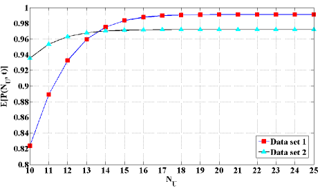
(a)

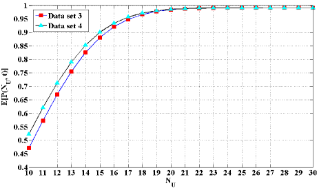
(b)

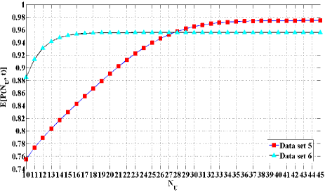
(c)

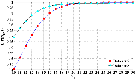
(d)

Figure 2: Sample mean of the CDF of the number of concurrent sojourners during the observation time interval base on each data set

From Figure 2, we observe that as $N_{U}$ increases, its sample mean of the cumulative probability of the number of concurrent sojourners during the observation time interval based on 8 data sets all exhibit uptrend and the rate of growth declines gradually. The values of $E\left[P\left(N_{U}=10,\;t\right)\right]$ based on data set 1 until data set 8 are: 0.8237, 0.9354, 0.4711, 0.5223, 0.7550, 0.8849, 0.4048 and 0.6905. The values of $E\left[P\left(N_{U}=20,\;t\right)\right]$ based on data set 1 until data set 8 are: 0.9911, 0.9719, 0.9841, 0.9857, 0.8908, 0.9554, 0.9852 and 0.9895. The pair of $n=\min_{N_{U}}\left\{E\left[P\left(N_{U}+1,\;t\right)\right]-E\left[P\left(N_{U},\;t\right)\right]\leq 0.001\right\}$ and $E\left[P\left(n,\;t\right)\right]$ based on data set 1 until data set 8 are: $(19,\;0.991)$, $\left(15,\;0.9712\right)$, $\left(24,\;0.9912\right)$, $\left(24,\;0.9911\right)$, $\left(38,\;0.9741\right)$, $\left(19,\;0.9553\right)$, $\left(26,\;0.9961\right)$ and $\left(22,\;0.9912\right)$.

From the first two sets of experimental results, we can observe that: the number of concurrent sojourners during the observation time interval being more than 20 has a very small probability (<0.03) for all data set 1, 2, 3, 4, 7 and 8 and a small probability (<0.11) for data set 5 and 6. This number being no more than 10 has a large probability (>0.8) for data set 1 and 2, followed by data set 5 and 6 (>0.75). For data set 3, 4, 7 and 8, This number being no more than 10 and between 10 and 20 have almost the same probability ($\approx 0.4$).

Referring to Figure 2, we can find that the increasement of the mean of the duration of stay, non-uniform arrival rate or the increase of the total number of sojourners during the observation time interval improves the probability of the number of concurrent sojourners being a relatively large number. The increasement of standard deviation of the duration of stay brings down this probability. However, when the mean of the duration of stay is relatively large, the standard deviation of the duration of stay has minimal impact on this probability as shown in Figure 2 (b). Accordingly, the number of transmit antennas on sub-small cell access points are chosen to be relatively large when the mean of the duration of stay or the total number of sojourners is relatively large, the arrival rate is non-uniform or the standard deviation of the duration of stay is relatively small.

From the third set of experimental result, we can see that the augmentation of standard deviation of the duration of stay causes that the convergence of the sample means of the cumulative probability of the number of concurrent sojourners during the observation time interval to be more slowly and the low growth rate emergences earlier. But when the mean of the duration of stay is relatively large, this phenomenon is not obvious. So we need to choose a relatively small value for $\eta$ in Equation (8) or $\gamma$ in Equation (9) when the standard deviation of the duration of stay is relatively large and the mean of the duration of stay is relatively small.

V-B BD precoding based on uncertain CSI in conjunction with auxiliary optimal BF for downlink inter-sub-small interference control

For simplicity we assume that the inter-sub-small cell interference only exists in the overlapping area between ISSC and SSSC in our simulation. We consider that 2 sojourners and 2 inhabitants stay in the overlap of ISSC and SSSC, where all the sojourners and inhabitants have the same distance from the SAP. The path loss component is normalized to one. $\mathrm{\mathbf{H}}_{SAP,S_{i},s}$ and $\mathbf{H}_{SAP,I_{i},s}$ are both modeled as a matrix with coefficients which are i.i.d. circularly symmetric, complex Gaussian random variables, with zero mean and unit variance. $\triangle\mathbf{H}_{\mathit{SAP,I_{i},s}}$ is modeled as a matrix with coefficients which are i.i.d. circularly symmetric, complex Gaussian random variables, with zero mean and variance $\sigma^{2}$. We set that $\epsilon^{2}$ in Equation (17) equals to $\sigma^{2}$. The number of receive antennas at every UE is set to be 2 and the maximum Signal-to-Noise Ratio (SNR) at every UE is set to be $20\,\mathrm{dB}$. The maximum downlink transmit power of SAP is 10W. The SAP exploits 4 subcarriers for downlink transmission. Each subcarrier occupies a normalized bandwidth of $1\,\mathrm{Hz}$.

For the purpose of comparing the performance of BDBF with the interference controller that uses optimal BF alone, we design two test systems: 1. downlink BD precoding for the secondary sub-small cell takes both sojourners and inhabitants who stay in the coverage area into consideration, i.e. the SSSC using $\mathbf{W}_{SAP,S_{i},s}^{a}$; 2. downlink BD precoding for the secondary sub-small cell takes only sojourners into consideration, i.e. the SSSC using $\mathbf{W}_{SAP,S_{i},s}^{b}$. We simulate the above systems which exploit BD precoding based on SAP-to-inhabitant CSI with different radius of uncertainty region ($\epsilon^{2}$=0, 0.1, 1, 5 and 10) and fed perfect SAP-to-inhabitant CSI to the optimal BF. We plot the average capacity of SSSC and the average interference to inhabitants on each subcarrier which are obtained by using 2000 Monte-Carlo realizations in Figure 3 and Figure 4 respectively.

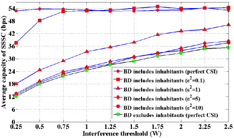
Figure 3: Average capacity of SSSC vs interference threshold

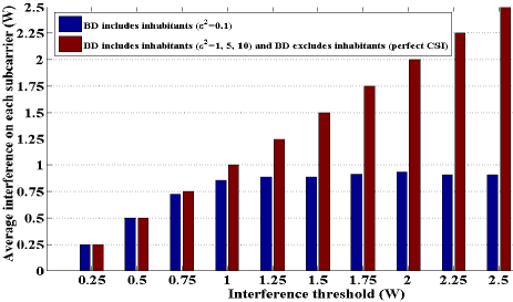
Figure 4: Average interference on each subcarrier vs. interference threshold

Figure 3 reveals the following information. 1. For the system adopts BD precoding including inhabitants, the average capacity of SSSC shakes off the shackles of interference threshold within the small radius of uncertainty region. For $\epsilon^{2}=0.1$, the average capacity of SSSC achieves 54.7651 bps when the interference threshold is 1.75W. After that it oscillates on small scale and no longer increases with the enhancement of threshold. This is because BD precoding based on uncertain CSI can inhibit the interference below the interference threshold within the small radius of uncertainty region. Figure 4 exhibits that the average interference to inhabitants on each subcarrier for $\epsilon^{2}=0.1$ is maintained below the threshold when the threshold is no less than 0.25W. For $\epsilon^{2}=0$, since BD precoding based on perfect CSI, the interference is completely eliminated and accordingly the average capacity of SSSC has no relationship with the interference threshold. It fluctuates slightly with the fluctuation of channel between SAP and sojourners. For $\epsilon^{2}=1,\;5,\;\mathrm{and}\;10$, the auxiliary optimal BF plays the leading role in inhibiting the interference. The actual interference is always equal to the threshold. The average capacity of SSSC exhibits uptrend as the threshold is enhanced. 2. System adopts BD precoding including inhabitants achieves higher capacity compared with that exploits BD precoding excluding inhabitants within a considerably large radius of uncertainty region. The average capacity of SSSC of the first system declines as the radius of uncertainty region increases. It should be noted that until $\epsilon^{2}$ increases to $10$, the average capacity of SSSC of the first system is still higher than that of the second system with $\epsilon^{2}=0$. This verifies Theorem 2.

VI Conclusion

In regard to design issues in CSCS, we put forward practical propositions for determining the number of transmit antennas and controlling downlink inter-sub-small cell interference. We found how the factors influence the number of concurrent sojourners and further impact the number of transmit antennas on sub-small cell APs. We proved and verified that BDBF performs better than the interference controller using optimal BF alone for gaining more capacity within a bearably large radius of uncertainty region.

References

- [1] J. Hoydis, M. Kobayashi, and M. Debbah, “Green Small-Cell Networks,” IEEE Veh. Technol. Mag., vol. 6, no. 1, pp. 37-43, 2011.
- [2] I. Ashraf, F. Boccardi and L. Ho, “Sleep mode techniques for small cell deployment,” IEEE Comm. Mag., vol. 49, no. 8, pp. 72-79, Aug 2011.
- [3] Q. Li, G. Li, W. Lee, M. il Lee, D. Mazzarese, B. Clerckx, and Z. Li, “MIMO techniques in WiMAX and LTE: a feature overview,” IEEE Comm. Mag., vol. 48, no. 5, pp. 86–92, May. 2010.
- [4] J. Lee, J.-K. Han et al., “MIMO Technologies in 3GPP LTE and LTE-Advanced,” EURASIP Journal on Wireless Communications and Networking, vol. 2009, 2009.
- [5] H. Sung, S.-R. Lee, and I. Lee, “Generalized channel inversion methods for multiuser MIMO systems,” IEEE Trans. Commun., vol. 57, Nov. 2009.
- [6] R. Chen, Z. Shen, J. G. Andrews, and R. W. Heath, “Multimode transmission for multiuser MIMO systems with block diagonalization,” IEEE Trans. Signal Process., vol. 56, no. 7, pp. 3294–3302, Jul. 2008.
- [7] L. Liu, R. Chen, S. Geirhofer, K. Sayana, Z. Shi and Y. Zhou, “Downlink MIMO in LTE-Advanced: SU-MIMO vs. MU-MIMO,” IEEE Comm. Mag., vol. 50, no.2, pp.140-147, February 2012.
- [8] M. Costa, “Writing on dirty paper,” IEEE Trans. Inf. Theory, vol. 29, no. 3, pp. 439–441, May 1983.
- [9] A. Khina and U. Erez, “On the robustness of dirty paper coding,” IEEE Trans. Commun., vol. 58, no. 5, pp. 1437 –1446, May 2010.
- [10] Q. H. Spencer, A. L. Swindlehurst, and M. Haardt, “Zero-forcing methods for downlink spatial multiplexing in multiuser MIMO channels,” IEEE Trans. Signal Process., vol. 52, pp. 461–471, Feb. 2004.
- [11] N. Jindal, W. Rhee, S. Vishwanath, S. A. Jafar, and A. Goldsmith, “Sum power iterative water-filling for multi-antenna Gaussian broadcast channels,” IEEE Trans. Info. Theory, vol. 51, no. 4, pp. 1570–1580, Apr. 2005.
- [12] Z. Hasan, H. Boostanimehr, and V. K. Bhargava, “Green cellular networks: A survey, some research issues and challenges,” IEEE Commun. Surveys Tuts., vol. 13, no. 4, pp. 524–540, Fourth Quarter, 2011.
- [13] V. Chakravarthy, Z. Wu, M. Temple, F. Garber, R. Kannan, and A. Vasilakos, “Novel overlay/underlay cognitive radio waveforms using SD-SMSE framework to enhance spectrum efficiency–part I: theoretical framework and analysis in AWGN channel,” IEEE Trans. Commun., vol. 57, Dec. 2009.
- [14] Q. Zhao and B. M. Sadler, “A survey of dynamic spectrum access,” IEEE Sig. Proc. Mag., vol. 24, no. 3, pp. 79–89, May 2007.
- [15] Y. Zhang, E. Dall’Anese, and G. B. Giannakis, “Distributed Optimal Beamformers for Cognitive Radios Robust to Channel Uncertainties,” IEEE Trans. Sig. Proc., vol. 60, no. 12, pp. 6495-6508, Dec. 2012.
- [16] Z. Shen, R. Chen, J. G. Andrews, R. W. Heath Jr., and B. L. Evans, “Low complexity user selection algorithms for multiuser MIMO systems with block diagonalization,” IEEE Trans. Signal Processing, vol. 54, no. 9, pp. 3658–3663, Sept. 2006.
- [17] S. Sigdel and W. A. Krzymien, “Simplified fair scheduling and antenna selection algorithms for multiuser MIMO orthogonal space division multiplexing downlink,” IEEE Trans. Veh. Technol., vol. 58, no. 3, pp. 1329–1344, March 2009.
- [18] S. Ahn, J. H. T. Kim, and V. Ramaswami, “A new class of models for heavy tailed distributions in finance and insurance risk,” Insurance: Mathematics and Economics, vol 51, no. 1, pp. 43-52, Jul. 2012.
- [19] A. Ghosh, R. Jana, V. Ramaswami, J. Rowland, and N. Shankaranarayanan, “Modeling and characterization of large-scale Wi-Fi traffic in public hot-spots,” in Proc. of IEEE INFOCOM, Shanghai, China, Apr. 2011.
- [20] T. Al-Khasib, M. Shenouda, and L. Lampee, “Dynamic spectrum management for multiple-antenna cognitive radio systems: Designs with imperfect CSI,” IEEE Trans. Wireless Commun., vol. 10, no. 9, pp. 2850–2859, Sept. 2011.
- [21] S. Ekin, M. M. Abdallah, K. A. Qaraqe, E. Serpedin, “Random Subcarrier Allocation in OFDM-Based Cognitive Radio Networks,” IEEE Trans. Sig. Proc., vol. 60, no. 9, pp. 4758-4774, Sep. 2012.
- [22] G. Zheng, K.-K. Wong, and B. Ottersten, “Robust cognitive beamforming with bounded channel uncertainties,” IEEE Trans. Sig. Proc., vol. 57, no. 12, pp. 4871–4881, Dec. 2009.
- [23] V. A. Yakubovich, “S-procedure in nonlinear control theory,” Vestnik Leningrad Univ., vol. 4, no. 1, pp. 73–93, 1977.
- [24] S. Boyd and L. Vandenberghe, Convex Optimization. Cambridge University Press, 2004.
- [25] M. Grant and S. Boyd, “CVX: Matlab software for disciplined convex programming, version 1.21,” http://cvxr.com/cvx, Apr. 2011.
- [26] S. Asmussen, O. Nerman, and M. Olsson, “Fitting Phase-Type Distributions via the EM Algorithm,” Scandinavian Journal of Statistics, vol. 23, no. 4, pp. 419-441, 1996.
- [27] EMpht, http://home.imf.au.dk/asmus/pspapers.html.