Magnetic energy cascade in spherical geometry:
I. The stellar convective dynamo case.

Abstract

We present a method to characterize the spectral transfers of magnetic energy between scales in simulations of stellar convective dynamos. The full triadic transfer functions are computed thanks to analytical coupling relations of spherical harmonics based on the Clebsch-Gordan coefficients. The method is applied to mean field $\alpha\Omega$ dynamo models as benchmark tests. From the physical standpoint, the decomposition of the dynamo field into primary and secondary dynamo families proves very instructive in the $\alpha\Omega$ case. The same method is then applied to a fully turbulent dynamo in a solar convection zone, modeled with the 3D MHD ASH code. The initial growth of the magnetic energy spectrum is shown to be non-local. It mainly reproduces the kinetic energy spectrum of convection at intermediate scales. During the saturation phase, two kinds of direct magnetic energy cascades are observed in regions encompassing the smallest scales involved in the simulation. The first cascade is obtained through the shearing of magnetic field by the large scale differential rotation that effectively cascades magnetic energy. The second is a generalized cascade that involves a range of local magnetic and velocity scales. Non-local transfers appear to be significant, such that the net transfers cannot be reduced to the dynamics of a small set of modes. The saturation of the large scale axisymmetric dipole and quadrupole are detailed. In particular, the dipole is saturated by a non-local interaction involving the most energetic scale of the magnetic energy spectrum, which points out the importance of the magnetic Prandtl number for large-scale dynamos.

1. Introduction

Magnetic fields are observed in astrophysical bodies in a broad range of scales, from the object scale to the smallest dissipative scales (Donati & Landstreet 2009). The origin of such fields is, in most cases, due to a hydromagnetic dynamo process. Recent developments in dynamo theory led to a distinction between large-scale and small-scale dynamos (Cattaneo & Hughes 2001). The large-scale dynamos produce magnetic fields at larger scale than the largest velocity scale (or, the largest driving scale), while small-scale dynamos generate magnetic fields at all scales smaller or equal to the driving scales (Tobias et al. 2011). Large scale dynamos also sometimes refer to dynamos that develop a large-scale magnetic field in super-equipartition with large scale kinetic energy (Olson et al. 1999). In that case, small-scale dynamos refer to those that develop a spectrum peaked at small scales. Both dynamos are generally acting together, like in the Sun, where we observe both large-scale, intense, global magnetic fields (Schrijver & DeRosa 2003; DeRosa et al. 2011, 2012), and small-scale magnetic fields (Hagenaar et al. 2003; Centeno et al. 2007). In the case where multiple scales coexist also in the velocity field, special care is needed to isolate ’small’ and ’large’ scales tendencies (Tobias & Cattaneo 2008a).

Recent developments in numerical simulations in $3$D spherical geometry allow us to model fully non-linear dynamos in stars, involving a broad range of scales (Brun et al. 2004; Browning 2008; Brown et al. 2010; Racine et al. 2011; Käpylä et al. 2012). The flow scales of a stellar convection zone extend from the large-scale differential rotation down to the smallest convective scales. In order to properly characterize such dynamos, one may use specific methods to tackle the multi-scale aspect of the problem. The principal tools that have been used in the literature are spectral decomposition (Frick & Sokoloff 1998; Dar et al. 2001), and wavelet analysis (Farge 1992). In this paper, we choose to use spherical harmonics decomposition (which is adapted to the spherical geometry of stars, Bullard & Gellman (1954)) to develop a spectral analysis of energy transfers in the frame of dynamo theory.

Mainly used to study turbulence (Frisch 1995; Debliquy et al. 2005; Lesieur 2008; Alexakis et al. 2005), spectral analysis is also a useful tool to characterize magnetohydrodynamic (MHD) processes like dynamos (Biskamp 1993; Blackman & Brandenburg 2002; Mininni et al. 2005; Livermore et al. 2010) or the magneto-rotational instability (MRI, see Lesur & Longaretti (2011)). Understanding spectral energy transfers between scales in such processes may reinforce our ability to characterize non-linear MHD phenomena. The shell-to-shell or mode-to-mode methods have been recently and extensively used in the context of MHD turbulence. Indeed, the classical Kolmogorov approach to turbulence must be adapted to the MHD case, since the magnetic field induces an anisotropy that has to be taken into account (Iroshnikov 1964; Kraichnan 1965; Biskamp 1993; Goldreich & Sridhar 1995). Depending on the dimensionality of the problem, spectrum slopes are often understood to result from local (direct or indirect) transfers of energy, referred as cascades (Biskamp 1993; Maron et al. 2004). However, it was found that non-local interactions in MHD turbulence may also contribute importantly to the built-up of the spectrum (Schilling & Zhou 2002; Aluie & Eyink 2010). The directions and localizations of energy transfers are then less obvious to identify, and studies dedicated to transfer processes in spectral space are essential to properly understand spectrum slopes in MHD (Politano & Pouquet 1998; Boldyrev et al. 2009; Pouquet et al. 2011).

In the past, spectral analyses have mainly been used with Fourier spectral decomposition, generally in cartesian coordinates and periodic parallelepipedic boxes. The Fourier decomposition is indeed a natural way to understand spectra, since the Fourier wave numbers represent the inverse of a spatial scale. More recently, Hughes & Proctor (2012) used Fourier spectral analysis to study the influence of large-scale sheared flows on local convective dynamos. They show that the dynamo process depends on a broad range of scales in this case. We also study dynamo process in the present paper, though in spherical geometry with a self-consistently generated large scale sheared flow (the differential rotation). In the case of stars or planets, the spherical geometry of the object makes the spherical harmonics basis much more adapted to the spectral analysis (Bullard & Gellman 1954). For example, Ivers & Phillips (2008) wrote the decomposition of the MHD equations onto spherical harmonics in the framework of geodynamics. They were able to analytically express the non linear terms by calculating the coupling between the spherical harmonics with the Clebsch-Gordan coefficients (see also Mathis & Zahn 2005, in a stellar context). The spherical harmonics decomposition was also used by Livermore et al. (2010) to develop a spectral analysis which is similar to the one we present in this paper. They used it to identify the spectral interactions leading to a different saturation level of large-scale magnetic field in kinematic and non-linear forced dynamos. In the latter case, they observe a significant reorganization of the magnetic field such that a strong large-scale magnetic field can emerge. In addition to a particular geometry, the choice of a certain basis for the spectral analysis may be motivated by the presence of anisotropy (e.g., between the vertical and horizontal directions), which is poorly described by the classical Fourier decomposition (e.g., see Rincon 2006, in the case of turbulent convection).

The spectral interactions in MHD involve triads coupling, meaning that two modes interact to impact a third one through a triangulation rule. Depending on the ideal MHD invariant considered, these kinds of interaction involve couplings between the velocity and the magnetic field, impacting the magnetic or the velocity field. Shell-to-shell methods generally only consider dual interactions, raising an ambiguity on the medium (third component) of the triadic interaction (Verma et al. 2005). In order to cope with this ambiguity, other studies (e.g., Schilling & Zhou 2002) made use of the eddy-damped quasi-neutral Markovian (EDQNM) two point statistical closure (Frisch et al. 1975; Pouquet et al. 1976) to get an analytical expression of the triadic interactions. We point out that such methods are relevant for, e.g., developing subgrid-scale models for large eddy simulations (LES). Tobias & Cattaneo (2008b) demonstrated that such truncated methods often badly describe coherent turbulent structures in flows, which are thought to be responsible for the generation of large-scale fields in dynamos. This limitation is relevant for reduced spectral models, which aim to reproduce the full turbulent behavior with a reduced number of modes. However, here we directly calculate the full triadic shell-to-shell interactions of all the scales included in our simulations, (i.e., we do not use any specific closure in spectral space to compute the full triadic interactions).

We here applied our spherical harmonic based method to a numerical simulation of a stellar convection by considering the three spectral components of the triadic interactions. The originality of the method we develop in the present work resides in the facts that (i) we decompose explicitly the spectral interactions for both the magnetic and velocity fields, (ii) calculate explicitly all the coupling coefficients between those fields and (iii) we use it to study dynamo action in a solar-like turbulent convection zone that possesses self-consistent large-scale flows (differential rotation, meridional circulation, …) as well as a broad range of turbulent scales.

In section 2 we present the set of MHD equations we will use, derive from them the spectral evolution equation for the magnetic energy in the spherical harmonics formalism and analytically validate our method. A toy model of an axisymmetric $\alpha-\Omega$ dynamo is analyzed with our spectral method in Sect. 3. In section 4, we apply our method to study non-linear dynamo action in a numerical simulation of a solar convective zone. Finally, conclusions and perspectives are given in section 5.

2. Magnetic energy evolution equation

2.1. Main equations in physical space

We use the well-tested Anelastic Spherical Harmonics (ASH) code which models turbulent stellar convection zones (Clune et al. 1999; Jones et al. 2011). It solves the following three dimensional MHD set of equations (see Brun et al. (2004)) in the anelastic approximation, in a reference frame rotating at the angular velocity $\mathbf{\Omega}_{0}=\Omega_{0}\mathbf{e}_{z}$ (where $\mathbf{e}_{z}$ is the cartesian vertical axis):

$$\boldsymbol{\nabla}\cdot\left(\bar{\rho}\mathbf{U}\right) =0,$$ (1)

$$\boldsymbol{\nabla}\cdot\mathbf{B} =0,$$ (2)

$$\bar{\rho}\left[\partial_{t}\mathbf{U}+\left(\mathbf{U}\cdot\mbox{\boldmath$\nabla$}\right)\mathbf{U}+2\mbox{\boldmath$\Omega_{0}$}\times\mathbf{U}\right] =-\mbox{\boldmath$\nabla$}P+\rho\mathbf{g}$$

$$+\frac{1}{4\pi}\left(\mbox{\boldmath$\nabla$}\times\mathbf{B}\right)\times\mathbf{B} -\mbox{\boldmath$\nabla$}\cdot\mathbf{D}-\left[\mbox{\boldmath$\nabla$}\bar{P}-\bar{\rho}\mathbf{g}\right],$$ (3)

$$\bar{\rho}\bar{T}\left[\partial_{t}S+\mathbf{U}\cdot\mbox{\boldmath$\nabla$}\left(\bar{S}+S\right)\right] =\boldsymbol{\nabla}\cdot\left[\kappa_{r}\bar{\rho}c_{p}\mbox{\boldmath$\nabla$}\left(\bar{T}+T\right)\right.$$

$$+\kappa_{0}\bar{\rho}\bar{T}\mbox{\boldmath$\nabla$}\bar{S} +\left.\kappa\bar{\rho}\bar{T}\mbox{\boldmath$\nabla$}S\right]+\frac{4\pi\eta}{c^{2}}\mathbf{J}^{2}$$

$$+2\bar{\rho}\nu[e_{ij}e_{ij} -\frac{1}{3}\left(\boldsymbol{\nabla}\cdot\mathbf{U}\right)^{2}]\,,$$ (4)

$$\partial_{t}\mathbf{B}=\mbox{\boldmath$\nabla$}\times\left(\mathbf{U}\times\mathbf{B}\right) -\mbox{\boldmath$\nabla$}\times\left(\eta\mbox{\boldmath$\nabla$}\times\mathbf{B}\right),$$ (5)

where the spherically symmetric background thermodynamical state is denoted by bars (fluctuations with respect to the background state are denoted without bars), $\mathbf{v}$ is the local velocity, $\kappa_{r}$ is the radiative diffusivity, and $\kappa$, $\nu$ and $\eta$ are respectively the effective thermal diffusivity, the eddy viscosity and the magnetic diffusivity. The thermal diffusion coefficient $\kappa_{0}$ applies at the top of the modeled convective zone (where convective motions vanish), to ensure the heat transport through the upper surface. $\mathbf{J}=(c/4\pi)\mbox{\boldmath$\nabla$}\times\mathbf{B}$ is the current density, and the viscous stress tensor $\mathbf{D}$ is defined by

$$D_{ij}=-2\bar{\rho}\nu\left[e_{ij}-\frac{1}{3}\left(\mbox{\boldmath$\nabla$}\cdot\mathbf{U}\right)\delta_{ij}\right]\,,$$ (6)

where $e_{ij}$ is the strain rate tensor, and $\delta_{ij}$ is the Kronecker symbol. The system is closed by using the linearized ideal gas law:

$$\frac{\rho}{\bar{\rho}}=\frac{P}{\bar{P}}-\frac{T}{\bar{T}}=\frac{P}{\gamma\bar{P}}-\frac{S}{c_{p}}$$ (7)

with $c_{p}$ the specific heat at constant pressure and $\gamma$ the adiabatic exponent. The vectorial fields are decomposed in poloidal and toroidal components:

$$\mathbf{B}(r,\theta,\varphi) = \boldsymbol{\nabla}\times\boldsymbol{\nabla}\times\left[C(r,\theta,\varphi)\mathbf{e}_{r}\right]$$ (8)

$$+ \boldsymbol{\nabla}\times\left[A(r,\theta,\varphi)\mathbf{e}_{r}\right],$$

$$\bar{\rho}(r)\mathbf{U}(r,\theta,\varphi) = \boldsymbol{\nabla}\times\boldsymbol{\nabla}\times\left[W(r,\theta,\varphi)\mathbf{e}_{r}\right]$$ (9)

$$+ \boldsymbol{\nabla}\times\left[Z(r,\theta,\varphi)\mathbf{e}_{r}\right]\,,$$

where $(\mathbf{e}_{r},\mathbf{e}_{\theta},\mathbf{e}_{\varphi})$ are the unit vectors in spherical coordinates. All the quantities are time-dependent. This decomposition ensures numerically that both the magnetic field and the mass flux remain divergenceless up to the machine precision.
A potential match of the magnetic field ($\boldsymbol{\nabla}\times\mathbf{B}=0$) is applied both at the bottom and top radial boundaries. For the convective dynamo case (Sect. 4), the boundary conditions for the velocity are impenetrable and stress-free. A latitudinal entropy gradient is imposed at the bottom (as in Miesch et al. (2006)), and we fix a constant entropy gradient at the top of the domain.

2.2. Magnetic energy transfer functions

2.2.1 The formalism

In this section, we present a method to obtain a spectral (in the sense of the spherical harmonics) evolution equation for the magnetic energy, starting from the induction equation (5). In order to deal with vectorial fields and spherical harmonics (see Eq. (A2) in Appendix), it is practical to define the vectorial spherical harmonics basis (Rieutord 1987; Mathis & Zahn 2005):

$$\left\{\begin{array}[]{lcl}\mathbf{R}^{m}_{l}(\theta,\varphi)&=&Y_{l}^{m}(\theta,\varphi)\mathbf{e}_{r}\\ \mathbf{S}^{m}_{l}(\theta,\varphi)&=&\boldsymbol{\nabla}_{\perp}Y_{l}^{m}=\partial_{\theta}Y_{l}^{m}\mathbf{e}_{\theta}+\frac{1}{\sin{\theta}}\partial_{\varphi}Y_{l}^{m}\mathbf{e}_{\varphi}\\ \mathbf{T}^{m}_{l}(\theta,\varphi)&=&\boldsymbol{\nabla}_{\perp}\times\mathbf{R}^{m}_{l}=\frac{1}{\sin{\theta}}\partial_{\varphi}Y_{l}^{m}\mathbf{e}_{\theta}-\partial_{\theta}Y_{l}^{m}\mathbf{e}_{\varphi}\end{array}\right..$$ (10)

It is an orthogonal basis for the scalar product $\int_{S}\cdot\hskip 5.69046pt\mbox{d}{\Omega}$, where $S$ is a spherical surface and $\mbox{d}\Omega=\sin\theta\mbox{d}\theta\mbox{d}\varphi$ the associated infinitesimal solid angle. The mode numbers $m$ and $l$ are the azimuthal wave number and the spherical harmonic degree (which characterize to their latitudinal variations). The general properties of this basis maybe found in appendix A.1. The two main vectorial fields that appear in the induction equation (5) are the magnetic and the velocity fields. We want to project those fields on the vectorial basis (10), using the decompositions (8)-(9). Fortunately, the curl of a vector is a linear operation that can be expressed very easily in the vectorial spherical harmonics basis (see equation (A9)). We obtain:

$$\mathbf{B}(r,\theta,\varphi) =\sum_{l=1}^{\infty}\sum_{m=-l}^{l}\left\{\frac{l(l+1)}{r^{2}}C^{l}_{m}(r)\mathbf{R}^{m}_{l}\right.$$

$$+\frac{1}{r}\partial_{r}C^{l}_{m}(r)\mathbf{S}^{m}_{l}+\left.\frac{A^{l}_{m}(r)}{r}\mathbf{T}^{m}_{l}\right\},$$ (11)

$$\bar{\rho}(r)\mathbf{U}(r,\theta,\varphi) =\sum_{l=1}^{\infty}\sum_{m=-l}^{l}\left\{\frac{l(l+1)}{r^{2}}W^{l}_{m}(r)\mathbf{R}^{m}_{l}\right.$$

$$+\frac{1}{r}\partial_{r}W^{l}_{m}(r)\mathbf{S}^{m}_{l}+\left.\frac{Z^{l}_{m}(r)}{r}\mathbf{T}^{m}_{l}\right\},$$ (12)

where we have projected the toroidal and poloidal components of the fields ($A$, $C$, $Z$ and $W$) on the scalar spherical harmonics basis. We see that in equation (11), the poloidal $C$ and toroidal $A$ components of $\mathbf{B}$ are respectively projected on $(\mathbf{R},\mathbf{S})$ and $\mathbf{T}$. Consequently, in the remainder of this paper the projection of any vectorial field on $(\mathbf{R},\mathbf{S})$ will be referred as poloidal, and the projection on $\mathbf{T}$ as toroidal.

2.2.2 Shell to shell analysis

To study the transfers of energy between scales on a spherical surface, we distinguish the different scales of the axisymmetric ($m=0$) and non-axisymmetric physical fields by defining shells $L^{0}$ and $L^{\star}$ as follows:

$$\mathbf{X}_{L}^{0} = \mathcal{A}^{l}_{0}\mathbf{R}^{0}_{l}+\mathcal{B}^{l}_{0}\mathbf{S}^{0}_{l}+\mathcal{C}^{l}_{0}\mathbf{T}^{0}_{l},$$ (13)

$$\mathbf{X}_{L}^{\star} = \sum_{\begin{subarray}{c}-l\leq m\leq l\\ m\neq 0\end{subarray}}\left\{\mathcal{A}^{l}_{m}\mathbf{R}^{m}_{l}+\mathcal{B}^{l}_{m}\mathbf{S}^{m}_{l}+\mathcal{C}^{l}_{m}\mathbf{T}^{m}_{l}\right\}.$$ (14)

This distinction is natural when studying the generation of large scale axisymmetric field. Another choice of shells based on dynamo families will also be used in this paper (see Appendix A.7 and the end of Sect. 2.2.3). Note that the defined shells are orthogonal, i.e. that any scalar product of strictly different shells is zero. In order to simplify the notations, the shell $L$ may represent either axisymmetric or non-axisymmetric shells. Exponents ⁰ and ^⋆ denote axisymmetric and non-axisymmetric components in the remainder of this paper.
The shells of magnetic energy in spectral space are then defined by

$$E_{L}^{\rm mag}=\frac{1}{2}\int_{S}\mathbf{B}_{L}\cdot\mathbf{B}_{L}\hskip 5.69046pt\mbox{d}{\Omega}.$$ (15)

This spectrum may be defined at any radial location of the spherical domain (e.g., in a stellar interior). Our spectral analysis intends to characterize horizontal scales of velocity and magnetic fields, and can be easily applied at any and as many as necessary depths, depending on the radial locations one wants to focus on. In addition, the different terms of the evolution equation of the magnetic energy (see next section) explicitly depend upon the radial gradients of the different quantities. The horizontal couplings produced by the vertical interactions are thus taken into account by our description. Finally, it is worth noting that the spectra may be different at various depths in a convective dynamo model. In this work, we will only study pure convection zone dynamos, we will consequently focus on the spectral interaction in the middle of the convection zone.

2.2.3 Spectral magnetic energy equation

In order to obtain the spectral magnetic energy evolution equation, we multiply equation (5) by $\mathbf{B}_{L}$ and integrate it over the spherical surface so that

$$\partial_{t}E^{\rm mag}_{L}=\mathcal{D}_{L}+\sum_{L_{1},L_{2}}\left\{\mathcal{P}_{L}\left(L_{1},L_{2}\right)+\mathcal{F}_{L}\left(L_{1},L_{2}\right)\right\}\,,$$ (16)

where $\mathcal{D}$ regroups the diffusion terms, $\mathcal{P}$ represents the volumetric production of magnetic energy, and $\mathcal{F}$ is the divergence of the flux of magnetic energy through a spherical surface. Note that the production $\mathcal{P}$ term has to be understood as a general production term, that can either be positive (real production) or negative (destruction). The sum over $L_{1},L_{2}$ involves the triangular selection rule $\left\{\left|l_{1}-l_{2}\right|\leq l\leq l_{1}+l_{2},\,m_{1}+m_{2}=m\right\}$ that comes naturally from the spherical harmonics coupling (see Appendix A.2). The expressions of the three contributions $\mathcal{D},\,\mathcal{P}$, and $\mathcal{F}$ are given by:

$$\mathcal{D}_{L}(r)=\int_{S}\left\{\eta\mathbf{B}_{L}\cdot\nabla^{2}\mathbf{B}_{L}\right.$$

$$\left.+\partial_{r}\eta\mathbf{e}_{r}\cdot\left(\mathbf{B}_{L}\times\boldsymbol{\nabla}\times\mathbf{B}_{L}\right)\right\}\hskip 5.69046pt\mbox{d}{\Omega},$$ (17)

$$\mathcal{P}_{L}\left(r,L_{1},L_{2}\right)=\int_{S}\left(\mathbf{U}_{L_{1}}\times\mathbf{B}_{L_{2}}\right)\cdot\boldsymbol{\nabla}\times\mathbf{B}_{L}\hskip 5.69046pt\mbox{d}{\Omega},$$ (18)

$$\mathcal{F}_{L}\left(r,L_{1},L_{2}\right)=\int_{S}\boldsymbol{\nabla}\cdot\left[\left(\mathbf{U}_{L_{1}}\times\mathbf{B}_{L_{2}}\right)\times\mathbf{B}_{L}\right]\hskip 5.69046pt\mbox{d}{\Omega}.$$ (19)

We have split the diffusive term by considering a diffusivity $\eta$ that only depends on $r$. The production and flux of magnetic energy are discretized over scales so that we compute which scale of the velocity field ($L_{1}$) is interacting with which scale of the magnetic field ($L_{2}$) towards a studied scale $L$.

Although the expressions (2.2.3)-(19) are formally written, they include the evaluation of vectorial products decomposed on the vectorial spherical harmonics basis. This operation is not easily calculated in the $(\mathbf{R},\mathbf{S},\mathbf{T})$ basis thus we use an alternative basis (Varshalovich et al. 1988) to compute it. For sake of simplicity, these details are given in appendix A.5.

Alternatively to considering axisymmetric and non-axisymmetric spectra, it is instructive to decompose the flow and field into the so-called primary (dipolar, antisymmetric) and secondary (quadrupolar, symmetric) families (McFadden et al. 1991; Roberts & Stix 1972). These families were proven very insightful to characterize geophysical and astrophysical dynamos (Gubbins & Zhang 1993; DeRosa et al. 2011, 2012). Further, the primary/secondary distinction greatly simplifies the transfer maps of $\mathcal{P}$ and $\mathcal{F}$. Indeed, the coupling between fields of the same family always gives secondary fields, while the coupling between fields of different families always gives a primary field (see Appendix A.7). Both of these approaches (i.e., axisymmetric/non-axisymmetric and primary/secondary distinctions) will be used hereafter.

2.3. Validation and illustration of the method

In this section, we illustrate the coupling calculations for two simple fields. The reader only interested in physical discussions may skip this part and go directly to Sect. 3.
Since the ASH code is a spectral code, it solves the MHD equations for the spherical harmonics coefficients of the fields. Although it does not compute explicitly the decomposition on the vectorial spherical harmonics basis (10), it is straightforward to make use of this basis in the code by using the transformation relations (11)-(12). We have added in the code the ability to compute the different terms (2.2.3)-(19) of the spectral magnetic energy equation (16).

In order to illustrate and validate both the coupling coefficients (A17) for the vectorial product and the general method, we numerically computed a simple analytical test case. We initialize the magnetic and velocity fields in the following way:

$$\mathbf{B} = a\left(\mathbf{R}_{1}^{0}+\frac{1}{2}\mathbf{R}_{1}^{1}-\frac{1}{2}\mathbf{R}_{1}^{-1}\right)+b\left(\mathbf{S}_{1}^{0}+\frac{1}{2}\mathbf{S}_{1}^{1}-\frac{1}{2}\mathbf{S}_{1}^{-1}\right)$$

$$+ c\left(\mathbf{T}_{1}^{0}+\frac{1}{2}\mathbf{T}_{1}^{1}-\frac{1}{2}\mathbf{T}_{1}^{-1}\right),$$

$$\bar{\rho}\mathbf{U} = d\left(\mathbf{R}_{2}^{1}-\mathbf{R}_{2}^{-1}\right)+e\left(\mathbf{S}_{2}^{1}-\mathbf{S}_{2}^{-1}\right)+f\left(\mathbf{T}_{2}^{1}-\mathbf{T}_{2}^{-1}\right)$$

where $a,b,c,d,e$ and $f$ are functions of $r$ only. This initialization allows us to test at the same time the axisymmetric/non-axisymmetric and non-axisymmetric/non-axisymmetric coupling schemes between the velocity and the magnetic fields. The low order harmonics ($l\in\left\{0,1,2\right\}$) that are involved make the analytic calculation easy. We display on figure 1 the possible couplings (via vectorial product) between the $\mathbf{U}$ and $\mathbf{B}$ fields we initialized. This is in fact a schematic representation of the triangulation rule that appear in the summation of equation (A17). The analytical calculation of the values of the three large green circles is given in appendix B. The resulting vectorial products calculated by the code using the Wigner coefficients show very good agreement with the coefficients calculated analytically (table 1 in appendix B).

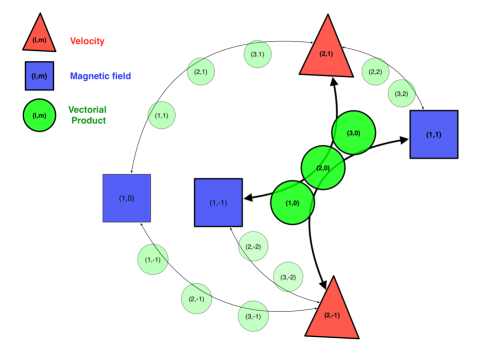
Figure 1.— Schematic coupling between spherical harmonics of $\mathbf{U}$ and $\mathbf{B}$ for the simple test case. The $\mathbf{B}$ modes are represented by blue squares, and the $\mathbf{U}$ modes by red triangles. The black arrows represent the coupling between the modes, the green circles on them represent resulting modes obtained from the coupling via the triangulation rule of the vectorial product $\mathbf{U}\times\mathbf{B}$. The three highlighted green circles in the center correspond to the modes calculated in appendix B.

We stress here that this test has been done for low $m$ and $l$ values. The numerical accuracy of the algorithms calculating the Clebsch-Gordan coefficients (and thus 3j, 6j and 9j Wigner coefficients) is known to decrease with increasing $l$ and $m$. The calculation routines we use are accurate up to values of $l$ of the order of $500$. To do so, we used a multiple precision package to simulate large-precision numbers that are needed to compute the ratios of factorials and binomial coefficients that are involved in the Wigner coefficients calculations. However, the calculation time of the transfer functions $\mathcal{P}$ and $\mathcal{F}$ increases dramatically with $l$ and $m$. For practical reason, when computing fully nonlinear dynamos (see Sect. 4 below), we have chosen to limit the computation of the coupling coefficients to $l_{\rm max}=70$, even if the effective resolution of such simulations reaches $l_{\rm max}=340$. From time to time, we do calculate the transfer terms for high $l$’s to have an indication of how energy is transfered at the smallest scales (see Sect. 4). Nevertheless, the magnetic-energy-carrying scales in the spectrum are dominated by $l\leq 70$ in this case. We thus capture the essential part of the dynamics.

3. Axisymmetric $\alpha\Omega$ dynamo

In this section, we use the spectral method we developed in Sect. 2 on two academic cases. First, we explain how the classical $\Omega$ effect (Moffatt 1978) is represented by our formalism (Sect. 3.1). Then, we calculate the spectral transfers for a mean field $\alpha\Omega$ model (Sect. 3.2).

3.1. Omega effect

The complexity of the two spherical harmonics bases may be confusing when it comes to interpret simple and classical dynamo processes. We thus give hereafter a step-by-step explanation of the $\Omega$-effect in the two vectorial spherical harmonics bases formalism.
We start with a purely dipolar poloidal magnetic field that reads (using Eq. (A9))

$$\mathbf{B}_{p}(r,\theta) = b_{r}(r)\mathbf{R}^{0}_{1}+b_{\theta}(r)\mathbf{S}^{0}_{1}\,.$$ (20)

Then, we want to calculate the effect of a differential rotation that reads

$$\Omega=A+B\cos^{2}\theta\,.$$ (21)

Such differential rotation is usually seen as a “$l=2$” field. Though, it projects on a $l=3$ component when considering the azimuthal component of the velocity $\mathbf{U}_{\varphi}=r\sin\theta\Omega\,\mathbf{e}_{\varphi}$ (see Roberts & Stix (1972)), which reads

$$\mathbf{U}_{\varphi}(r,\theta) = U_{\varphi}(r)\left(A\sin\theta+B\sin\theta\cos^{2}\theta\right)\mathbf{e}_{\varphi}$$ (22)

$$\sim U_{\varphi}(r)\partial_{\theta}Y^{0}_{3}\mathbf{e}_{\varphi}=U_{\varphi}(r)\mathbf{T}^{0}_{3}\,.$$ (23)

In general, Eq. (22) should project both on $\mathbf{T}^{0}_{1}$ and $\mathbf{T}^{0}_{3}$. For the sake of simplicity, we select here a profile of differential rotation that is purely described by a $(l=3,m=0)$ harmonic, which corresponds to $B=-5A$ (Eq. (21)). We simply apply the curl operator (A9) and make use of the coupling relations (A17) to obtain the production of $\mathbf{B}$ in the induction equation,

$$\boldsymbol{\nabla} \times\left(\mathbf{U}_{\varphi}\times\mathbf{B}_{p}\right)=f\left(b_{r},b_{\theta},U_{\varphi}\right)\mathbf{T}^{0}_{2}\,.$$ (24)

We recovered that the action of differential rotation on a purely axisymmetric poloidal field creates a toroidal field $B_{\varphi}\propto\sin\theta\cos\theta$. With our notations, this kind of field will be labeled as a ’$l=2$’ field.

An additional feature of the differential rotation can also be learnt from this little analysis. We immediately remark that for axisymmetric fields, the first Wigner coefficient involved in the coupling between two shells $L_{1}$ and $L_{2}$ is zero if $3+l_{1}+l_{2}$ is odd (equation (A25)), i.e., if $l_{1}$ and $l_{2}$ are of the opposite parity. The shearing effect of differential rotation will then always couple axisymmetric scales of the magnetic field that are of opposite parity, which will be observed in the transfer maps in more complex cases (e.g., Figs 3(b) and 13).

This simple example strikingly highlights how the vectorial product formula (A17) couples together two simple fields. This description of the $\Omega$ effect will guide our analysis in Sects. 3.2 and 4.

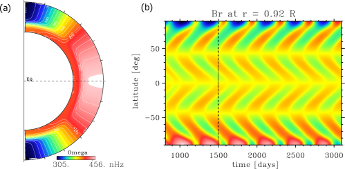
Figure 2.— (a) Solar like differential rotation profile computed from Schou et al. (1998). The tachocline is located near $r=0.7\,R_{\odot}$, and the base of the tachocline rotates at the solar rotation rate $\Omega_{0}=2.6\,10^{-6}\,s^{-1}$. (b) Butterfly diagram in the axisymmetric $\alpha-\Omega$ dynamo (only $B_{r}$ as a function of time and latitude is shown, in the upper convection zone). The vertical black dotted line represent the time at which we display the spectral interactions in Fig. 3.

3.2. Case of a cyclic mean field dynamo

We use the ASH code (Clune et al. 1999; Brun et al. 2004) to simulate an axisymmetric mean field dynamo (Charbonneau 2010; Jouve et al. 2008). To do so, we solve only the induction equation considering uniquely a prescribed differential rotation profile (see also section 3.8 of Jouve et al. 2008, for a similar use of a 3D spherical code to model $\alpha-\Omega$ dynamos).

Our radial domain is defined between $r_{b}=0.6\,R_{\odot}$ and $r_{t}=0.966\,R_{\odot}$. We use a resolution of $N_{r}\times N_{\theta}\times N_{\varphi}=64\times 128\times 256$. We choose a solar differential rotation profile $\Omega_{DR}(r,\theta)=-\partial_{\theta}Z_{DR}/(r^{2}\sin\theta)$ through the toroidal component $Z_{DR}$ of the momentum, which is, in the frame rotating at $\Omega_{0}=2.6\,10^{-6}\,s^{-1}$:

$$Z_{DR}(r,\theta)=Z_{t}(r)\left(A\cos\theta+\frac{B}{3}\cos^{3}\theta+\frac{C}{5}\cos^{5}\theta\right)\,.$$ (25)

From Schou et al. (1998), we take $A=257$ nHz, $B=321$ nHz and $C=529$ nHz. The differential rotation then naturally projects on $\mathbf{U}^{0}_{1}$, $\mathbf{U}^{0}_{3}$ and $\mathbf{U}^{0}_{5}$. The radial profile $Z_{t}(r)$ is chosen such as to simulate a stable region at the base of the domain and is defined by

$$Z_{t}(r)=\bar{\rho}\frac{r^{2}}{2}\left[1+\tanh{\left(\frac{r-4.87\,10^{10}}{2\,10^{9}}\right)}\right]\,.$$ (26)

We initialize our magnetic field with a seed $l=3$ poloidal (antisymmetric and axisymmetric) field.Finally, we add an $\alpha$ effect to the induction equation such that

$$\partial_{t}\mathbf{B}=\mbox{\boldmath$\nabla$}\times\left(\mathbf{U}\times\mathbf{B}+\alpha B_{\varphi}\mathbf{e}_{\varphi}\right)-\mbox{\boldmath$\nabla$}\times\left(\eta\mbox{\boldmath$\nabla$}\times\mathbf{B}\right)\,.$$ (27)

Since we do not take into account in this simple case the feedback of the Lorentz force on the flow via the Navier-Stokes equations, since we only solve the induction equation, we need to quench the $\alpha$ effect. Hence, $\alpha$ is defined by

$$\alpha(r,\theta) = \alpha_{0}\,e^{\left(-\frac{r-0.75\,R_{\odot}}{0.05\,R_{\odot}}\right)^{2}}\,\frac{\cos\theta}{1+(|\mathbf{B}|/B_{q})^{2}}\,.$$ (28)

This is the simplest $\alpha$ that is needed to trigger an oscillating solar-like dynamo (Charbonneau 2010); it is anti-symmetric with respect to the equator. The radial profile of $\alpha$ is localized near the base of the convection zone and the quenching value is given by $B_{q}=10^{3}$ G. We have deliberately chosen an $\alpha$-effect that operates only on the poloidal component of the induction equation, therefore computing an $\alpha\Omega$ mean field dynamo (Moffatt 1978). This $\alpha\Omega$ dynamo exhibits the characteristic butterfly diagram showed in Fig. 2(b) (at $r=0.92\,R_{\odot}$). Although this $\alpha$ profile is ad-hoc and one among the many profiles that were tested in the literature (e.g., Roberts & Stix 1972; Charbonneau & MacGregor 1997; Bonanno et al. 2002; Zhang et al. 2003; Jouve et al. 2008), we chose this form because it easily triggers an oscillatory dynamo and its effect in spectral space can be easily calculated. It is consequently a good choice to illustrate our new spectral method. With the parameters we chose, the cycle period is of the order of $400$ days (see Fig. 2(b)).

The extra $\alpha$ effect adds a new term in the spectral energy equation (16) that can lead to complex formula in spectral space. We rewrite the energy equation

$$\partial_{t}E^{\rm mag}_{L}=\mathcal{D}_{L}+\int_{S}\boldsymbol{\nabla}\times\left(\alpha B_{\varphi}\mathbf{e}_{\varphi}\right)_{L}\cdot\mathbf{B}_{L}\hskip 5.69046pt\mbox{d}{\Omega}$$

$$+\sum_{L_{1},L_{2}}\left\{\mathcal{P}_{L}\left(L_{1},L_{2}\right)+\mathcal{F}_{L}\left(L_{1},L_{2}\right)\right\}\,.$$ (29)

The interested reader may read Appendix A.4 for a complete spectral description of this $\alpha$ effect.

Wherever $|\mathbf{B}|$ is not too large, the quenching part of the $\alpha$ effect is negligible. In that case, the $\alpha$ effect (which restores poloidal field from toroidal field) simply couples a $L$ shell of toroidal field to its neighboring shells of poloidal field, namely $L-1$ and $L+1$. When $|\mathbf{B}|/B_{q}$ becomes large, the $\alpha$ effect is quenched and the poloidal magnetic field stops being restored. When it is sufficiently low, $\alpha$ stops being quenched and the poloidal field grows again. This sets up a simple feedback mechanism and a cycle establishes.

The magnetic energy spectrum is dominated by a $L=2$ component that sets the phase of the total cycle. The various shells energy oscillate with roughly the same period, but are generally out of phase. This phase shift is a natural ingredient that allow the reversal of the overall field polarity (Knobloch et al. 1998; Tobias 2002).

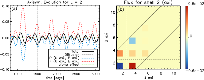
Figure 3.— (a) Evolution of the different terms of equation (29) for the shell $L=2$. Production $\mathcal{P}$ is the dashed blue line, flux $\mathcal{F}$ the dashed red line, diffusion $\mathcal{D}_{1}+\mathcal{D}_{2}$ the dotted black line and the $\alpha$ effect is the dash-dot green line. The black plain line is the total of all the contributions. (b) Flux $\mathcal{F}$ contribution to the $L=2$ shell (see Eq. (29)) at $t=1500$ days (vertical dotted line in panel (a)). The 2D color maps are the $\mathbf{B}^{0}-\mathbf{U}^{0}$ transfer functions (dark red is the maximum value, black the minimum). The oblique black lines represent the boundaries of the triangular selection rule.

We stress here that the magnetic field created in this experiment is of the primary family ($(\mathbf{R}^{0}_{2l+1},\mathbf{S}^{0}_{2l+1})$ and $\mathbf{T}^{0}_{2l}$, see appendix A.7). Our initial magnetic field is a poloidal primary field ($\mathbf{R}^{0}_{3},\mathbf{S}^{0}_{3}$). As a result, the toroidal field created through the $\Omega$-effect is also a primary field ($\mathbf{T}^{0}_{2}$, see section 3.1). Then, our $\alpha$-effect, that creates poloidal field from toroidal field, transforms the primary toroidal field into a primary poloidal field $(\mathbf{R}^{0}_{1,3},\mathbf{S}^{0}_{1,3})$, which is of the same type than our initial magnetic field. Hence, no secondary field can be created in the simulation (which is confirmed by our results), and the $\alpha$-effect can only act on the primary toroidal field to create a primary poloidal field. This is a direct consequence of the well-known separability property of the induction equation between the dipolar and quadrupolar families, when symmetric flows and antisymmetric $\alpha$ effect are chosen (Gubbins & Zhang 1993).

We display in Fig. 3(a) the evolution of the different terms of the magnetic energy equation (29) for $L=2$ at $r=0.92\,R_{\odot}$ during the same time period than the butterfly diagram in Fig. 2(b). The primary toroidal field energy clearly evolves due to the production $\mathcal{P}$ (dashed blue line) and flux $\mathcal{F}$ (dashed red line) terms that account for the effect of differential rotation on the magnetic field (as expected, since there are no other production nor advection terms). The two terms cancel each other out with a small time-lag, their sum combines with the ohmic diffusion (dotted line) to produce oscillations (solid line) of the total $L=2$ energy. Note that the $\alpha$ effect plays no role et $r=0.92\,R_{\odot}$ since it is concentrated at the base of the “convection zone” (equation (28)).

Our new method allows us to characterize how scales interact to produce this behavior. We display in Fig. 3(b) the transfer map for the flux $\mathbf{F}$ term of equation (29) for the $L=2$ shell at its maximum. The differential rotation is composed of the $\mathbf{U}^{0}_{1}$, $\mathbf{U}^{0}_{3}$ and $\mathbf{U}^{0}_{5}$ shells (eq. (25)). The transfer maps during minima (not shown here) are qualitatively opposite, which means that all the couplings between the shells reverse sign during the cycle. This reversal of all shells is a simple, direct consequence of the reversal of the whole magnetic field. At this position, the poloidal magnetic energy (not shown here) evolves because of the ohmic diffusion of the $\alpha$-driven poloidal field at deeper radii. Here, the poloidal magnetic field couples with the differential rotation to transfer energy to the toroidal $L=2$ magnetic shell. The $\mathbf{U}^{0}_{3}-\mathbf{B}^{0}_{1}$ appears to be the dominant interaction that sets the $L=2$ cycle. Interestingly, we will recover this feature in the turbulent (convective) dynamo described in section 4 (see Fig. 13(b).)

This $\alpha\Omega$ dynamo provides a simple example of how our diagnostic may be interpreted in the context of stellar dynamo. Based on how our diagnostic highlights the saturating properties of the solar differential rotation in an $\alpha-\Omega$ case, we now apply it to a turbulent dynamo triggered in a stellar convection zone that also exhibit a solar-like differential rotation profile.

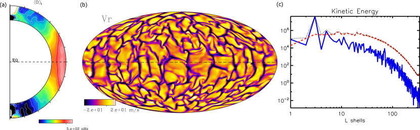
Figure 4.— Progenitor hydrodynamical state. (a) Mean differential rotation profile averaged over 3 months. (b) Time-dependent convective patterns at the top of the convection zone with dark tones representing downflows. (c) Kinetic energy spectra in the middle of the convection zone. The axisymmetric spectra are in plain blue, the non-axisymmetric spectra in dashed red and the total spectra in dotted black.

4. Nonlinear convective dynamo

We use the general method described in Section 2 and validated in Section 3 to study dynamo action in a global (spherical) nonlinear convection zone. Contrary to Section 3, we now solve the full set of MHD equations and do not introduce any $\alpha$ effect. We model a turbulent solar convection zone (Brun et al. 2004; Jouve & Brun 2009; Pinto & Brun 2012) that develops a solar-like differential rotation profile (Fig. 4(a)), with fast equator and slow poles. We display the convective patterns we obtain in Fig. 4(b). We recover the well-known ’banana’-shaped cells at the equator, and more patchy patterns at higher latitudes. Our choice of parameters yields a mildly turbulent state (based on the maximum amplitude of the velocity, the Reynolds number in the middle of the convection zone is of the order of $800$).

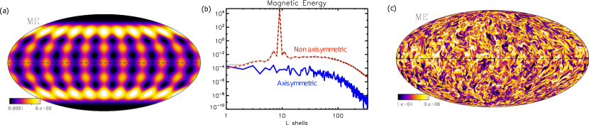
Figure 5.— (a) Initial magnetic energy (the seed poloidal streamfunction is a $l=9,m=5$ spherical harmonic) in cgs, in the middle of the convection zone. (b) Magnetic energy spectra one time step after the introduction of the peaked magnetic field in our turbulent convection zone. The axisymmetric spectra are in plain blue, the non-axisymmetric spectra in dashed red and the total spectra in dotted black. (c) Saturated magnetic energy in cgs, 600 days after the introduction of the seed magnetic field. The color scale is logarithmic.

We display in Fig. 4(c) the kinetic energy spectra in the rotating frame at the center of the convection zone as a function of the shell $L$. We separate the axisymmetric component (the plain blue line) from the non-axisymmetric component (the dashed red line), and the dotted black line is the total spectrum. Notice that two peaks at $L=3,5$ dominate the kinetic energy spectrum. They represent the differential rotation of the azimuthal component of the toroidal velocity (see Sect. 3.1).

We initialize a peaked $(l,m)=(9,5)$ non-axisymmetric magnetic field (Fig. 5(a)) throughout the convection zone by setting:

$$\mathbf{B}=\frac{10\,B_{0}R_{\odot}^{2}}{r^{2}}\left(\frac{R_{b}}{r}\right)^{9}\mathbf{R}_{9}^{5}\,-\frac{B_{0}R_{\odot}^{2}}{r^{2}}\left(\frac{R_{b}}{r}\right)^{9}\mathbf{S}^{5}_{9}.$$ (30)

We set $B_{0}=100$ G so the initial magnetic energy contained in the $L=9$ shell is comparable to the kinetic energy at that scale (see Fig. 5(b)).

The magnetic Prandtl number throughout the convection zone is set to $P_{m}=\frac{\nu}{\eta}=4$, leading to a magnetic Reynolds number of the order of $3200$ at mid-convection zone (based on the maximum amplitude of the velocity). Such a set of parameters triggers a dynamo instability and the growth of magnetic energy (see Fig. 6 in the following).

The initialization we chose allows us to directly see how a significant amount of energy can be transfered to large scales. We also did the same numerical experiment varying the initial conditions. By initializing roughly the same amount of energy distributed over the whole scales, we obtained the same statistical saturated state. Hence, this proves that in this case, the initial scale is forgotten when the dynamo saturates.

The complex interactions between the convective motions and the initially peaked magnetic field lead to the construction of the magnetic energy spectrum. The saturated magnetic energy after 600 days of evolution is displayed on Fig. 5(c) in physical space, in the middle of the convection zone. In the remainder of this section, we characterize how such a state is obtained, and maintained. We distinguish two regimes: the development of the spectrum shape (the kinematic regime, Sect. 4.1), and its saturation and sustainment (the non-linear regime, Sects. 4.2 and 4.3). The results of this section will be summarized in Fig. 14. We recall here that no $\alpha$ effect has been added to the induction equation (5), dynamo action is naturally achieved since convection is 3D and $R_{m}>R_{m}^{\rm crit}$ (Brun et al. 2004).

4.1. Creation of magnetic energy spectrum:
kinematic phase

We plot in Fig. 6 the evolution of the non-axisymmetric magnetic energy spectrum. The initial spectrum is plotted in blue, and the saturated spectrum in red. In addition, we display in Fig. 6 the evolution of the magnetic energy for 6 different $L$ shells. The total energy evolution is also shown (plain thick line). The initial evolution ($t<100$ days) is shown in logarithmic scale The saturation of magnetic energy is reached at $t\sim 300$ days.

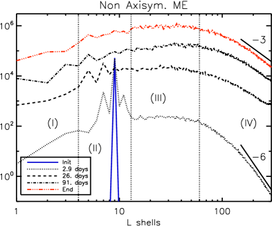
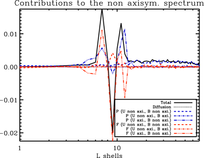
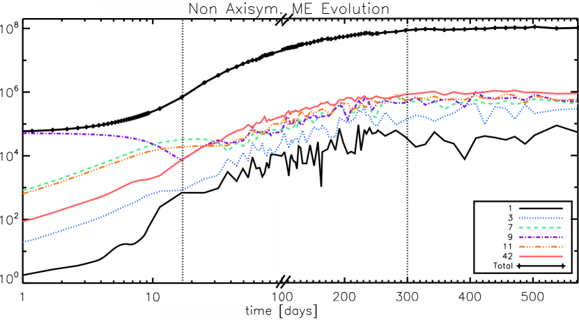
Figure 6.— (a) Evolution of the non-axisymmetric magnetic energy spectra. The initial spectra is blue, the saturated spectrum red. Two slopes ($L^{-6}$ and $L^{-3}$) are given as references for the small scales.(b) Contributions to the non-axisymmetric magnetic energy evolution in the initial phase (dotted line in panel (a)). The total is in plain black, $\mathcal{D}$ in dotted black, $\mathcal{P}$ in blue and $\mathcal{F}$ in red. (c) Evolution of non-axisymmetric energy of shells 1, 3, 7, 9, 11 and 42. Notice the fast early evolution of $E_{7}^{\star}$ and $E_{11}^{\star}$ due to shearing of $\mathbf{B}^{\star}_{9}$ by the differential rotation. The thick plain line is the total non-axisymmetric energy. The abscissa is in log scale between for $t<100$ days, and in linear scale for $t>100$ days. Even though the initial growth is exponential, we chose to represent it in log-log scale to make it appear clearly in the evolution plot.

We also ran another numerical experiment where we artificially suppressed the Lorentz force and the ohmic heating in the momentum and energy equations (i.e., effectively running a kinematic dynamo). On average, the relative difference with the fully non-linear case starts being significantly different (departure of order one) roughly $10$ days after the introduction of the magnetic field (the exact length of the kinematic phase depends on the scale considered). We detail hereafter how the non-axisymmetric (Sect. 4.1.1) and the axisymmetric (Sect. 4.1.2) spectra are created during these first days, which we will refer to as the kinematic phase.

4.1.1 Creation of the non-axisymmetric spectrum

We observe at first that all the $L$ shells gain energy (Fig. 6), excepts the $L=9$ shell which looses energy because it is redistributed throughout the whole domain by the convective flows (Fig. 6). It stops decaying at $t\sim 17$ days. We identify four regions in the non axisymmetric spectrum that exhibit different behaviors. We define the large-scale zone (I) by $1\leq L\leq 4$, the neighborhood zone (II) by $4\leq L\leq 13$, and the plateau zone (III) by $13\leq L\leq 60$. The small-scale zone (IV) ($L\gtrsim 60$) starts at the highest diffusive scale, which is the highest viscous scale $l\sim 60$ based on the first scale at which the local Reynolds number is lower than $1$. It also includes the magnetic dissipative scales ($L\gtrsim 120$). The four zones are separated by the three dotted vertical lines in Fig. 6. In order to understand how the spectrum is built, we display the contributions from the different terms of Eqs. (A32)-(A35) in Fig. 6. Those contributions are taken shortly after the introduction of the magnetic field. They correspond to the spectrum plotted with a dotted line in Fig. 6. We recall that we fully calculate all the coupling terms up to $L=70$.

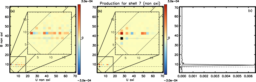
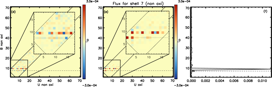
Figure 7.— Production $\mathcal{P}$ and flux $\mathcal{F}$ contributions to the non-axisymmetric shell $L=7$. The 2D color maps are the $\mathbf{B}^{\star}-\mathbf{U}^{\star}$ and $\mathbf{B}^{\star}-\mathbf{U}^{0}$ transfer functions, the 1D plot is the sum of the transfer functions over the $\mathbf{U}$ shells. The horizontal dotted line labels the $\mathbf{B}_{7}$ shell. The oblique black lines represent the boundaries of the triangular selection rule.

The energy transfers around the $L=9$ shell (the neighborhood zone II) are dominated by $\mathbf{U}^{0}-\mathbf{B}^{\star}$ interactions from both the production $\mathcal{P}$ and the flux $\mathcal{F}$ terms. We recall here that both $\mathcal{P}$ and $\mathcal{F}$ represent generic transfer functions, that can either be positive or negative. Dissipation is negligible in zone (II), even for the $L=9$ shell that initially contains the energy. The $L=9$ energy then decreases through the interaction of $\mathbf{B}^{\star}_{9}$ and the differential rotation $\mathbf{U}^{0}_{3}$ that shears the magnetic field (see Sect. 3.1). The energy is preferentially redistributed to $E^{\star}_{11}$ and $E^{\star}_{7}$. For those two shells, the production $\mathcal{P}$ and flux $\mathcal{F}$ terms contribute positively to the creation of the spectrum (Fig. 6). We display in Fig. 7 the detailed contribution of $\mathcal{P}$ and $\mathcal{F}$ to $E^{\star}_{7}$. We only display contributions from $\mathbf{B}^{\star}$ because the axisymmetric magnetic energy is very small initially. The $\mathbf{U}^{\star}-\mathbf{B}^{\star}$ interactions are displayed in panel (a), and the $\mathbf{U}^{0}-\mathbf{B}^{\star}$ interactions in panel (b). We sum over the velocity shells to plot the production term against $\mathbf{B}^{\star}$ in panel (c). We observe that the summed contribution is dominated by $\mathbf{B}^{\star}_{9}-\mathbf{U}^{0}_{3}$ interactions, as expected. Also, we observe that energy is directly transfered from $E_{9}$ to $E_{7}^{*}$, such that the $L=8$ shell is not involved in the transfer. This is true for all the shells in zone (II) and implies that the transfer of energy is non-local, even for shells close to the initial energetic shell.

Due to the triangular selection rule, the $\mathbf{U}^{0}_{3}-\mathbf{B}^{\star}_{9}$ interaction can only act in zone (II). Indeed, $L$ must be strictly greater than $12$ in zones (III-IV) and strictly lower than $6$ in zone (I). $\mathbf{U}^{0}_{3}$ and $\mathbf{B}^{\star}_{9}$ initially dominate respectively the kinetic and magnetic energy spectra. Their interaction was consequently dominant in zone (II), and we expect a different kind of spectral transfers in the other zones. This zone exists because of our choice of initial condition. The very early evolution would have been changed if we had chosen a different initial shell. Though, as stated before, this initial scale is forgotten when the saturated state is reached (Fig. 6).

The dynamics of zones (I), (III) and (IV) are dominated by two effects which competes initially: a direct non-local $\mathbf{B}^{\star}_{9}-\mathbf{U}^{\star}$ transfer of energy, and an effective shearing of neighbor shells by the large scale differential rotation ($\mathbf{B}^{\star}-\mathbf{U}^{0}_{3}$ interactions). These two effect are exemplified in Fig. 8 for $L=42$ (zone III).

Figure 8.— Production $\mathcal{P}$ contribution to the non-axisymmetric shell $L=42$

In the case of the large-scale zone (I) (not shown here), the evolution is dominated by both $\mathcal{P}$ and $\mathcal{F}$. The interactions between $\mathbf{B}^{\star}_{9}$ and $\mathbf{U}^{\star}$ alternate signs depending on the $\mathbf{U}^{\star}$ shell considered. We also stress that the interactions involving other $\mathbf{B}^{\star}$ shells are not negligible. The differential rotation action is completely negligible compared to $\mathbf{U}^{\star}-\mathbf{B}^{\star}$ interactions in zone(I).

In the case of the plateau zone (III), almost a flat profile in the log-log plot is observed in Fig. 6 (hence its name). This plateau is characteristic of convective flows that usually exhibit a broad spectrum between the injection and inertial ranges (Fig. 4(c)). The evolution of the spectrum is dominated only by the $\mathcal{P}_{L}\left(L_{1},L_{2}\right)$ contributions ($\mathcal{F}$ is negligible), and in particular by the coupling between (non-axisymmetric) $\mathbf{U}^{\star}$ and $\mathbf{B}^{\star}$ (Fig. 6). Hence, it is a non-local transfer of magnetic energy that creates the spectrum. All the shells in zone (III) receive energy mainly through this non-local mechanism. As a result, the energy transfer is very sensitive to the kinetic energy contained in the $\mathbf{U}_{L}^{\star}$ shells involved in the coupling. This explains why the magnetic energy spectrum reflects the kinetic energy spectrum in this region.

Although the $\mathbf{U}^{\star}-\mathbf{B}^{\star}$ interactions dominate (Fig. 8), we stress that the $\mathbf{U}^{0}-\mathbf{B}^{\star}$ interactions exhibit a direct cascade pattern. $E^{\star}_{42}$ receives energy from $E^{\star}_{40}$ through $\mathbf{U}^{0}_{3}-\mathbf{B}^{\star}_{40}$ interactions, and gives energy to $E^{\star}_{44}$ through $\mathbf{U}^{0}_{3}-\mathbf{B}^{\star}_{44}$ interactions (see panel (b) in Fig. 8). Even if the triadic interaction involves the large scale velocity $\mathbf{U}^{0}_{3}$, we nonetheless refer this effect as a cascade. The velocity field only acts here as a mediator, and the scales of magnetic field involved in the magnetic energy transfer are at the same scale. It is consequently a cascade when considering the scales of magnetic field.

The energy transfers in zone (IV) (not shown here) are very similar to zone (III). A noticeable difference is that the cascade of energy triggered by the shear of the differential rotation $\mathbf{U}^{0}_{3}$ is much less efficient since the smallest scales hardly feel the large scale rotation profile. Finally, ohmic diffusion acts in the whole zone (IV) and tends to dissipate energy. It has a sufficiently lower amplitude than the non-local transfers so that it does not dictate the spectrum shape initially. It will nevertheless contribute to the saturation process (Sect. 4.2).

4.1.2 Creation of the axisymmetric spectrum

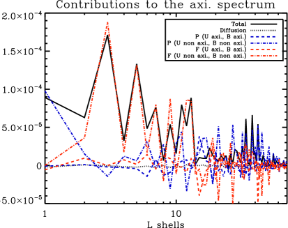
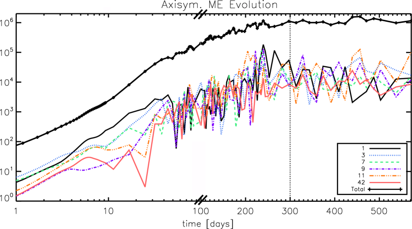
Figure 9.— Same as Fig. 6, for the axisymmetric part of the spectrum. In panel (a), the initial spectrum is zero.

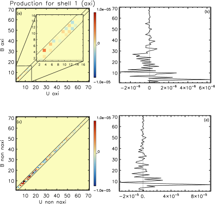
Figure 10.— Production $\mathcal{P}$ for the axisymmetric shell $L=1$ during the initial state. Both $\mathbf{U}^{0}-\mathbf{B}^{0}$ and $\mathbf{U}^{\star}-\mathbf{B}^{\star}$ couplings are shown.

We now characterize the creation of the axisymmetric spectrum. We display in Fig. 9 the evolution of the axisymmetric component of the magnetic energy. We recall that since we initialize the dynamo with a purely non-axisymmetric field, the initial axisymmetric spectrum is null. After one time-step, the axisymmetric magnetic energy is orders of magnitude lower than the non-axisymmetric spectrum (Fig. 5(b) The global shape of the axisymmetric spectrum is created very rapidly, all the shells gain energy at about the same rate until they saturate. The initial exponential growth rate is the same for both the axisymmetric and non-axisymmetric spectrum is approximately $0.6$ days^-1 (which corresponds to a time-scale approximately $17$ times lower than the convective turn-over time). This can also be observed on Fig. 9, where we plot the evolution of few shells against time. They all gain energy at about the same rate initially, and then slowly tend to a saturated state. The axisymmetric shells considered have comparable energy since the spectrum is essentially flat at scales $L\leq 30$ (Fig. 9), which was not the case for the non-axisymmetric spectrum (Fig. 6). We observe in Fig. 9 that the flux term $\mathcal{F}$ plays a major role between $L=2$ and $L=13$. This means that the creation of the spectrum is dominated by the radial interactions at those scales. The two flux curves exhibit a sawtooth pattern that is again reminiscent from the differential rotation energy shells (see Sects. 3.1 and 4.1.1). At higher $L$, the evolution of the spectrum is the result of a complex interplay between the production and flux terms.

More interesting, the dipole ($L=1$) evolution is dominated by the production term through the interaction between the non axisymmetric magnetic field and velocity field. We display the detailed transfers maps for this scale on Fig. 10. We observe that the large scale magnetic field is mainly created by the interplay between $\mathbf{B}_{7}^{\star}$ and $\mathbf{U}^{\star}_{6-8}$. The transfers involving $\mathbf{B}_{9}^{\star}$ (where the energy is originally mainly contained) act negatively and do not dominate the transfer of magnetic energy. This is consistent with the fact that the whole axisymmetric spectrum shape is rapidly created and only gains energy globally afterwards. It does not depend on the scale at which we initially put the non-axisymmetric magnetic energy. Since the energy is not transfered directly from the initial reservoir of energy $E_{9}^{\star}$, we already see preferred transfers towards the large scale dipole involving $\mathbf{B}^{\star}_{7}$, which is one of the highest energy scale of the non-axisymmetric spectrum at this time. This effect shall be confirmed during the saturation phase (Sect. 4.3). The creation of the axisymmetric magnetic energy spectrum seems to depend essentially on the initial hydrodynamic convective spectrum (as expected in such kinematic phase).

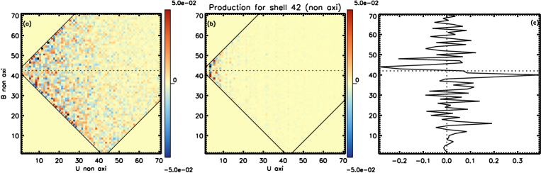
Figure 11.— Production $\mathcal{P}$ contribution to the non-axisymmetric shell $L=42$ during the saturation phase. Interactions between $\mathbf{B}^{0}$ and $\mathbf{U}^{\star}$ are negligible.

4.2. Non-linear saturation of the smallest scales

Following Sect. 4.1, we now detail the saturation and sustainment of the magnetic energy spectrum at small scales. By $500$ days the axisymmetric and non-axisymmetric spectra are saturated (Figs. 9 and 6).

The flux $\mathcal{F}$ contribution is likely to never be null at the largest scales since it represents the flux of magnetic energy through the horizontal surface at the middle of the turbulent convection zone. In order to saturate the magnetic energy (i.e., to get $dE_{L}^{\rm mag}/dt=0$), $\mathcal{D}$ and/or $\mathcal{P}$ have to compensate $\mathcal{F}$. In the first three zones, diffusion is negligible. Hence, $\mathcal{P}$ naturally tends to cancel $\mathcal{F}$ out in those zones (see Sect. 3.2 for a simple version of this cancellation effect). The cancellation effect is such that $\mathcal{F}(\mathbf{U}^{\star},\mathbf{B}^{\star})$ tends to cancel $\mathcal{P}(\mathbf{U}^{\star},\mathbf{B}^{\star})$ out. This is also the case for $\mathcal{F}(\mathbf{U}^{0},\mathbf{B}^{\star})$, $\mathcal{F}(\mathbf{U}^{\star},\mathbf{B}^{0}$), and $\mathcal{F}(\mathbf{U}^{0},\mathbf{B}^{0})$.

In spite of the cancellation of the different contributions, characteristic patterns can still be identified. The more distinctive pattern we identified in Sect. 4.1 was the direct cascade of magnetic energy in zone (III). It turns out that we still observe it and that it slightly dominates the transfer terms during the saturation phase. We display on Fig. 11 the production contribution to the non-axisymmetric magnetic energy evolution $600$ days after the magnetic field introduction. We recover the direct cascade of energy in the production contribution, that was already present on Fig. 8. This direct cascade of energy is associated with an inverse cascade of energy carried by the flux contribution, which opposes the production term during the saturation phase. Both cascades are of the same order of magnitude and tend to cancel each other out. They are associated with the axisymmetric component $\mathbf{U}^{0}_{3}$ (the differential rotation), and the non-axisymmetric components of $\mathbf{B}$. The contributions of non-axisymmetric components of $\mathbf{U}$ involve more shells, but their net effect is a bit lower than the shear from differential rotation (panel (a) on Fig 11). On this panel, no particular global pattern can be identified.

The transfers of magnetic energy appear to be very interesting in zone (IV) where diffusion acts significantly. In order to saturate, $\mathcal{P}$ and $\mathcal{F}$ have to combine to cancel $\mathcal{D}$. For the non-axisymmetric spectrum, it is the production term that dominates over the flux term to compensate diffusion. In addition, the production term in zone (IV) exhibits a very particular generalized cascade shape. This cascade could not be identified during the early evolution for it was dominated by the non-local transfer from $\mathbf{B}^{\star}_{9}$. We display on Fig. 12 (panel a) the $\mathbf{U}^{\star}-\mathbf{B}^{\star}$ production map towards $E^{\star}_{152}$. The other interactions are negligible. We observe that the map is dominated by positive contribution (red) under the horizontal dashed line ($L=152$), and by negative contribution (blue) above. This is confirmed by the plot in panel b where the transfers have been summed over the velocity shells. This cascade is of different kind than the one observed in zone (III) (Fig. 11). Here, no clear velocity shell dominates the transfer map (panel a on Fig. 12). It is a generalized cascade that results from the coupling between many magnetic shells (around $L=152$) and all the largest velocity scales. Hence, the velocity scales involved in the cascade are not local compared to the magnetic field scale considered.

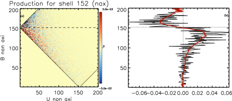
Figure 12.— Production $\mathcal{P}$ contribution to the non-axisymmetric shell $L=152$ during the saturation phase. The red line is the smoothed contribution, that exhibits the characteristic S-shape of the generalized cascade.

Trying to simplify the complex 2D transfer maps, one may isolate the main contributing couplings to the different evolution terms. Doing so at all times for the non-axisymmetric spectrum at small scales, we find that the percentage of couplings that account for $90$% of the contributing terms typically varies from nearly $1$ to $70$% of the calculated couples. As a result, we demonstrate here that the complex dynamo process occurring in a 3D turbulent convection zone involves many modes that interact though non-trivial triadic interactions. Then, the dynamics of the smallest scales can hardly be reduced to the evolution of a small set of modes.

Finally, the analysis of the axisymmetric $\alpha\Omega$ dynamo in Sect. 3.2 shed light on the importance of the families of symmetry (with respect to the equator) of the fields. The instantaneous convective motions do not exhibit any particular symmetry at any scale and the kinetic energy spectrum is a mixture of both primary and secondary velocities. The differential rotation is the only velocity feature that has a clear symmetry (secondary family, see Sect. 3.1) and that has a large influence on the magnetic energy spectrum. It is involved in the magnetic energy cascade in zone (III), and shears both primary and secondary magnetic fields to cascade primary and secondary magnetic energy. Thus, it does not select a particular symmetry. Indeed, the ratio of primary (antisymmetric) to secondary (symmetric) magnetic energy varies with time for all shells and does not settle even during the saturation phase. The presence of complex flows, often breaking the equatorial symmetry, yields a strong coupling of both dynamo families (as in the Sun, see DeRosa et al. (2012)), contrary to simpler mean field dynamo models (see Sect. 3).

4.3. Sustainment of the mean large scale magnetic field

Given their key role in setting the overall magnetic polarity in the Sun (DeRosa et al. 2012), we now detail the main contributions to the saturation and sustainment of the large scale axisymmetric dipole $(l=1,m=0)$ and quadrupole $(l=2,m=0)$ fields.

At the late phase of the simulation the large-scale axisymmetric spectrum is fully saturated (Fig. 9). The saturation is obtained thanks to the compensation of the production and flux terms, similarly to the saturation of the mid-scales (see previous section). The large-scale dipole $(l=1,m=0)$ saturation process differs significantly from its creation. We display in Fig. 13 the production maps for the axisymmetric dipole and quadrupole averaged over $150$ days during the saturated state. The transfers maps of $\mathcal{F}$ (not shown here) are exactly opposite to the maps (a) and (c) for $\mathcal{P}$. We see that both the axisymmetric and non-axisymmetric fields significantly contribute to the saturation and sustainment of the large scale dipole. In particular, two main contributors emerge. First (panel a), the coupling of the differential rotation $\mathbf{U}^{0}_{3}$ with the large scale $\mathbf{B}^{0}_{4}$ field dominates the axisymmetric contributions. This effect is more likely to represent the shearing of the large scale poloidal multipole $\mathbf{B}^{0}_{p}$ by the large-scale toroidal differential rotation.

Second, the non-axisymmetric contributions (panel c) are at least equally important for the saturation of the dipole. In particular, the interaction $\mathbf{U}^{\star}_{23}-\mathbf{B}^{\star}_{23}$ dominates the non-axisymmetric contributions. Thus, is it a non-local interaction that saturates the large-scale magnetic dipole. Furthermore, $\mathbf{B}^{\star}_{23}$ is one of the most energetic shells of the magnetic energy spectrum (Fig. 6). This directly points out the importance of the mid-scale part of both the kinetic and magnetic energy spectra for the saturation level of the large-scale magnetic dipole.

We can remark here that the major contributions of $\mathcal{P}$ for the saturation of the dipole are all positive. They are balanced by negative contributions from $\mathcal{F}$. Consequently, if the differential rotation was more efficient, or if the $\mathbf{U}^{\star}_{23}-\mathbf{B}^{\star}_{23}$ interaction possessed more energy, the saturation level of the large scale dipole would be much higher.

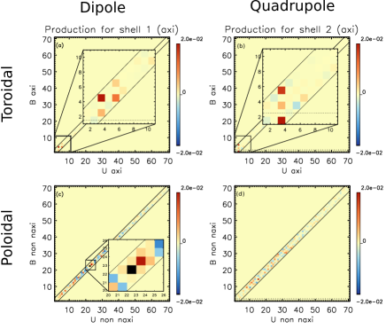
Figure 13.— Saturation of the large scale axisymmetric dipole (panels a and c, production $\mathcal{P}$ for $E^{0}_{1}$) and quadrupole (panels b and d, production $\mathcal{P}$ for $E^{0}_{2}$). The interaction maps are time averaged over a period of $\sim 150$ days. Both $\mathbf{U}^{0}-\mathbf{B}^{0}$ and $\mathbf{U}^{\star}-\mathbf{B}^{\star}$ couplings are shown.

Since our magnetic Prandtl number is $4$, the peak of the kinetic and magnetic energy spectra are likely to be shifted. At saturation, the couplings are nonetheless dominated by the peak of the magnetic energy spectrum that occurs at smaller scale than the peak of the kinetic energy spectrum. Changing the magnetic Prandtl number will cause the separation of the peaks to change. If the peaks separate more, our results suggest that the saturating interaction will involve smaller scales velocity and magnetic fields. The velocity field involved is likely to be less energetic, which could trigger a smaller saturating interaction, and in turn a lower energy state for the large scale dipole. If the peaks are closer (or eventually switch), the picture becomes more complicated and we cannot predict if the saturating interaction will remain fixed by the peak of the magnetic energy spectrum. The exploration of this parameter space is left for future work.

The large scale quadrupole also saturates thanks to both the axisymmetric and non-axisymmetric fields (panels b and d). The axisymmetric contributions (panel b) are very similar to the dipole case and are dominated by the differential rotation. The differential rotation shears both $\mathbf{B}^{0}_{1}$ and $\mathbf{B}^{0}_{5}$, which is opposed by the flux term to saturate the quadrupole. Again, this effect accounts for the saturation of the toroidal quadrupolar field. Hence, the saturated level of the poloidal dipolar field (panel c) plays a major role for the saturation of the toroidal quadrupolar field.

The poloidal quadrupolar field is then saturated through the non-axisymmetric interactions (panel d). The contribution are again very non-local, though in this case no particular scale dominates the saturation process. Hence, we may expect that the saturation process of the axisymmetric quadrupole will have a very different dependency on the magnetic Prandtl number than the axisymmetric dipole.

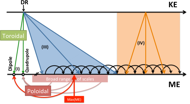
Figure 14.— Saturating interactions of the non-linear convective dynamo summarizing the results of section 4. KE and ME stand for Kinetic and Magnetic Energy and DR for Differential Rotation.

5. Conclusions and Perspectives

In this paper we developed and validated a new spectral analysis method suited for spherical objects. Using two vectorial spherical harmonics basis, we were able to calculate transfer functions of magnetic energy in spectral space. We can calculate the coupling coefficients up to $l\sim 500$. For the first time in such studies, the complete $2$D transfers maps have been calculated to characterize the full triadic interactions.

After a quick numerical validation, we first applied our method to a simplified $\alpha\Omega$ dynamo case. Such axisymmetric models are very well known to trigger cyclic dynamos (Charbonneau 2010) with our choice of a symmetric (with respect to equator) velocity field and an antisymmetric $\alpha$ effect. The clear separation between the dipolar and quadrupolar families was illustrated thanks to our new diagnostic. The production (i.e., on a spherical surface) and a flux (i.e., through a spherical surface) contributions were shown to quasi-cancel each other out for all shells.

Our method was then successfully applied to a 3D turbulent convective dynamo case. We initialize a highly non-axisymmetric magnetic field and let the dynamo develop a turbulent spectrum of magnetic energy. We distinguished the kinematic phase with exponential growth of the magnetic energy spectrum, and the non-linearly saturated phase. The first phase is dominated by both a non-local transfer of energy from the initial scale of magnetic energy, coupled with the convective scales, towards all the other magnetic scales, and the shearing by the large scale differential rotation. A large part of the magnetic energy spectrum is then dictated by the kinetic energy spectrum developed by the convection.

The saturation phase is more subtle and greatly depends on the considered scale in the spectrum. The saturating interactions for the different spectral scales are illustrated in Fig. 14, and summarized hereafter.

Our new method allowed us to distinguish two clear cascades of magnetic energy at the smallest scales of our simulation, for $13\leq L\leq 60$ and $L>60$ (highest $L$’s). In the former case, the differential rotation profile mediates the cascade by shearing the magnetic field. It results in an efficient cascade of magnetic energy.

The latter cascade is also direct and involves all the highest velocity scales (the large scale differential rotation does not dominate in this case). It is a generalized cascade over a large range of magnetic scales. The velocity scales involved in the cascade are not local with respect to the magnetic scales. As consequence, we cannot predict if this generalized cascade would hold at the lowest scales in the case of a real convective dynamo where scale separation is much higher. Besides, the saturation also involve non-local coupling that can eventually be of the order of the sheared cascade for the intermediate scales. We proved in that case that the transfers cannot be reduced to a limited set of modes.

The saturation of the large scale axisymmetric dipole and quadrupole appear to be radically different than the small-scale saturation. The toroidal components are mainly saturated by the balance of the shearing effect of the differential rotation on the large scale poloidal fields, and the flux transfer through the spherical shell due to the effect of the differential rotation. The poloidal components are mainly saturated by non-local non-axisymmetric interactions. The dipole is saturated by the scale of maximum (highest) magnetic energy, and the quadrupole saturation is not dominated by any particular scale. These two observations point to the two main dependencies of the saturating interactions for the large-scale fields. First, the rotation rate of the star (which is linked to the saturating interaction through the differential rotation) can determine the ability of the dynamo to build wreaths (Brown et al. 2010), and/or to be in a strong or weak regime (Christensen & Aubert 2006; Featherstone et al. 2009; Simitev & Busse 2009). Second, the magnetic Prandtl number $P_{m}=\nu/\eta$ determines the postion of the peak of magnetic energy and then affects the saturating interaction (e.g., see Schekochihin et al. 2004). We will explore in detail how the saturating interactions depend on those two effects in future work.

Finally, it is worth comparing theses results with previous related work of Livermore et al. (2010). When using forced helical flows and allowing the dynamo field to back-react on the flow, they found that the saturation of the large scale poloidal dipole was dominated by non-local interaction with a particular magnetic scale ($l=10,m=10$ in their case). They showed that magnetic energy was transfered to this scale by the large-scale toroidal magnetic field. In our case, the large-scale dipole is also saturated due to non-local interactions. Though, the flow we consider is significantly different because (i) it is obtained from the convective instability and (ii) its spectrum is dominated by the large-scale differential rotation that develops self-consistently. Hence, the dynamo process is different and we find that the toroidal large-scale field is saturated by the effect of the large scale differential rotation, and the large-scale poloidal dipole by the non-local transfer of energy from the magnetic scale of maximal energy.

Our results also suggest that no significant large-scale magnetic field is growing over dissipative time scales in our simulation (the ohmic dissipation time scale for the axisymmetric dipole is typically of the order of $\tau_{\eta}\sim 700$ days in the simulation). Again, the fast saturation of the dynamo (less than $300$ days) may not hold for lower magnetic Prandtl number dynamos.

We developed a diagnostic on the magnetic energy that is an invariant of ideal MHD. In the case of non-ideal MHD, the existence of the selective decay (Taylor 1974; Matthaeus & Montgomery 1980; Mininni & Montgomery 2006) introduces a decoupling between, e.g., the evolution time scales of the magnetic (or total) energy (fast) and the magnetic helicity (slow). As mentioned before, we were interested, in this work, in fast phenomena compared to the ohmic diffusion time. For such processes, the ideal invariants of MHD are still the appropriate quantities to interpret the scales interactions. The dynamo saturation is necessarily achieved through a modification of the kinetic energy spectrum. As mentioned before, the case we studied in this paper is in the weak branch of the dynamo (i.e., the large scale poloidal magnetic field does not dominate the magnetic energy spectrum Christensen & Aubert 2006; Simitev & Busse 2009; Gastine et al. 2012). The detailed modification of the kinetic energy spectrum implied by the saturation of the dynamo process will be discussed for both the strong and weak branches in a future work. Although the magnetic energy is the relevant quantity to characterize nearly kinematic dynamos (where the Lorentz force plays little role), a diagnostic on kinetic energy would be highly valuable for non-linearly saturated dynamos. On top of that, the detailed spectral transfers of magnetic helicity are also mandatory to fully address the complexity of the dynamo process. Evolution equations of kinetic energy, magnetic helicity and cross helicity in the framework introduced in this paper are under development and will be published in a forthcoming paper.

Finally, those diagnostics may also prove very useful for non-dynamo transfers related MHD phenomena. For example, spectral analysis applied to the relaxation and the stability of low-l fossil field (see Braithwaite & Nordlund 2006; Brun 2007; Zahn et al. 2007; Duez & Mathis 2010; Duez et al. 2010) will be studied in a future publication.

Appendix A Definition and properties of Vectorial Spherical Harmonics

A.1. Classical vectorial spherical harmonics basis

A.1.1 Definitions

We define from Rieutord (1987); Mathis & Zahn (2005):

$$\left\{\begin{array}[]{lcl}\mathbf{R}^{m}_{l}(\theta,\varphi)&=&Y_{l}^{m}(\theta,\varphi)\mathbf{e}_{r}\\ \mathbf{S}^{m}_{l}(\theta,\varphi)&=&\boldsymbol{\nabla}_{\perp}Y_{l}^{m}=\partial_{\theta}Y_{l}^{m}\mathbf{e}_{\theta}+\frac{1}{\sin{\theta}}\partial_{\varphi}Y_{l}^{m}\mathbf{e}_{\varphi}\\ \mathbf{T}^{m}_{l}(\theta,\varphi)&=&\boldsymbol{\nabla}_{\perp}\times\mathbf{R}^{m}_{l}=\frac{1}{\sin{\theta}}\partial_{\varphi}Y_{l}^{m}\mathbf{e}_{\theta}-\partial_{\theta}Y_{l}^{m}\mathbf{e}_{\varphi}\end{array}\right.,$$ (A1)

where $(\mathbf{e}_{r},\mathbf{e}_{\theta},\mathbf{e}_{\varphi})$ defines the spherical basis and $Y^{m}_{l}$ are the Laplace spherical harmonics defined by

$$Y_{l}^{m}(\theta,\varphi)=(-1)^{\frac{m+|m|}{2}}\sqrt{\frac{(2l+1)}{4\pi}\frac{(l-|m|)!}{(l+|m|)!}}P^{|m|}_{l}(\cos\theta)e^{im\varphi}\,$$ (A2)

where $P^{m}_{l}$ are the associated Legendre polynomials. The basis (A1) have the following properties :

$$\int_{S}\mathbf{R}^{m_{1}}_{l_{1}}\cdot\left(\mathbf{R}^{m_{2}}_{l_{2}}\right)^{cc}\hskip 5.69046pt\mbox{d}{\Omega} = \delta_{l_{1},l_{2}}\delta_{m_{1},m_{2}},$$ (A3)

$$\int_{S}\mathbf{S}^{m_{1}}_{l_{1}}\cdot\left(\mathbf{S}^{m_{2}}_{l_{2}}\right)^{cc}\hskip 5.69046pt\mbox{d}{\Omega} = \int_{S}\mathbf{T}^{m_{1}}_{l_{1}}\cdot\left(\mathbf{T}^{m_{2}}_{l_{2}}\right)^{cc}\hskip 5.69046pt\mbox{d}{\Omega}=l_{1}(l_{1}+1)\delta_{l_{1},l_{2}}\delta_{m_{1},m_{2}},$$ (A4)

where $S$ is a spherical surface, $\hskip 5.69046pt\mbox{d}{\Omega}=\sin\theta\mbox{d}\theta\mbox{d}\varphi$ the solid angle, $cc$ means complex conjugate and $\delta$ is the Kronecker symbol. We also have:

$$(\mathbf{S}^{m}_{l})^{cc}=(-1)^{m}\mathbf{S}^{-m}_{l}\,,$$ (A5)

and all the other scalar cross products are $0$. We remind the reader that the poloidal fields are described by their projection on $(\mathbf{R}^{m}_{l},\mathbf{S}^{m}_{l})$, and the toroidal fields by their projection on $\mathbf{T}^{m}_{l}$.

A.1.2 Scalar fields

Defining $\psi(r,\theta,\varphi)=\sum_{l=1}^{\infty}\sum_{m=-l}^{l}\left\{\psi_{m}^{l}(r)Y_{l}^{m}(\theta,\varphi)\right\}$, we get:

$$\boldsymbol{\nabla}\psi = \sum_{l=1}^{\infty}\sum_{m=-l}^{l}\left\{\partial_{r}\psi_{m}^{l}\mathbf{R}^{m}_{l}+\frac{\psi_{m}^{l}}{r}\mathbf{S}^{m}_{l}\right\},$$ (A6)

$$\boldsymbol{\nabla}\cdot\boldsymbol{\nabla}\psi = \sum_{l=1}^{\infty}\sum_{m=-l}^{l}\Delta_{l}\psi_{m}^{l}Y_{l}^{m}$$ (A7)

where $\Delta_{l}=\partial^{2}_{rr}+\frac{2}{r}\partial_{r}-\frac{l(l+1)}{r^{2}}$.

A.1.3 Vectorial fields

For a vector $\mathbf{X}(r,\theta,\varphi)=\sum_{l=1}^{\infty}\sum_{m=-l}^{l}\left\{\mathcal{A}^{l}_{m}(r)\mathbf{R}^{m}_{l}+\mathcal{B}^{l}_{m}(r)\mathbf{S}^{m}_{l}+\mathcal{C}^{l}_{m}(r)\mathbf{T}^{m}_{l}\right\}$, we obtain:

$$\boldsymbol{\nabla}\cdot\mathbf{X} = \sum_{l=1}^{\infty}\sum_{m=-l}^{l}\left\{\left[\frac{1}{r^{2}}\partial_{r}(r^{2}\mathcal{A}^{l}_{m})-l(l+1)\frac{\mathcal{B}^{l}_{m}}{r}\right]Y_{l}^{m}\right\},$$ (A8)

$$\boldsymbol{\nabla}\times\mathbf{X} = \sum_{l=1}^{\infty}\sum_{m=-l}^{l}\left\{\left[l(l+1)\frac{\mathcal{C}^{l}_{m}}{r}\right]\mathbf{R}^{m}_{l}+\left[\frac{1}{r}\partial_{r}(r\,\mathcal{C}^{l}_{m})\right]\mathbf{S}^{m}_{l}+\left[\frac{\mathcal{A}^{l}_{m}}{r}-\frac{1}{r}\partial_{r}(r\,\mathcal{B}^{l}_{m})\right]\mathbf{T}^{m}_{l}\right\},$$ (A9)

$$\nabla^{2}\mathbf{X} = \sum_{l=1}^{\infty}\sum_{m=-l}^{l}\left\{\left[\Delta_{l}\mathcal{A}^{l}_{m}-\frac{2}{r^{2}}(\mathcal{A}^{l}_{m}-l(l+1)\mathcal{B}^{l}_{m})\right]\mathbf{R}^{m}_{l}\right.$$ (A10)

$$+ \left.\left[\Delta_{l}\mathcal{B}^{l}_{m}+2\frac{\mathcal{A}^{l}_{m}}{r^{2}}\right]\mathbf{S}^{m}_{l}+\left[\Delta_{l}\,\mathcal{C}^{l}_{m}\right]\mathbf{T}^{m}_{l}\right\}\,.$$

A.1.4 Recurrence relations

In addition to the expression of the different operators, we also give here two useful coupling relations between spherical harmonics. First, according to Varshalovich et al. (1988), the coupling between $\cos{\theta}$ and the spherical harmonic $Y_{l}^{m}$ is given by

$$\cos{\theta}\,Y_{l}^{m}=\sqrt{\frac{\left(l-m+1\right)\left(l+m+1\right)}{\left(2l+1\right)\left(2l+3\right)}}Y^{m}_{l+1}+\sqrt{\frac{\left(l-m\right)\left(l+m\right)}{\left(2l-1\right)\left(2l+1\right)}}Y^{m}_{l-1}\,.$$ (A11)

Then, one easily deduces the following properties:

$$\cos{\theta}\,\mathbf{S}^{m}_{l} = \frac{l}{l+1}\sqrt{\frac{\left(l-m+1\right)\left(l+m+1\right)}{\left(2l+1\right)\left(2l+3\right)}}\mathbf{S}^{m}_{l+1}+\frac{l+1}{l}\sqrt{\frac{\left(l-m\right)\left(l+m\right)}{\left(2l-1\right)\left(2l+1\right)}}\mathbf{S}^{m}_{l-1}$$ (A12)

$$- \frac{im}{l\left(l+1\right)}\mathbf{T}^{m}_{l}\,,$$

$$\cos{\theta}\,\mathbf{T}^{m}_{l} = \frac{l}{l+1}\sqrt{\frac{\left(l-m+1\right)\left(l+m+1\right)}{\left(2l+1\right)\left(2l+3\right)}}\mathbf{T}^{m}_{l+1}+\frac{l+1}{l}\sqrt{\frac{\left(l-m\right)\left(l+m\right)}{\left(2l-1\right)\left(2l+1\right)}}\mathbf{T}^{m}_{l-1}$$ (A13)

$$+ \frac{im}{l\left(l+1\right)}\mathbf{S}^{m}_{l}\,.$$

A.2. An alternative vectorial basis

A.2.1 Definitions

The vectorial spherical harmonics basis defined in appendix A.1 is very efficient to calculate scalar products or linear differential operator on vectors. Nevertheless, it is quite hard to use it to express vectorial products. Instead we define the following basis (e.g., see Varshalovich et al. (1988)):

$$\mathbf{Y}_{l,l+\nu}^{\hskip 2.84544ptm}(\theta,\varphi)=\sum_{\mu=-1}^{1}\left\{(-1)^{l-m}\sqrt{2l+1}\left(\begin{array}[]{ccc}l&l+\nu&1\\ m&\mu-m&-\mu\end{array}\right)Y_{l+\nu}^{m-\mu}\mathbf{e}_{\mu}\right\},$$ (A14)

where $(\dots)$ is the $3$-j Wigner coefficient linked to Clebsch-Gordan coefficients, and the vectors $\mathbf{e}_{\mu}$ are

$$\left\{\begin{array}[]{lcl}\mathbf{e}_{-1}&=&\frac{1}{\sqrt{2}}\left(\mathbf{e}_{x}-i\mathbf{e}_{y}\right)\\ \mathbf{e}_{0}&=&\mathbf{e}_{z}\\ \mathbf{e}_{1}&=&-\frac{1}{\sqrt{2}}\left(\mathbf{e}_{x}+i\mathbf{e}_{y}\right)\end{array}\right.,$$ (A15)

where $(\mathbf{e}_{x},\mathbf{e}_{y},\mathbf{e}_{z})$ defines the cartesian basis. Note that the equivalent of the conjugation rule (A5) is then

$$\left(\mathbf{Y}^{m}_{l,l+\nu}\right)^{cc}=\left(-1\right)^{m+\delta_{0\nu}}\mathbf{Y}^{-m}_{l,l+\nu}\,.$$ (A16)

Again, we recall that the poloidal fields are described by their projection on $(\mathbf{Y}^{m}_{l,l+1},\mathbf{Y}^{m}_{l,l-1})$ ($\nu\in\left\{-1;1\right\}$), and the toroidal fields are described by their projection on $\mathbf{Y}^{m}_{l,l}$ ($\nu=0$).

A.2.2 Vectorial product

We decompose a vector $\mathbf{X}$ on this basis in the following way:

$$\mathbf{X}(r,\theta,\varphi)=\sum_{l=1}^{\infty}\sum_{m=-l}^{l}\sum_{\nu=-1}^{1}X_{l,l+\nu}^{\hskip 2.84544ptm}(r)\mathbf{Y}_{l,l+\nu}^{\hskip 2.84544ptm}.$$

Evaluating the vectorial product of two vectors $\mathbf{X}_{12}=\mathbf{X}_{1}\times\mathbf{X}_{2}$, one gets:

$$X_{12;l_{12},l_{12}+\nu_{12}}^{\hskip 2.84544ptm_{12}}=\sum_{\begin{subarray}{c}l_{1},l_{2}=1\\ l_{12}\geq|l_{1}-l_{2}|\\ l_{12}\leq l_{1}+l_{2}\end{subarray}}^{\infty}\sum_{\begin{subarray}{c}m_{1}=-l_{1}\\ m_{2}=-l_{2}\\ m_{1}+m_{2}=m_{12}\end{subarray}}^{l_{1},l_{2}}\sum_{\nu_{1},\nu_{2}}X_{1;l_{1},l_{1}+\nu_{1}}^{\hskip 2.84544ptm_{1}}X_{2;l_{2},l_{2}+\nu_{2}}^{\hskip 2.84544ptm_{2}}\mathcal{J}^{l_{12},m_{12},\nu_{12}}_{l_{1},m_{1},\nu_{1},l_{2},m_{2},\nu_{2}},$$ (A17)

where

$$\mathcal{J}^{l,m_{1}+m_{2},\nu}_{l_{1},m_{1},\nu_{1},l_{2},m_{2},\nu_{2}}=i(-1)^{\nu_{1}-\nu_{2}+(m_{1}+m_{2})}$$

$$\sqrt{\frac{3}{2\pi}(2l_{1}+1)(2l_{1}+2\nu_{1}+1)(2l_{2}+1)(2l_{2}+2\nu_{2}+1)(2l+1)(2l+2\nu+1)}$$

$$\left\{\begin{array}[]{ccc}l_{1}&l_{2}&l\\ l_{1}+\nu_{1}&l_{2}+\nu_{2}&l+\nu\\ 1&1&1\end{array}\right\}\left(\begin{array}[]{ccc}l_{1}&l_{2}&l\\ m_{1}&m_{2}&-(m_{1}+m_{2})\end{array}\right)\left(\begin{array}[]{ccc}l_{1}+\nu_{1}&l_{2}+\nu_{2}&l+\nu\\ 0&0&0\end{array}\right),$$ (A25)

with $\{\cdots\}$ being the $9$-j Wigner coefficient.

A.3. Basis change relations

For a vector $\mathbf{X}$ decomposed in the following manner:

$$\mathbf{X} = \sum_{l=1}^{\infty}\sum_{m=-l}^{l}\left\{\mathcal{A}^{l}_{m}\mathbf{R}^{m}_{l}+\mathcal{B}^{l}_{m}\mathbf{S}^{m}_{l}+\mathcal{C}^{l}_{m}\mathbf{T}^{m}_{l}\right\}$$

$$= \sum_{l=1}^{\infty}\sum_{m=-l}^{l}\sum_{\nu=-1}^{1}\left\{X_{l,l+\nu}^{\hskip 2.84544ptm}\mathbf{Y}_{l,l+\nu}^{\hskip 2.84544ptm}\right\},$$

we have the two following relations to change from one basis to the other:

$$\left\{\begin{array}[]{lcl}\mathcal{A}^{l}_{m}&=&\frac{1}{\sqrt{2l+1}}\left[\sqrt{l}X_{l,l-1}^{\hskip 2.84544ptm}-\sqrt{l+1}X_{l,l+1}^{\hskip 2.84544ptm}\right]\\ \mathcal{B}^{l}_{m}&=&\frac{1}{\sqrt{2l+1}}\left[\frac{1}{\sqrt{l}}X_{l,l-1}^{\hskip 2.84544ptm}+\frac{1}{\sqrt{l+1}}X_{l,l+1}^{\hskip 2.84544ptm}\right]\\ \mathcal{C}^{l}_{m}&=&\frac{i}{\sqrt{l(l+1)}}X_{l,l}^{\hskip 2.84544ptm}\end{array}\right.\mbox{ ,}\left\{\begin{array}[]{lcl}X_{l,l-1}^{\hskip 2.84544ptm}&=&\sqrt{\frac{l}{2l+1}}\left(\mathcal{A}^{l}_{m}+(l+1)\mathcal{B}^{l}_{m}\right)\\ X_{l,l}^{\hskip 2.84544ptm}&=&-i\sqrt{l(l+1)}\mathcal{C}^{l}_{m}\\ X_{l,l+1}^{\hskip 2.84544ptm}&=&\sqrt{\frac{l+1}{2l+1}}\left(-\mathcal{A}^{l}_{m}+l\mathcal{B}^{l}_{m}\right)\end{array}\right..$$ (A26)

A.4. Expression of the $\alpha$ effect

The $\alpha$ effect introduces the spectral coupling of a scalar and a vector, which was not treated before. In the special case of an axisymmetric $\alpha$ and an axisymmetric vectorial field $B_{\varphi}\mathbf{e}_{\varphi}$ (which is the case in this paper, see Sect. 3), we write the $\alpha$ coefficient

$$\alpha(r,\theta)=\sum_{l=0}^{+\infty}\alpha^{l}_{0}(r)Y^{0}_{l}\,,$$

and we rewrite the magnetic field from (11)

$$B_{\varphi}\mathbf{e}_{\varphi}=\sum_{l=0}^{+\infty}\frac{A^{l}_{0}}{r}\mathbf{T}^{0}_{l}\,.$$

Introducing the coefficient

$$\mathcal{H}^{l}_{l_{1},l_{2}}=-\sqrt{\frac{1}{4\pi}l(l+1)l_{2}(l_{2}+1)(2l+1)(2l_{1}+1)(2l_{2}+1)}\left(\begin{array}[]{ccc}l_{1}&l_{2}&l\\ 0&0&0\end{array}\right)\left(\begin{array}[]{ccc}l_{1}&l_{2}&l\\ 0&1&-1\end{array}\right)\,,$$ (A27)

we can write the $\alpha$ effect such as

$$\alpha B_{\varphi}\mathbf{e}_{\varphi}=\sum_{l=0}^{+\infty}\left(\sum_{\begin{subarray}{c}l_{1},l_{2}=0\\ l\geq|l_{1}-l_{2}|\\ l\leq l_{1}+l_{2}\end{subarray}}^{\infty}\mathcal{H}^{l}_{l_{1},l_{2}}\alpha^{0}_{l_{1}}\frac{A^{0}_{l_{2}}}{r}\right)\,\,\mathbf{T}^{0}_{l}\equiv\sum_{l=0}^{+\infty}\,\frac{\xi^{l}_{0}}{r}\,\mathbf{T}^{0}_{l}\,.$$ (A28)

Finally, one gets

$$\boldsymbol{\nabla}\times\left(\alpha B_{\varphi}\mathbf{e}_{\varphi}\right)=\sum_{l=0}^{+\infty}\left\{\frac{l(l+1)}{r^{2}}\xi^{l}_{0}\mathbf{R}^{0}_{l}+\frac{1}{r}\partial_{r}\left(\xi^{l}_{0}\right)\mathbf{S}^{0}_{l}\right\}\,.$$ (A29)

A.5. Couplings in the magnetic energy equation

The detailed expressions of the different terms of the magnetic energy equation (2.2.3)-(19) are given here. We write the magnetic field $\mathbf{B}$ and the current $\mathbf{J}$

$$\mathbf{B} =\sum_{l=1}^{+\infty}\sum_{m=-l}^{l}\sum_{\nu=-1}^{1}B^{m}_{l,l+\nu}(r)\mathbf{Y}_{l,l+\nu}^{\hskip 2.84544ptm}\,,$$ (A30)

$$\mathbf{J} =\sum_{l=1}^{+\infty}\sum_{m=-l}^{l}\sum_{\nu=-1}^{1}J^{m}_{l,l+\nu}(r)\mathbf{Y}_{l,l+\nu}^{\hskip 2.84544ptm}\,.$$ (A31)

In this basis, the vectorial product may be evaluated thanks to a coupling coefficient $\mathcal{J}^{l,m,\nu}_{l_{1},m_{1},\nu_{1},l_{2},m_{2},\nu_{2}}$ given in equation (A25). The transformation rules from one basis to the other are given in appendix A.3, and they allow us to easily evaluate the integrals (2.2.3)-(19). By separating the diffusive terms into two $\mathcal{D}_{1}$ and $\mathcal{D}_{2}$ terms, we get that

$$\mathcal{D}_{1}(L,r) =\eta\sum_{L}(-1)^{m}l(l+1)\left\{\frac{l(l+1)}{r^{3}}\Delta_{l}\left(\frac{C^{l}_{m}}{r}\right)C_{-m}^{l}\right.+\frac{1}{r^{2}}\partial_{r}\left[r\Delta_{l}\left(\frac{C^{l}_{m}}{r}\right)\right]\partial_{r}C_{-m}^{l}+\Delta_{l}\left(\frac{A^{l}_{m}}{r}\right)\left.\frac{A_{-m}^{l}}{r}\right\},$$ (A32)

$$\mathcal{D}_{2}(L,r) =-\frac{c\,\partial_{r}\eta}{\sqrt{4\pi}}\sum_{L}\sum_{\nu_{1},\nu_{2}}B_{l,l+\nu_{1}}^{\hskip 2.84544ptm}J_{l,l+\nu_{2}}^{-m}\mathcal{J}^{0,0,1}_{l,m,\nu_{1},l,-m,\nu_{2}}\,,$$ (A33)

where $\sum_{L}$ stands for a summation over all the spherical harmonics contained in the shell $L$ (one element in an axisymmetric shell, and $2l$ elements in a non-axisymmetric shell). The production and flux terms then read

$$\mathcal{P}_{L}\left(L_{1},L_{2},r\right) =\frac{c}{4\pi}\sum_{L}\frac{(-1)^{m}}{r^{2}}\left.\frac{l(l+1)}{\sqrt{2l+1}}\right\{\left[\sqrt{l}\right.(\mathbf{U}_{L_{1}}\times\mathbf{B}_{L_{2}})_{l,l-1}^{\hskip 2.84544ptm}\left.-\sqrt{l+1}(\mathbf{U}_{L_{1}}\times\mathbf{B}_{L_{2}})_{l,l+1}^{\hskip 2.84544ptm}\right]A_{-m}^{l}$$

$$+\left[\frac{1}{\sqrt{l}}\right.(\mathbf{U}_{L_{1}}\times\mathbf{B}_{L_{2}})_{l,l-1}^{\hskip 2.84544ptm}\left.+\frac{1}{\sqrt{l+1}}(\mathbf{U}_{L_{1}}\times\mathbf{B}_{L_{2}})_{l,l+1}^{\hskip 2.84544ptm}\right]r\partial_{r}A_{-m}^{l}$$

$$-i\sqrt{\frac{2l+1}{l(l+1)}}(\mathbf{U}_{L_{1}}\times\mathbf{B}_{L_{2}})_{l,l}^{\hskip 2.84544ptm}r^{2}\left.\Delta_{l}\left(\frac{C_{-m}^{l}}{r}\right)\right\},$$ (A34)

$$\mathcal{F}_{L}\left(L_{1},L_{2},r\right) =-\frac{\sqrt{4\pi}}{r^{2}}\partial_{r}\left\{r^{2}\sum_{L}\sum_{\nu_{1}=-1}^{1}\sum_{\nu_{2}=-1}^{1}\right.\left(\mathbf{U}_{L_{1}}\times\mathbf{B}_{L_{2}}\right)^{m}_{l,l+\nu_{1}}B^{-m}_{l,l+\nu_{2}}\left.\mathcal{J}^{0,0,1}_{l,m,\nu_{1},l,-m,\nu_{2}}\right\}\,.$$ (A35)

The laplacian formula used for $\mathcal{D}_{1}$ in the vectorial spherical harmonics basis is given in equation (A10). In the production term we simply made use of the basis transformation (A26). Finally, the expressions for $\mathcal{D}_{2}$ and the flux term need some intermediate steps to be properly explained. These details are given in Appendix A.6 for the flux of magnetic energy, and the same procedure may be applied in the case of the second diffusive term.

A.6. Simplification of the magnetic energy flux

The flux of magnetic energy can be simplified, if one notes that it has the general form

$$F=\int_{S}\boldsymbol{\nabla}\cdot\mathbf{X}\hskip 5.69046pt\mbox{d}{\Omega}\hskip 28.45274pt\mbox{and}\hskip 28.45274pt\mathbf{X}=\sum_{l=1}^{\infty}\sum_{m=-l}^{l}\left\{\mathcal{A}^{l}_{m}\mathbf{R}^{m}_{l}+\mathcal{B}^{l}_{m}\mathbf{S}^{m}_{l}+\mathcal{C}^{l}_{m}\mathbf{T}^{m}_{l}\right\}\,.$$

Then, one can easily deduce that

$$F=\int_{S}\boldsymbol{\nabla}\cdot\mathbf{X}\hskip 5.69046pt\mbox{d}{\Omega}=\frac{\sqrt{4\pi}}{r^{2}}\partial_{r}\left(r^{2}\mathcal{A}^{0}_{0}\right).$$

Recalling from the system (A26) that $\mathbf{R}^{0}_{0}=-\mathbf{Y}^{0}_{0,1}$, and if one assumes that $\mathbf{X}=\mathbf{X}_{1}\times\mathbf{X}_{2}$, one obtains, for an integral similar to the magnetic energy flux:

$$\int_{S}\boldsymbol{\nabla}\cdot\left(\mathbf{X}_{1}\times\mathbf{X}_{2}\right)\hskip 5.69046pt\mbox{d}{\Omega}=-\frac{\sqrt{4\pi}}{r^{2}}\partial_{r}\left(r^{2}X^{0}_{0,1}\right)=-\frac{\sqrt{4\pi}}{r^{2}}\partial_{r}\left\{r^{2}\sum_{l=0}^{+\infty}\sum_{m=-l}^{l}\sum_{\nu_{1},\nu_{2}}X_{1:l,l+\nu_{1}}^{m}X_{2;l,l+\nu_{2}}^{-m}\mathcal{J}^{0,0,1}_{l,m,\nu_{1},l,-m,\nu_{2}}\right\}.$$

A.7. On primary and secondary families

Previous studies on dynamos in stars shed light on the important distinction of primary (or dipolar, antisymmetric with respect to the equator) and secondary (or quadrupolar, symmetric with respect to the equator) families of magnetic field. For a vector $\mathbf{X}=\sum_{l=1}^{\infty}\sum_{m=-l}^{l}\left\{\mathcal{A}^{l}_{m}\mathbf{R}^{m}_{l}+\mathcal{B}^{l}_{m}\mathbf{S}^{m}_{l}+\mathcal{C}^{l}_{m}\mathbf{T}^{m}_{l}\right\}$, Roberts & Stix (1972) define the primary family as

$$\mathbf{X}^{p} = \mathcal{A}^{m+1}_{m}\mathbf{R}^{m}_{m+1}+\mathcal{B}^{m+1}_{m}\mathbf{S}^{m}_{m+1}+\mathcal{C}^{m}_{m}\mathbf{T}^{m}_{m}+\mathcal{A}^{m+3}_{m}\mathbf{R}^{m}_{m+3}+\mathcal{B}^{m+3}_{m}\mathbf{S}^{m}_{m+3}+\mathcal{C}^{m+2}_{m}\mathbf{T}^{m}_{m+2}+\dotsc$$

and the secondary family as

$$\mathbf{X}^{s} = \mathcal{A}^{m}_{m}\mathbf{R}^{m}_{m}+\mathcal{B}^{m}_{m}\mathbf{S}^{m}_{m}+\mathcal{C}^{m+1}_{m}\mathbf{T}^{m}_{m+1}+\mathcal{A}^{m+2}_{m}\mathbf{R}^{m}_{m+2}+\mathcal{B}^{m+2}_{m}\mathbf{S}^{m}_{m+2}+\mathcal{C}^{m+3}_{m}\mathbf{T}^{m}_{m+3}+\dotsc$$

It can also be easily shown that in the $\left(\mathbf{Y}^{m}_{l,l+\nu}\right)_{\nu=-1,0,1}$ basis, a primary field always satisfies $l+m+\nu$ even, and a secondary field always satisfies $l+m+\nu$ odd.

Note that the vectorial product depends on the $3$-j Wigner

$$\left(\begin{array}[]{ccc}l_{1}+\nu_{1}&l_{2}+\nu_{2}&l+\nu\\ 0&0&0\end{array}\right).$$

Recalling that $m_{1}+m_{2}=m$, this $3$-j Wigner is zero if $l_{1}+\nu_{1}+l_{2}+\nu_{2}+l+\nu=(l_{1}+\nu_{1}+m_{1})+(l_{2}+\nu_{2}+m_{2})+(l+\nu+m)-2m$ is odd. Consequently, in order to have a non-zero $3$-j Wigner, if $\mathbf{U}$ and $\mathbf{B}$ are from different families, their vectorial product is a secondary field; and if they are from the same family, their vectorial product is a primary field. If $\mathbf{C}=\mathbf{A}\times\mathbf{B}$, this means that

$$\left.\begin{array}[]{ccc}\mathbf{A}^{p}&\times&\mathbf{B}^{s}\\ \mathbf{A}^{s}&\times&\mathbf{B}^{p}\end{array}\right\}\rightarrow\mathbf{C}^{s}\;\mbox{ and }\left.\begin{array}[]{ccc}\mathbf{A}^{p}&\times&\mathbf{B}^{p}\\ \mathbf{A}^{s}&\times&\mathbf{B}^{s}\end{array}\right\}\rightarrow\mathbf{C}^{p}\,,$$ (A37)

where the superscripts $p$ and $s$ stand for primary and secondary. This was already acknowledged by McFadden et al. (1991) and Gubbins & Zhang (1993).

Appendix B Numerical validation

In order to validate the way we implemented in the ASH code the complex interactions between spherical harmonics, we compared an analytic calculation for a simple setup with numerical results. We summarize here those calculations.

We start from a mixed $m=0,\pm 1$ and $l=1$ state for the magnetic field, and an $(l,m)=(2,\pm 1)$ state for the velocity field. We initialize the magnetic field in the following way:

$$\mathbf{B}=\frac{2R_{\odot}^{2}R_{b}}{r^{3}}\left(\mathbf{R}_{1}^{0}+\frac{1}{2}\mathbf{R}_{1}^{1}-\frac{1}{2}\mathbf{R}_{1}^{-1}\right)-\frac{R_{\odot}^{2}R_{b}}{r^{3}}\left(\mathbf{S}_{1}^{0}+\frac{1}{2}\mathbf{S}_{1}^{1}-\frac{1}{2}\mathbf{S}_{1}^{-1}\right)+\frac{\beta^{2}}{rR_{\odot}^{2}}\left(\mathbf{T}_{1}^{0}+\frac{1}{2}\mathbf{T}_{1}^{1}-\frac{1}{2}\mathbf{T}_{1}^{-1}\right),$$

where $R_{\odot}$ is the solar radius, $R_{b}$ is our inner boundary radius, $R_{t}$ is our outer boundary radius, and $\beta=(R_{t}-r)^{2}(r-R_{b})^{2}$. The velocity is initialized by:

$$\bar{\rho}\mathbf{U}=\frac{3\beta^{2}}{r^{2}R_{\odot}^{4}}\left(\mathbf{R}_{2}^{1}-\mathbf{R}_{2}^{-1}\right)+\frac{3\chi r}{2R_{\odot}^{2}}\left(\mathbf{S}_{2}^{1}-\mathbf{S}_{2}^{-1}\right)+\frac{\beta^{2}}{2rR_{\odot}^{2}}\left(\mathbf{T}_{2}^{1}-\mathbf{T}_{2}^{-1}\right),$$

where $\chi=(R_{t}-r)^{2}(r-R_{b})^{2}(R_{t}+R_{b}-2r)/(r^{2}R_{\odot}^{2})$. Rewriting those fields in the conventional spherical harmonics writing, we may calculate the axisymmetric components of the vectorial product $\bar{\rho}\mathbf{U}\times\mathbf{B}$ and obtain

$$\bar{\rho}\mathbf{U}\times\mathbf{B}=\left(\begin{array}[]{c}-\frac{2\gamma_{r}}{5}\sqrt{\frac{4\pi}{7}}Y_{3}^{0}-\frac{3\gamma_{r}}{5}\sqrt{\frac{4\pi}{3}}Y_{1}^{0}\\ -\frac{2\gamma_{\theta}^{2}}{15}\sqrt{\frac{4\pi}{7}}\partial_{\theta}Y_{3}^{0}-\left(\frac{\gamma_{\theta}^{2}}{5}+\gamma_{\theta}^{1}\right)\sqrt{\frac{4\pi}{3}}\partial_{\theta}Y_{1}^{0}\\ -\frac{2\gamma_{\varphi}^{2}}{15}\sqrt{\frac{4\pi}{7}}\partial_{\theta}Y_{3}^{0}-\left(\frac{\gamma_{\varphi}^{2}}{5}+\gamma_{\varphi}^{1}\right)\sqrt{\frac{4\pi}{3}}\partial_{\theta}Y_{1}^{0}\end{array}\right),$$ (B4)

where the $\gamma$ coefficients are defined by:

$$\gamma_{r} = \frac{9\sqrt{5}\chi\beta^{2}}{8\pi R_{\odot}^{2}}+\gamma_{\theta}^{1},$$

$$\gamma_{\theta}^{1}=\frac{3\sqrt{5}\beta^{2}R_{b}}{8\pi r^{4}}\mbox{ } \mbox{ }\gamma_{\theta}^{2}=\frac{9\sqrt{5}\beta^{5}}{8\pi r^{3}R_{\odot}^{6}}-\gamma_{\theta}^{1}$$ ,

$$\gamma_{\varphi}^{1}=\frac{9\sqrt{5}\chi R_{b}}{8\pi r^{2}}\mbox{ } \mbox{ }\gamma_{\varphi}^{2}=-\frac{9\sqrt{5}\beta^{3}R_{b}}{8\pi r^{5}R_{\odot}^{2}}-\gamma_{\varphi}^{1}.$$ and

These coefficients match exactly the outputs from the code (table 1). The production and flux terms in equation (16) are then simple scalar products involving the vectorial product (B4). They also have been checked by comparison with the analytical calculation.

Table 1Analytical and numerical values of the vectorial product $\mathbf{U}\times\mathbf{B}$ (validation case, see Sect. 2.3).

SH Mode	Analytical Expression	Analytical Value	Code Output
$(1,0)$	$\left(\begin{array}[]{c}-\frac{3\gamma_{r}}{5}\sqrt{\frac{4\pi}{3}}\\ -\left(\frac{\gamma_{\theta}^{2}}{5}+\gamma_{\theta}^{1}\right)\sqrt{\frac{4\pi}{3}}\\ \left(\frac{\gamma_{\varphi}^{2}}{5}+\gamma_{\varphi}^{1}\right)\sqrt{\frac{4\pi}{3}}\end{array}\right)$	$\left(\begin{array}[]{c}-12949906405.7406\\ -12949960422.6225\\ -0.00337401832383\end{array}\right)$	$\left(\begin{array}[]{c}-12949906405.7402\\ -12949960422.6225\\ -0.00337401832383\end{array}\right)$
$(2,0)$	$\left(\begin{array}[]{c}0\\ 0\\ 0\end{array}\right)$	$\left(\begin{array}[]{c}0.0\\ 0.0\\ 0.0\end{array}\right)$	$\left(\begin{array}[]{c}0.0\\ 0.0\\ 0.0\end{array}\right)$
$(3,0)$	$\left(\begin{array}[]{c}-\frac{2\gamma_{r}}{5}\sqrt{\frac{4\pi}{7}}\\ -\frac{2\gamma_{\theta}^{2}}{15}\sqrt{\frac{4\pi}{7}}\\ \frac{2\gamma_{\varphi}^{2}}{15}\sqrt{\frac{4\pi}{7}}\end{array}\right)$	$\left(\begin{array}[]{c}-5651802509.22854\\ \phantom{string}3767844764.58569\\ -0.00147254232049\end{array}\right)$	$\left(\begin{array}[]{c}-5651802509.22835\\ \phantom{string}3767844764.58568\\ -0.00147254232049\end{array}\right)$

Note. — The values are evaluated at $r=0.84\,R_{\odot}$. The expressions for the $\gamma$ coefficients are given in Appendix B. Numerical results are given with $15$ significant digits, i.e. up to the numerical accuracy.

References

- Alexakis et al. (2005) Alexakis, A., Mininni, P. D., & Pouquet, A. 2005, Phys. Rev. E, 72, 46301
- Aluie & Eyink (2010) Aluie, H., & Eyink, G. L. 2010, PRL, 104, 81101
- Biskamp (1993) Biskamp, D. 1993, Nonlinear magnetohydrodynamics (Cambridge Monographs on Plasma Physics)
- Blackman & Brandenburg (2002) Blackman, E. G., & Brandenburg, A. 2002, ApJ, 579, 359
- Boldyrev et al. (2009) Boldyrev, S., Mason, J., & Cattaneo, F. 2009, ApJ Letters, 699, L39
- Bonanno et al. (2002) Bonanno, A., Elstner, D., Rüdiger, G., & Belvedere, G. 2002, Astronomy and Astrophysics, 390, 673
- Braithwaite & Nordlund (2006) Braithwaite, J., & Nordlund, Å. 2006, Astronomy and Astrophysics, 450, 1077
- Brown et al. (2010) Brown, B. P., Browning, M. K., Brun, A. S., Miesch, M. S., & Toomre, J. 2010, ApJ, 711, 424
- Browning (2008) Browning, M. K. 2008, ApJ, 676, 1262
- Brun (2007) Brun, A. S. 2007, Astro. Nach., 328, 1137
- Brun et al. (2004) Brun, A. S., Miesch, M. S., & Toomre, J. 2004, ApJ, 614, 1073
- Bullard & Gellman (1954) Bullard, E., & Gellman, H. 1954, Philos. Trans. R. Soc. London, Ser. A, 247, 213
- Cattaneo & Hughes (2001) Cattaneo, F., & Hughes, D. W. 2001, Astronomy & Geophysics, 42, 18
- Centeno et al. (2007) Centeno, R., Socas-Navarro, H., Lites, B., et al. 2007, ApJ, 666, L137
- Charbonneau (2010) Charbonneau, P. 2010, Living Review on Solar Physics, 7, 3
- Charbonneau & MacGregor (1997) Charbonneau, P., & MacGregor, K. B. 1997, ApJ, 486, 502
- Christensen & Aubert (2006) Christensen, U. R., & Aubert, J. 2006, Geophysical Journal International, 166, 97
- Clune et al. (1999) Clune, T. L., Elliott, J. R., Miesch, M. S., Toomre, J., & Glatzmaier, G. A. 1999, Parallel Computing, 25, 361
- Dar et al. (2001) Dar, G., Verma, M. K., & Eswaran, V. 2001, Physica D: Nonlinear Phenomena, 157, 207
- Debliquy et al. (2005) Debliquy, O., Verma, M. K., & Carati, D. 2005, PoP, 12, 2309
- DeRosa et al. (2011) DeRosa, M. L., Brun, A. S., & Hoeksema, J. T. 2011, Astrophysical Dynamics: From Stars to Galaxies, 271, 94
- DeRosa et al. (2012) —. 2012, accepted in ApJ, 1
- Donati & Landstreet (2009) Donati, J.-F., & Landstreet, J. D. 2009, Annual Review of A&A, 47, 333
- Duez et al. (2010) Duez, V., Braithwaite, J., & Mathis, S. 2010, ApJ Letters, 724, L34
- Duez & Mathis (2010) Duez, V., & Mathis, S. 2010, Astronomy and Astrophysics, 517, 58
- Farge (1992) Farge, M. 1992, IN: Annual Review of Fluid Mechanics. Vol. 24 (A92-45082 19-34). Palo Alto, 24, 395
- Featherstone et al. (2009) Featherstone, N. A., Browning, M. K., Brun, A. S., & Toomre, J. 2009, ApJ, 705, 1000
- Frick & Sokoloff (1998) Frick, P., & Sokoloff, D. 1998, Phys. Rev. E, 57, 4155
- Frisch (1995) Frisch, U. 1995, Turbulence. The legacy of A. N. Kolmogorov. (Turbulence. The legacy of A. N. Kolmogorov.)
- Frisch et al. (1975) Frisch, U., Pouquet, A., Leorat, J., & Mazure, A. 1975, JFM, 68, 769
- Gastine et al. (2012) Gastine, T., Duarte, L., & Wicht, J. 2012, Astronomy and Astrophysics, 546, 19
- Goldreich & Sridhar (1995) Goldreich, P., & Sridhar, S. 1995, ApJ, 438, 763
- Gubbins & Zhang (1993) Gubbins, D., & Zhang, K. 1993, Physics of the Earth and Planetary Interiors, 75, 225
- Hagenaar et al. (2003) Hagenaar, H. J., Schrijver, C. J., & Title, A. M. 2003, ApJ, 584, 1107
- Hughes & Proctor (2012) Hughes, D. W., & Proctor, M. R. E. 2012, Under consideration for publication in J. Fluid Mech.
- Iroshnikov (1964) Iroshnikov, P. S. 1964, Soviet Astronomy, 7, 566
- Ivers & Phillips (2008) Ivers, D. J., & Phillips, C. G. 2008, Geophysical Journal International, 175, 955
- Jones et al. (2011) Jones, C. A., Boronski, P., Brun, A. S., et al. 2011, Icarus, 216, 120
- Jouve & Brun (2009) Jouve, L., & Brun, A. S. 2009, ApJ, 701, 1300
- Jouve et al. (2008) Jouve, L., Brun, A. S., Arlt, R., et al. 2008, Astronomy and Astrophysics, 483, 949
- Käpylä et al. (2012) Käpylä, P. J., Mantere, M. J., & Brandenburg, A. 2012, ApJ, 755, L22
- Knobloch et al. (1998) Knobloch, E., Tobias, S. M., & Weiss, N. O. 1998, MNRAS, 297, 1123
- Kraichnan (1965) Kraichnan, R. H. 1965, PoF, 8, 1385
- Lesieur (2008) Lesieur, M. 2008, Turbulence in fluids (Springer Verlag)
- Lesur & Longaretti (2011) Lesur, G., & Longaretti, P.-Y. 2011, Astronomy and Astrophysics, 528, 17
- Livermore et al. (2010) Livermore, P. W., Hughes, D. W., & Tobias, S. M. 2010, PoF, 22, 7101
- Maron et al. (2004) Maron, J., Cowley, S., & McWilliams, J. 2004, ApJ, 603, 569
- Mathis & Zahn (2005) Mathis, S., & Zahn, J.-P. 2005, Astronomy and Astrophysics, 440, 653
- Matthaeus & Montgomery (1980) Matthaeus, W. H., & Montgomery, D. 1980, Ann. N.Y. Acad. Sci., 357, 203
- McFadden et al. (1991) McFadden, P. L., Merrill, R. T., McElhinny, M. W., & Lee, S. 1991, JGR, 96, 3923
- Miesch et al. (2006) Miesch, M. S., Brun, A. S., & Toomre, J. 2006, ApJ, 641, 618
- Mininni et al. (2005) Mininni, P. D., Alexakis, A., & Pouquet, A. 2005, Phys. Rev. E, 72, 46302
- Mininni & Montgomery (2006) Mininni, P. D., & Montgomery, D. C. 2006, PoF, 18, 6602
- Moffatt (1978) Moffatt, H. K. 1978, Magnetic field generation in electrically conducting fluids (Bristol, University, Bristol, England: Cambridge)
- Olson et al. (1999) Olson, P., Christensen, U., & Glatzmaier, G. A. 1999, JGR, 104, 10383
- Pinto & Brun (2012) Pinto, R. F., & Brun, A. S. 2012, submitted to ApJ
- Politano & Pouquet (1998) Politano, H., & Pouquet, A. 1998, Geophysical Research Letters, 25, 273
- Pouquet et al. (2011) Pouquet, A., Brachet, M.-E., Lee, E., et al. 2011, Astrophysical Dynamics: From Stars to Galaxies, 271, 304
- Pouquet et al. (1976) Pouquet, A., Frisch, U., & Leorat, J. 1976, JFM, 77, 321
- Racine et al. (2011) Racine, É., Charbonneau, P., Ghizaru, M., Bouchat, A., & Smolarkiewicz, P. 2011, ApJ, 735, 46
- Rieutord (1987) Rieutord, M. 1987, Geophysical and Astrophysical Fluid Dynamics, 39, 163
- Rincon (2006) Rincon, F. 2006, JFM, 563, 43
- Roberts & Stix (1972) Roberts, P. H., & Stix, M. 1972, Astronomy and Astrophysics, 18, 453
- Schekochihin et al. (2004) Schekochihin, A. A., Cowley, S. C., Taylor, S. F., Maron, J. L., & McWilliams, J. C. 2004, ApJ, 612, 276
- Schilling & Zhou (2002) Schilling, O., & Zhou, Y. 2002, JoP, 68, 389
- Schou et al. (1998) Schou, J., Antia, H. M., Basu, S., et al. 1998, ApJ, 505, 390
- Schrijver & DeRosa (2003) Schrijver, C., & DeRosa, M. 2003, So. Phy., 212, 165
- Simitev & Busse (2009) Simitev, R. D., & Busse, F. H. 2009, Europhys. Lett., 85, 19001
- Taylor (1974) Taylor, J. B. 1974, PRL, 33, 1139
- Tobias (2002) Tobias, S. M. 2002, Triennial Issue: Astronomy and Earth Science. Papers of a Theme compiled and edited by J. M. T. Thompson. Roy Soc of London Phil Tr A, 360, 2741
- Tobias & Cattaneo (2008a) Tobias, S. M., & Cattaneo, F. 2008a, JFM, 601, 101
- Tobias & Cattaneo (2008b) —. 2008b, PRL, 101, 125003
- Tobias et al. (2011) Tobias, S. M., Cattaneo, F., & Brummell, N. H. 2011, ApJ, 728, 153
- Varshalovich et al. (1988) Varshalovich, A., N Moskalev, A., & K Khersonskii, V. 1988, Leningrad, 514
- Verma et al. (2005) Verma, M. K., Ayyer, A., & Chandra, A. V. 2005, PoP, 12, 2307
- Zahn et al. (2007) Zahn, J.-P., Brun, A. S., & Mathis, S. 2007, Astronomy and Astrophysics, 474, 145
- Zhang et al. (2003) Zhang, K., Chan, K. H., Zou, J., Liao, X., & Schubert, G. 2003, ApJ, 596, 663