On the distribution of eigenvalues of Maass forms on certain moonshine groups

Abstract.

In this paper we study, both analytically and numerically, questions involving the distribution of eigenvalues of Maass forms on the moonshine groups $\Gamma_{0}(N)^{+}$, where $N>1$ is a square-free integer. After we prove that $\Gamma_{0}(N)^{+}$ has one cusp, we compute the constant term of the associated non-holomorphic Eisenstein series. We then derive an “average” Weyl’s law for the distribution of eigenvalues of Maass forms, from which we prove the “classical” Weyl’s law as a special case. The groups corresponding to $N=5$ and $N=6$ have the same signature; however, our analysis shows that, asymptotically, there are infinitely more cusp forms for $\Gamma_{0}(5)^{+}$ than for $\Gamma_{0}(6)^{+}$. We view this result as being consistent with the Phillips-Sarnak philosophy since we have shown, unconditionally, the existence of two groups which have different Weyl’s laws. In addition, we employ Hejhal’s algorithm, together with recently developed refinements from [31], and numerically determine the first $3557$ of $\Gamma_{0}(5)^{+}$ and the first $12474$ eigenvalues of $\Gamma_{0}(6)^{+}$. With this information, we empirically verify some conjectured distributional properties of the eigenvalues.

1. Introduction

Let $\{p_{i}\}$, with $i=1,\ldots,r$, be a set of distinct primes, so then $N=p_{1}\cdots p_{r}$ is a square-free, non-negative integer. The subset of $\operatorname{SL}(2,\mathbb{R})$, defined by

$$\Gamma_{0}(N)^{+}:=\left\{e^{-1/2}\begin{pmatrix}a&b\\ c&d\end{pmatrix}\in\operatorname{SL}(2,\mathbb{R}):\quad ad-bc=e,\quad a,b,c,d,e\in\mathbb{Z},\quad e\mid N,\ e\mid a,\ e\mid d,\ N\mid c\right\}$$

is an arithmetic subgroup of $\operatorname{SL}(2,\mathbb{R})$. The groups $\Gamma_{0}(N)^{+}$ were first considered by Helling [19] where it was proved that if a subgroup $G\subseteq\operatorname{SL}(2,\mathbb{R})$ is commensurable with $\operatorname{SL}(2,\mathbb{Z})$, then there exists a square-free, non-negative integer $N$ such that $G$ is a subgroup of $\Gamma_{0}(N)^{+}$. We also refer to page 27 of [27] where the groups $\Gamma_{0}(N)^{+}$ are cited as examples of groups which are commensurable with $\operatorname{SL}(2,\mathbb{Z})$ but non necessarily conjugate to a subgroup of $\operatorname{SL}(2,\mathbb{Z})$.

Following the discussion in [10, 11, 12, 13, 15], we employ the term “moonshine group” when discussing $\Gamma_{0}(N)^{+}$. The genus zero moonshine subgroups of $\operatorname{SL}(2,\mathbb{R})$ arise in the “monstrous moonshine” conjectures of Conway and Norton, which were later proved in the celebrated work of Borcherds. Gannon’s book [15] provides an excellent discussion of the mathematics and mathematical history of monstrous moonshine. In particular, we refer to Conjecture 7.1.1 where the Conway-Norton conjecture is stated, which in its original form referred to certain genus zero subgroups of Moonshine-type. After the work of Borcherds, the authors in [10] described solely in group-theoretic terms the $171$ genus zero subgroups that appear in mathematics of “monstrous moonshine”. Amongst this list are those groups of the form $\Gamma_{0}(N)^{+}$ which have genus zero.

Our interest in the groups $\Gamma_{0}(N)^{+}$ stems from the work in [23]. In that article, the groups $\Gamma_{0}(5)^{+}$ and $\Gamma_{0}(6)^{+}$ were examples of arithmetically defined topologically equivalent groups which have distinct spectral properties. More specifically, in [23] the authors defined an invariant associated to any non-compact, finite volume hyperbolic Riemann surface, where the invariant is equal to the larger of two quantities: one coming from the length spectrum and another associated to the determinant of the scattering matrix. The groups $\Gamma_{0}(5)^{+}$ and $\Gamma_{0}(6)^{+}$ have the same signature and are arithmetically defined, yet have different values of the invariant defined in [23]. As a result, the main theorem of [23] showed that, in somewhat vague terms, the derivative of the Selberg zeta function of one surface has more zeros than the derivative of the Selberg zeta function of the other. Since the spectrum of a surface is measured by the zeros of the Selberg zeta function, the main result of [23] can be interpreted as saying that surfaces $\Gamma_{0}(5)^{+}$ and $\Gamma_{0}(6)^{+}$ are quite different from the point of view of the asymptotics of spectral analysis.

In somewhat vague terms, the purpose of the present article is to investigate the spectral properties of the Riemann surfaces associated to the groups $\Gamma_{0}(N)^{+}$ for square-free $N$ in order to make precise the observations made in [23]. In doing so, we employ the ideas from [31] which build on Hejhal’s algorithm for numerically estimating eigenvalues of the Laplacian on finite volume, hyperbolic Riemann surfaces. With this said, we now can describe the main results.

Let $\overline{\Gamma_{0}(N)^{+}}=\Gamma_{0}(N)^{+}/\pm I$, where $I$ is the identity matrix and let $X_{N}:=\overline{\Gamma_{0}(N)^{+}}\backslash\mathbb{H}$ be the corresponding two dimensional surface. Since $\Gamma_{0}(N)\subseteq\Gamma_{0}(N)^{+}$, where $\Gamma_{0}(N)$ denotes the classical congruence subgroup of $\operatorname{SL}(2,\mathbb{Z})$, the surface $X_{N}$ has finite volume. As stated, we will show that for any square-free $N$, the surface $X_{N}$ has exactly one cusp; hence the signature of $\Gamma_{0}(N)^{+}$ is $(g;m_{1},\ldots,m_{l};1)$ where $g$ denotes the genus of the group and $l$ is the number of inequivalent elliptic elements of $\Gamma_{0}(N)^{+}$ with $m_{i}$, $i=1,\ldots,l$ denoting the order of the corresponding elliptic element.

Maass forms on $\Gamma_{0}(N)^{+}$ are real analytic, square integrable, eigenfunctions of the Laplacian on the surface $X_{N}$. Maass forms which vanish in the cusp are called Maass cusp forms. The hyperbolic Laplacian $-\Delta$ on $X_{N}$ has a discrete and continuous spectrum; see [21] or [17]. The discrete spectrum is denoted by the set $\{\lambda_{n}\}_{n\geq 0}$, counted with multiplicities; here, we have that $0=\lambda_{0}<\lambda_{1}\leq\ldots\leq\lambda_{n_{N}-1}<1/4\leq\lambda_{n_{N}}\leq\ldots$ and $\lambda_{n}\to\infty$ as $n\to\infty$. Let $m_{1/4,N}\geq 0$ denote the multiplicity of $\lambda=1/4$ as (eventual) eigenvalue of $-\Delta$. Maass cusp forms span the positive discrete part of the spectrum.

Let $\{r_{n}\}$ denote the set of all positive real numbers satisfying the equation $1/4+r_{n}^{2}=\lambda_{n}$. For $T>0$, the function $\mathcal{N}_{N}(T):=\mathcal{N}_{N}[0<r_{n}\leq T]$ counts the number of $r_{n}$ such that $0<r_{n}\leq T$, or, equivalently, the number of eigenvalues of Maass cusp forms which lie in the interval $(1/4,T^{2}+1/4]$.

For any $T>0$ and square-free $N$, which we write as $N=p_{1}\cdots p_{r}$, define $\alpha_{N}(j,T):=T\log p_{j}-\lfloor\frac{T\log p_{j}}{\pi}\rfloor\pi$ where $\lfloor x\rfloor$ denotes the greatest integer less than or equal to $x$.

The main analytical result of the paper is the following theorem:

Theorem 1 (Average Weyl’s law for $\Gamma_{0}(N)^{+}$).

Let $(g;m_{1},\ldots,m_{l};1)$ be the signature of the group $\Gamma_{0}(N)^{+}$ and let $n_{N}\geq 1$ denote the number of small eigenvalues of the Laplacian $-\Delta$ on $X_{N}$. Then

$$\mathcal{N}_{N}(T)=\mathcal{M}_{N}(T)+S_{N}(T)$$

where

$$\mathcal{M}_{N}(T)=\frac{\operatorname{Vol}(X_{N})}{4\pi}T^{2}-\frac{2T\log T}{\pi}+\frac{T}{\pi}(2+\log(\pi/2N))+\sum_{i=1}^{l}\frac{1}{4m_{i}}\sum_{j=1}^{m_{i}-1}\frac{1}{\sin^{2}(\pi j/m_{i})}-\frac{\operatorname{Vol}(X_{N})}{48\pi}-m_{1/4,N}\\ -\frac{3}{4}-\frac{n_{N}}{2}+\frac{1}{2\pi}\sum_{j=1}^{r}\alpha_{N}(j,T)-\frac{1}{\pi}\sum_{j=1}^{r}\arctan\left(\left(\frac{\sqrt{p_{j}}-1}{\sqrt{p_{j}}+1}\right)^{(-1)^{\lfloor\frac{T\log p_{j}}{\pi}\rfloor}}\tan\left(\frac{\alpha_{N}(j,T)}{2}\right)\right)+G_{N}(T),$$

with

(1) $$|G_{N}(T)|\leq\frac{1}{2\pi}\left(\frac{\operatorname{Vol}(X_{N})(2\pi+1)}{2\pi^{2}\exp(2\pi)}+\sum_{i=1}^{l}\frac{m_{i}}{2e\pi}\sum_{j=1}^{m_{i}-1}\frac{1}{\sin(\pi j/m_{i})}+\frac{5051}{900}\right)\cdot\frac{1}{T},$$

for all $T>1$ and

$$\int\limits_{0}^{T}S_{N}(t)dt=O\left(\frac{T}{\log^{2}T}\right)\ \text{ as }\ T\to\infty.$$

The word “average” in the title of our main theorem relates to the form of the error term in the Weyl’s law. An average Weyl’s law is of importance when it comes to the numerical computation of Maass forms; see [31] and references therein. In particular, when computing Maass cusp forms numerically, there is always the risk that some solutions get overlooked. By comparing a numerically found list of eigenvalues of Maass cusp forms with average Weyl’s law, one can easily determine the number of solutions which have been overlooked. We refer to [31] for a detailed discussion of this point.

An immediate consequence of Theorem 1 and its proof is the following corollary.

Corollary 2 (Classical Weyl’s law for $\Gamma_{0}(N)^{+}$).

$$\mathcal{N}_{N}(T)=\frac{\operatorname{Vol}(X_{N})}{4\pi}T^{2}-\frac{2T\log T}{\pi}+\frac{T}{\pi}(2+\log(\pi/2N))+O\left(\frac{T}{\log T}\right),\ \text{ as }\ T\to\infty.$$

Generally speaking, the philosophy behind the Phillips-Sarnak conjecture [25, 26] suggests that the spectral analysis of the Laplacian acting on smooth functions on a finite volume, hyperbolic Riemann surface $M$ should depend on the arithmetic nature of the underlying Fuchsian group $\Gamma$. The first terms in the asymptotic expansion in Corollary 2 depend solely on the volume of $X_{N}$, and then one sees that the coefficient of $T$ depends on $N$. For example, the groups corresponding to $N=5$ and $N=6$ have the same signature, hence $X_{5}$ and $X_{6}$ have the same volume yet, by Corollary 2, $X_{5}$ has infinitely more eigenvalues than $X_{6}$ in the sense that

$$\lim\limits_{T\to\infty}\frac{\pi}{T}\left(\mathcal{N}_{5}(T)-\mathcal{N}_{6}(T)\right)=\log(6/5)>0.$$

Later in this article, we provide a list of further examples of topologically equivalent surfaces associated to moonshine groups which have different Weyl’s laws. We view these results as being consistent with and in support of the Phillips-Sarnak philosophy.

Having established that the classical Weyl’s law associated to $\Gamma_{0}(5)^{+}$ and $\Gamma_{0}(6)^{+}$ differ, we find it interesting to investigate other conjectures concerning the distribution of eigenvalues. Using the methodology from [31], and references therein, we have numerically computed sets of Maass cusp forms associated to $\Gamma_{0}(5)^{+}$ and $\Gamma_{0}(6)^{+}$. On $\Gamma_{0}(5)^{+}$ our numerical results cover the range $0<\lambda\leq 125^{2}+1/4$ which includes $3557$ Maass cusp forms, and on $\Gamma_{0}(6)^{+}$ we cover the range $0<\lambda\leq 230^{2}+1/4$ which includes $12474$ Maass cusp forms. The distribution of the numerically found eigenvalues is in agreement with the following conjecture.

Conjecture 3 (Arithmetic Quantum Chaos [3, 5]).

On surfaces of constant negative curvature that are generated by arithmetic fundamental groups, the distribution of the discrete eigenvalues of the hyperbolic Laplacian approaches a Poisson distribution as $\lambda\to\infty$.

A particular feature of a Poisson distribution is the “absence of memory”, which, in our case, asserts that an eigenvalue cannot be predicted from knowledge of all the previous eigenvalues. The computation of eigenvalues allows us to verify that, numerically, eigenvalues of the Laplacian on $X_{5}$ and $X_{6}$ are uncorrelated.

This paper is organized as follows. In section 2 we provide preliminary material for both the theoretical and numerical aspects of our work. Theoretically, we prove that the Riemann surfaces associated to the moonshine groups $\Gamma_{0}(N)^{+}$ for square-free $N$ have one cusp, and we compute the first Fourier coefficient of the corresponding non-holomorphic Eisenstein series. In order to make this article as self-contained as possible, we include a discussion of Hejhal’s algorithm for numerically estimating eigenvalues together with Turing’s method which is used to verify that no eigenvalue has been missed. In section 3 we prove Theorem 1, and as corollaries state the result in the cases of $\operatorname{SL}(2,\mathbb{Z})$, $\Gamma_{0}(5)^{+}$ and $\Gamma_{0}(6)^{+}$. In section 4 we state the conclusions from our numerical investigations, and in section 5 we present various concluding remarks.

2. Preliminaries

2.1. Moonshine groups $\Gamma_{0}(N)^{+}$

In this subsection we will derive some important properties of moonshine groups $\Gamma_{0}(N)^{+}$, for a square-free integer $N$. We will prove they have exactly one cusp. We then compute the constant Fourier coefficient of the associated non-holomorphic Eisenstein series. Equivalently, we compute the scattering determinant associated to the cusp. We refer to [17] and [21] for relevant background information.

Lemma 4.

For every square-free integer $N>1$, the surface $X_{N}$ has exactly one cusp, which can be taken to be at $i\infty$.

Proof.

The cusps of $X_{N}$ are uniquely determined by parabolic elements of the group $\Gamma_{0}(N)^{+}$. In [12] it is proved that all parabolic elements of $\Gamma_{0}(N)^{+}$ have integral entries. Therefore, the parabolic elements of $\Gamma_{0}(N)^{+}$ are also parabolic elements of the congruence group $\Gamma_{0}(N)$. From pages 44–47 of [21], we easily deduce that the only possible cusps of $\overline{\Gamma_{0}(N)^{+}}\backslash\mathbb{H}$ belong to the set $\{0,i\infty\}\cup\{1/v:v\mid N\}$. The point $z=0$ is mapped to $i\infty$ by involution

$$\begin{pmatrix}0&-1/\sqrt{N}\\ \sqrt{N}&0\end{pmatrix}\in\Gamma_{0}(N)^{+}.$$

For an arbitrary $v\mid N$ and $w=N/v$ one has $(w,v)=1$ since $N$ is square-free. By Euclid’s algorithm, there exists integers $a$ and $b$ such that $-aw-bv=1$. Therefore, points $z=1/v$ are mapped to $i\infty$ by transformation

$$\frac{1}{\sqrt{w}}\begin{pmatrix}aw&b\\ N&-w\end{pmatrix}\in\Gamma_{0}(N)^{+}.$$

This shows that all possible cusps of $\overline{\Gamma_{0}(N)^{+}}\backslash\mathbb{H}$ are $\Gamma_{0}(N)^{+}$-equivalent with $i\infty$. Therefore $\overline{\Gamma_{0}(N)^{+}}\backslash\mathbb{H}$ has exactly one cusp which can be taken to be $i\infty$, as claimed. ∎

Let $\zeta(s)$ denote the (classical) Riemann zeta function and let $\xi(s)$ be the completed zeta function, defined by $\xi(s):=\frac{1}{2}s(s-1)\pi^{-s/2}\Gamma(s/2)\zeta(s)$.

Lemma 5.

For a square-free, positive integer $N=p_{1}\cdots p_{r}$, the scattering determinant associated to the cusp of $X_{N}$ at $i\infty$ is given by the following expression

(2) $$\varphi_{N}(s)=\frac{s}{s-1}\frac{\xi(2s-1)}{\xi(2s)}\cdot D_{N}(s),$$

where

$$D_{N}(s):=\frac{1}{N^{s}}\cdot\prod_{j=1}^{r}\frac{p_{j}^{s}+p_{j}}{p_{j}^{s}+1}.$$

Proof.

By Theorem 3.4 from [21] we write $\varphi_{N}(s)=\sqrt{\pi}\Gamma(s-1/2)\Gamma^{-1}(s)H_{N}(s)$, where $H_{N}(s)$ denotes the Dirichlet series portion of the scattering determinant. Let $C_{N}$ denote the set of left-lower entries of matrices from $\Gamma_{0}(N)^{+}$. Following pages 45–49 from [21], one sees that

$$H_{N}(s)=\sum_{c\in C_{N}}c^{-2s}\mathcal{A}_{N}(c)$$

is well defined for $\operatorname{Re}(s)>1$, where $\mathcal{A}_{N}(c)$ is equal to the number of distinct values of $d$ modulo $c$ such that $c$ and $d$ are elements of the bottom row of the matrix from $\Gamma_{0}(N)^{+}$.

From the definition of $\Gamma_{0}(N)^{+}$, we easily deduce that $C_{N}=\{(N/\sqrt{v})\cdot n:v\mid N,n\in\mathbb{N}\}$.

For a fixed $c=(N/\sqrt{v})\cdot n$, with $v\mid N$ and $n\in\mathbb{N}$ arbitrary, we can take $e=v$ in the definition of $\Gamma_{0}(N)^{+}$ to deduce that matrices from $\Gamma_{0}(N)^{+}$ with left lower entry $c$ are given by

$$\begin{pmatrix}\sqrt{v}a&b/\sqrt{v}\\ \frac{N}{v}\sqrt{v}n&\sqrt{v}d\end{pmatrix}$$

for some integers $a$, $b$ and $d$ such that $vad-(N/v)bn=1$. Therefore, the number $\mathcal{A}_{N}((N/\sqrt{v})\cdot n)$ is equal to the number of distinct solutions $d$ modulo $(N/v)n$ of the equation $vad-(N/v)bn=1$. Since $N$ is square-free, this equation has a solution if and only if $(v,n)=1$ and $(d,(N/v)n)=1$. In this case, the number of distinct solutions $d$ modulo $(N/v)n$ is equal to $\varphi((N/v)n)$. Here, $\varphi$ denotes the Euler totient function and $(p,q)$ denotes the greatest common divisor of integers $p$ and $q$.

Therefore, $\mathcal{A}_{N}((N/\sqrt{v})\cdot n)=0$ if $(v,n)\neq 1$ and $\mathcal{A}_{N}((N/\sqrt{v})\cdot n)=\varphi((N/v)n)$ if $(v,n)=1$. Now, we may conclude that

$$H_{N}(s)=\sum_{v\mid N}\sum_{(n,v)=1}\frac{\varphi\left(\frac{N}{v}n\right)}{\left(\frac{N}{v}\sqrt{v}n\right)^{2s}}.$$

The inner sum on the right-hand side of the above equation may be expressed using computations from [17], specifically Lemmata 4.5 and 4.6 on page 535, showing that for positive integers $A_{1}$, $A_{2}$, $B_{1}$ and $B_{2}$ one has

(3) $$\sum_{c_{0}>0\text{: }(c_{0},(B_{1},A_{2})(A_{1},B_{2}))=1}\frac{\varphi(c_{0}\cdot(B_{1},B_{2})(A_{1},A_{2}))}{c_{0}^{2s}(A_{1},A_{2})^{s}(B_{1},B_{2})^{2s}}\\ =\frac{\zeta(2s-1)}{\zeta(2s)}\cdot\prod_{p\mid(A_{1},A_{2})(B_{1},B_{2})}\left(\frac{p-1}{p^{2s-1}}\right)\prod_{p\mid(A_{2},B_{1})(A_{1},B_{2})}\left(\frac{p^{s}-p^{1-s}}{p^{2s-1}}\right);$$

in standard notation, $p$ denotes a prime number, and an empty product is defined to be equal to $1$.

Using formula (3) with $A_{1}=v$, $A_{2}=1$; $B_{1}=N/v$, $B_{2}=N$ and the principle of mathematical induction with respect to the number $r$ of distinct prime factors of $N=p_{1}\cdots p_{r}$, we deduce that

$$H_{N}(s)=\frac{\zeta(2s-1)}{\zeta(2s)}\cdot\sum_{v\mid N}\left(\prod_{p\mid\left(\frac{N}{v}\right)}\frac{p-1}{p^{2s}-1}\prod_{p\mid v}\frac{p^{s}-p^{1-s}}{p^{2s}-1}\right)=\frac{\zeta(2s-1)}{\zeta(2s)}\cdot\frac{1}{N^{s}}\cdot\prod_{j=1}^{r}\frac{p_{j}^{s}+p_{j}}{p_{j}^{s}+1}.$$

Therefore, the scattering matrix $\varphi_{N}(s)$, for $\operatorname{Re}(s)>1$ is given by

$$\varphi_{N}(s)=\sqrt{\pi}\frac{\Gamma(s-1/2)}{\Gamma(s)}\cdot\frac{\zeta(2s-1)}{\zeta(2s)}\cdot D_{N}(s),$$

The statement of the lemma follows from the definition of the completed zeta function, which completes the proof of the Lemma. ∎

Remark 6.

The determinant of the scattering matrix for congruence subgroups has been computed by Hejhal [17] and Huxley [20].

2.2. Moonshine groups $\Gamma_{0}(5)^{+}$ and $\Gamma_{0}(6)^{+}$

The moonshine group $\Gamma_{0}(5)^{+}$ is generated by

$$g_{1}=\begin{pmatrix}1&1\\ 0&1\end{pmatrix},\quad g_{2}=\frac{1}{\sqrt{5}}\begin{pmatrix}5&-1\\ 5&0\end{pmatrix},\quad g_{3}=\frac{1}{\sqrt{5}}\begin{pmatrix}5&-3\\ 10&-5\end{pmatrix},$$

and the moonshine group $\Gamma_{0}(6)^{+}$ is generated by

$$g_{1}=\begin{pmatrix}1&1\\ 0&1\end{pmatrix},\quad g_{2}=\frac{1}{\sqrt{6}}\begin{pmatrix}6&-1\\ 6&0\end{pmatrix},\quad g_{3}=\frac{1}{\sqrt{3}}\begin{pmatrix}3&-2\\ 6&-3\end{pmatrix},$$

see [13]. Fundamental domains of $X_{5}=\overline{\Gamma_{0}(5)^{+}}\backslash\mathbb{H}$ and $X_{6}=\overline{\Gamma_{0}(6)^{+}}\backslash\mathbb{H}$ are displayed in figure 1. For both, $X_{5}$ and $X_{6}$, the sides are identified according to the pairings

$$g_{1}:s_{1}\mapsto s_{6},\quad g_{2}:s_{2}\mapsto s_{5},\quad g_{3}:s_{3}\mapsto s_{4}.$$

Both $X_{5}$ and $X_{6}$ have a cusp at $v_{1}=i\infty$, and each surface has three inequivalent elliptic fixed points which are all of order $2$. The elliptic fixed points are

$$g_{1}^{-1}g_{2} :v_{2}\mapsto v_{2}\quad\text{which is $\Gamma$-equivalent with}\quad v_{6}=g_{1}v_{2},$$

$$g_{2}^{-1}g_{3} :v_{3}\mapsto v_{3}\quad\text{which is $\Gamma$-equivalent with}\quad v_{5}=g_{3}v_{3},$$

$$\text{and}\qquad g_{3} :v_{4}\mapsto v_{4}.$$

By the Gauss-Bonnet theorem, the volumes of the surfaces are $\operatorname{Vol}(X_{5})=\pi$ and $\operatorname{Vol}(X_{6})=\pi$.

Figure 1. Dirichlet fundamental domains of the moonshine groups $\Gamma_{0}(5)^{+}$ (left), and $\Gamma_{0}(6)^{+}$ (right).

2.3. Strömbergsson’s pullback algorithm

In 2000, Strömbergsson [29] presented an algorithm for computing the pullback of any point $z\in\mathbb{H}$ into the Dirichlet fundamental domain of a given cofinite Fuchsian group $\Gamma$ with prescribed generators. Strömbergsson’s algorithm uses only the action of generators of the group $\Gamma$ applied to the point $z$, and the algorithm is shown to converge after a finite number of iterations. Computation of the pullback of a point $z\in\mathbb{H}$ to the Dirichlet fundamental domain of $\Gamma$ is an ingredient in Hejhal’s algorithm for computing Maass forms, recalled below. Therefore, Strömbergsson’s algorithm is an important part of our numerical computations of eigenvalues of Maass forms on $X_{5}$ and $X_{6}$.

For the sake of completeness, we will recall the Strömbergsson algorithm in its full generality. Assume that $\Gamma$ is a cofinite Fuchsian group with generators $g_{1},\ldots,g_{n}$ and set of elliptic fixed points $\mathcal{E}$. Let $d(z,w)$ denote the hyperbolic distance between two points $z$ and $w$ in $\mathbb{H}$. The associated Dirichlet fundamental domain is the set

$$\mathcal{F}=\{z\in\mathbb{H}\ |\ d(p,z)\leq d(p,\gamma z)\ \forall\gamma\in\Gamma\},$$

where $p\in\mathbb{H}-\mathcal{E}$ is arbitrary. The given generators of $\Gamma$ identify the sides of $\mathcal{F}$. Strömbergsson’s algorithm for computing the pullback of any point $z\in\mathbb{H}$ into $\mathcal{F}$ is the following.

Algorithm 7 (Pullback algorithm [29]).

Choose any $z\in\mathbb{H}$.

1. Compute the $2n$ points $g_{1}z,g_{1}^{-1}z,g_{2}z,g_{2}^{-1}z,\ldots,g_{n}^{-1}z$. Let $z^{\prime}$ be the one of these points which has the smallest hyperbolic distance to $p$.

2. If $d(p,z^{\prime})<d(p,z)$, then replace $z$ by $z^{\prime}$, and repeat with step 1.

3. If $d(p,z^{\prime})\geq d(p,z)$, then we know that $z$ lies in $\mathcal{F}$, hence $z$ is the desired point, i.e. the pullback of the point initially selected.

Strömbergsson proved that his algorithm always finds the pullback within a finite number of operations [29].

We use $z^{*}=x^{*}+iy^{*}$ to denote the pullback of $z=x+iy$.

2.4. Maass forms on $\Gamma_{0}(N)^{+}$

Let us recall the definition of Maass forms [24] and Maass cusp forms.

Definition 8.

$f:\mathbb{H}\to\mathbb{R}$ is a Maass form on $\Gamma_{0}(N)^{+}$ associated to the eigenvalue $\lambda$ if and only if

1. $f\in C^{\infty}(\mathbb{H})$,

2. $f\in L^{2}(X_{N})$,

3. $-\Delta f(z)=\lambda f(z)$,

4. $f(\gamma z)=f(z)\ \forall\gamma\in\Gamma_{0}(N)^{+}$.

Definition 9.

$f:\mathbb{H}\to\mathbb{R}$ is a Maass cusp form on $\Gamma_{0}(N)^{+}$ if and only if

1. $f$ is a Maass form on $\Gamma_{0}(N)^{+}$,

2. $\lim_{z\to i\infty}f(z)=0$.

For $z=x+iy\in\mathbb{H}$, the Fourier expansion of a Maass cusp form associated to the eigenvalue $\lambda=r^{2}+1/4$ is given by

(4) $$f(x+iy)=\sum_{n\in\mathbb{Z}-\{0\}}a_{n}y^{1/2}K_{ir}(2\pi|n|y)e^{2\pi inx},$$

where $K$ stands for the $K$-Bessel function. Since a Maass form is real analytic, we have $\operatorname{Re}a_{-n}=\operatorname{Re}a_{n}$ and $\operatorname{Im}a_{-n}=-\operatorname{Im}a_{n}$.

As first proved in [24], the spectral coefficients $a_{n}$ grow at most polynomially in $n$. The $K$-Bessel function decays exponentially for large arguments, meaning

$$K_{ir}(y)\sim\sqrt{\frac{\pi}{2y}}e^{-y}\ \text{ for }\ y\to\infty.$$

As a result, one can obtain a very good approximation of the expansion (4) by using finitely many terms, where the number of terms considered depends on the desired accuracy of the approximation.

Let $\mathcal{F}_{N}\simeq\overline{\Gamma_{0}(N)^{+}}\backslash\mathbb{H}$ be the fundamental domain of $\Gamma_{0}(N)^{+}$. Let $z^{*}=x^{*}+iy^{*}$ be the $\Gamma_{0}(N)^{+}$-pullback of the point $z=x+iy$ into the fundamental domain, meaning there exists some $\gamma\in\Gamma_{0}(N)^{+}$ such that $z^{*}=\gamma z$ and $z^{*}\in\mathcal{F}_{N}$. By the definition of automorphy, we have that $f(z)=f(z^{*})$.

Since the congruence group $\Gamma_{0}(N)$ is a subgroup of $\Gamma_{0}(N)^{+}$, we immediately deduce the following lemma.

Lemma 10.

If $f$ is a Maass form on $\Gamma_{0}(N)^{+}$, then $f$ is a Maass form on $\Gamma_{0}(N)$.

2.5. Hecke operators

Let us recall the definition of Hecke operators. There are many references for this material, one of which being [27].

Definition 11.

Let $f:\mathbb{H}\to\mathbb{R}$, and $n$ a positive integer. The Hecke operator $T_{n}$ is defined by

$$T_{n}f(z)=\frac{1}{\sqrt{n}}\sum_{\begin{subarray}{c}ad=n\\ d>0\end{subarray}}\sum_{b=0}^{d-1}f(\frac{az+b}{d}).$$

Theorem 12 ([1, 27]).

Consider the congruence group $\Gamma_{0}(N)$. For all $n$ such that $(n,N)=1$, the Hecke operators $T_{n}$ are endomorphisms of the space of Maass cusp forms on $\Gamma_{0}(N)$. For all $m$ and $n$ with $(m,N)=(n,N)=1$ and all Maass cusp forms $f(z)$ on $\Gamma_{0}(N)$, the Hecke operators have the following properties:

$$T_{m}T_{n}=\sum_{d|(m,n)}T_{\frac{mn}{d^{2}}},$$

$$T_{n}\circ\Delta=\Delta\circ T_{n},$$

$$T_{n}f(z)=t_{n}f(z),$$

where the eigenvalues $t_{n}$ of the Hecke operators $T_{n}$ are related to the expansion coefficients $a_{n}$ of the Maass cusp form $f(z)$ by the identity

$$a_{n}=a_{1}t_{n}.$$

For a proof of the theorem, see [1], [27], or [28].

Theorem 12 immediately implies that the Fourier coefficients of Maass cusp forms on $\Gamma_{0}(N)$ are multiplicative,

$$a_{m}a_{n}=a_{1}\sum_{\begin{subarray}{c}d|(m,n)\\ d>0\end{subarray}}a_{\frac{mn}{d^{2}}}$$

for all $m$ and $n$ with $(m,N)=(n,N)=1$. By Lemma 10, this holds also for Maass cusp forms on $\Gamma_{0}(N)^{+}$.

2.6. Hejhal’s algorithm

We make use of Hejhal’s algorithm [18, 30] which itself employs the Fourier expansion (4) of Maass cusp forms.

Hejhal’s algorithm is a finite system of linear equations whose non-trivial solutions are related to Maass cusp forms. Hejhal’s algorithm is heuristic. By construction, a Maass cusp form always will solve the linear equations of the algorithm to any desired level of accuracy, but the converse is not true. Not each solution of the finite system of linear equations is a Maass cusp form. Only in the case when a solution is independent of the parameters will the solution approximate a Maass cusp form. The crucial parameter in question is the choice of the value of $y$ in (8). The computation of Maass cusp forms therefore proceeds in two steps: Heuristic use of Hejhal’s algorithm, followed by a verification of the numerical results.

Theoretically, Maass cusp forms can be rigorously certified as was shown in [9] in the example of the modular group. Using the quasi-mode construction, Booker, Strömbergsson, and Venkatesh have certified the first $10$ eigenvalues of $\operatorname{SL}(2,\mathbb{Z})$. The certification techniques can be adopted to other settings, such as to the moonshine groups. Practically, however, we have to bear in mind that rigorously certifying eigenvalues requires immense computer resources and it is infeasible to certify thousands of Maass cusp forms. For this reason, we just verify the numerical results with a different, not fully rigorous method.

The verification is based on the following:

1. Fix $y$.

2. Find non-trivial solutions of Hejhal’s system of linear equations.

3. Take a finite number of different values of $y$, and check whether the non-trivial solutions seem to be independent of $y$.

4. Take only the solutions which are seemingly independent of $y$ and make a list of conjectured Maass cusp forms.

In the end, there will be strong evidence, but not a proof, that the list of conjectured Maass cusp forms is indeed a list of true Maass cusp forms. It is the experience of those who implement the algorithm that more than half of the non-trivial solutions of Hejhal’s system of equations for a fixed value of $y$ are not Maass cusp forms. Taking a second choice for $y$ immediately rules out almost all solutions which are not a Maass cusp form.

There remains the possibility that a solution could solve Hejhal’s linear system of equations for two independent values of $y$ whilest not being a Maass cusp form. We have further checked whether this has happened by employing several independent values of $y$. Empirically, it turned out that as soon as some function solves Hejhal’s system of equations for two independent values of $y$, it does so for any finite number of independent values of $y$ also. And we conjecture that it does so for any other value of $y$.

Further evidence comes from a second verification based on the Hecke operators. According to the Hecke operators, the expansion coefficients of Maass forms are multiplicative. When solving Hejhal’s system of linear equations, there is no reason that the coefficients of a solution are multiplicative, but only those solutions whose coefficients are multiplicative can be Maass cusp forms.

Numerically, for each individual solution of Hejhal’s system of linear equations we have investigated and found that a solution is seemingly independent of $y$ if and only if the expansion coefficients of the solution are multiplicative. This means both verifications agree in their answer.

Let us now recall Hejhal’s algorithm.

Since $\Gamma_{0}(N)^{+}$ is cofinite and has only one cusp at $i\infty$, we can bound $y$ from below. Allowing for a small numerical error of at most $[[\varepsilon]]$, where $[[\varepsilon]]$ stands for $|\textit{numerical error}|\lesssim\varepsilon$, due to the exponential decay of the $K-$Bessel function in $y$, we can truncate the absolutely convergent Fourier expansion (4) such that

(5) $$f(x+iy)=\sum_{0\not=|n|\leq M(\varepsilon,r,y)}a_{n}y^{1/2}K_{ir}(2\pi|n|y)e^{2\pi inx}+[[\varepsilon]].$$

Solving for the spectral coefficients results in the equation

(6) $$a_{m}y^{1/2}K_{ir}(2\pi|m|y)=\frac{1}{2Q}\sum_{j=1}^{2Q}f(\frac{j}{2Q}+iy)e^{-2\pi im\frac{j}{2Q}}+[[\varepsilon]],$$

with $2Q>M+m$.

By automorphy, any Maass cusp form can be approximated by

(7) $$f(x+iy)=f(x^{*}+iy^{*})=\sum_{0\not=|n|\leq M_{0}}a_{n}{y^{*}}^{1/2}K_{ir}(2\pi|n|y^{*})e^{2\pi inx^{*}}+[[\varepsilon]],$$

where $y^{*}$ is always larger than or equal to the height of the lowest point of the fundamental domain $\mathcal{F}$, allowing us to replace $M(\varepsilon,r,y^{*})$ by $M_{0}=M(\varepsilon,r,\min_{w\in\mathcal{F}}\operatorname{Im}w)$.

Making use of the implicit automorphy by replacing $f(x+iy)$ in (6) with the right-hand side of (7) yields

(8) $$a_{m}y^{1/2}K_{ir}(2\pi|m|y)=\frac{1}{2Q}\sum_{j=1}^{2Q}\sum_{0\not=|n|\leq M_{0}}a_{n}{y_{j}^{*}}^{1/2}K_{ir}(2\pi|n|y_{j}^{*})e^{2\pi i(nx_{j}^{*}-mx_{j})}+[[2\varepsilon]],\ \text{ where }\ x_{j}+iy_{j}=\frac{j}{2Q}+iy,$$

for $0\not=|m|\leq M(\varepsilon,r,y)$, which is the central identity of the algorithm.

We are looking for non-trivial solutions numerically such that (8) vanishes simultaneously for all $0\not=|m|\leq M_{0}$ and $0<y<\min_{w\in\mathcal{F}}\operatorname{Im}w$. Each non-trivial solution gives a Maass cusp form whose eigenvalue reads $\lambda=r^{2}+1/4$.

We first solve (8) for all $0\not=|m|\leq M_{0}$ numerically, but use a single value of $y$ only. Then, we verify with a finite number of values of $y$, whether we have found a non-trivial solution such that (8) vanishes simultaneously for all $0\not=|m|\leq M_{0}$ for each value of $y$. If the solution turns out to be seemingly independent of $y$, we finally check whether the expansion coefficients $a_{n}$ are multiplicative. If also the expansion coefficients turn out to be multiplicative, we have verified that the numerically found solution of (8) is a Maass cusp form.

Let us now specify good parameter values for solving (8) numerically.

Algorithm 13 (Parameter values).

Let $\tilde{\lambda}=t^{2}+1/4$ be close to an eigenvalue. Let the precision be given by $\varepsilon>0$. Then for $\lambda$ near $\tilde{\lambda}$ we choose the values of the parameters as follows:

1. Solve $\varepsilon K_{it}(\max\{t,1\})=K_{it}(2\pi M_{0}\min_{w\in\mathcal{F}}\operatorname{Im}w)$ in $M_{0}$ with $2\pi M_{0}\min_{w\in\mathcal{F}}\operatorname{Im}w>\max\{t,1\}$.

2. Let $\displaystyle y=\frac{9}{10}\frac{\max\{t,1\}}{2\pi M_{0}}$.

3. Solve $\varepsilon K_{it}(\max\{t,1\})=K_{it}(2\pi My)$ in $M$ with $2\pi My>\max\{t,1\}$, i.e. $\displaystyle M=\frac{\min_{w\in\mathcal{F}}\operatorname{Im}w}{y}M_{0}$.

4. Let $Q$ be the smallest integer which is larger than $M$.

5. Check whether (8) is well conditioned for the given $y$ and all $0\not=|m|\leq M_{0}$. If not, reduce $y$ slightly and repeat with 3.

For verifying that (8) vanishes simultaneously for all $0\not=|m|\leq M_{0}$ for a finite number of values of $y$, we use $\displaystyle y=\frac{\max\{t,1\}}{2\pi M_{0}}$, and check whether (8) is well conditioned. If (8) is not well conditioned, we reduce $y$ slightly. The algorithm ensures that we never reduce $y$ by a factor of $9/10$ or more. Now we check whether (8) vanishes simultaneously for all $0\not=|m|\leq M_{0}$ for the given $y$. If (8) does vanish, we continue with a finite number of random choices for the value of $\displaystyle y\in\Big{(}\frac{9}{10}\frac{\max\{t,1\}}{2\pi M_{0}},\min_{w\in\mathcal{F}}\operatorname{Im}w\Big{]}$ and check for each value of $y$ whether (8) vanishes for all $0\not=|m|\leq M_{0}$.

2.7. Turing’s method

Turing’s method is a method of verification that the list of eigenvalues of Maass cusp forms is consecutive, once we have a suitable bound for the error term $S(t)$ in “average” Weyl’s law $\mathcal{N}(t)=\mathcal{M}(t)+S(t)$. Roughly speaking, the method is the following. Assume that the error term $S(t)$ in the “average” Weyl’s law for the corresponding surface satisfies a bound of the type

$$E_{l}(T)\leq\left\langle S(T)\right\rangle:=\frac{1}{T}\int\limits_{0}^{T}S(t)dt\leq E_{u}(T),$$

where $E_{l}(T)\to 0$ and $E_{u}(T)\to 0$, as $T\to\infty$. Then, we have the following test of consecutiveness [6, 33].

Step 1. Compute $\mathcal{N}^{\text{num}}(T)$; the number of numerically found eigenvalues in the interval $1/4<\lambda\leq T^{2}+1/4$ and denote by

$$S^{\text{num}}(T):=\mathcal{N}^{\text{num}}(T)-\mathcal{M}(T)$$

the difference between the number of numerically found eigenvalues and the average Weyl’s law.

Step 2. Add a “fake” eigenvalue $\lambda_{\textrm{fake}}$ near the end of the list of eigenvalues and compute $\left\langle S^{\text{num}}(T)\right\rangle$. If the value $\left\langle S^{\text{num}}(T)\right\rangle$ exceeds $E_{u}(T)$, then the list of eigenvalues is consecutive in the interval $1/4<\lambda\leq\lambda_{\textrm{fake}}$.

3. Average Weyl’s law for $\Gamma_{0}(N)^{+}$

In this section we prove Theorem 1.

Let us recall that $N=p_{1}\cdots p_{r}$ is a square-free positive integer, and define the function

$$\alpha_{N}(j,T):=T\log p_{j}-\lfloor\frac{T\log p_{j}}{\pi}\rfloor\pi,$$

where, as previously stated, $\lfloor x\rfloor$ denotes the greatest integer less than or equal to $x$. Let $X_{N}=\overline{\Gamma_{0}(N)^{+}}\backslash\mathbb{H}$ be the Riemann surface associated to the Fuchsian group $\Gamma_{0}^{+}(N)$, and let $Z_{X_{N}}$ denote the Selberg zeta function associated to $X_{N}$.

Let $A\in(1,3/2)$ and $T>1$ be arbitrary real numbers, and let $R(A)$ be the rectangle with vertices $1-A-iT$, $A-iT$, $A+iT$, $1-A+iT$. Without loss of generality, we assume that $A$ and $T$ are such that $Z_{X_{N}}(s)\neq 0$ for $s\in\partial R(A)$. Formula (5.3) on p. 498 of [17] states the location of zeros and poles of the Selberg zeta function $Z_{X_{N}}$. In the notation of [17], one has that $m=0$ and $W=\operatorname{id}$. Furthermore, $\varphi_{N}(1/2)=-1$, hence, application of Theorem 4.1 on p. 482 and formula (4.6) on p. 485 of [17] yields that, in the notation of formula (5.3), one has $A+B-K_{0}-C=2g-2$. Therefore,

$$\frac{1}{2\pi i}\int_{\partial R(A)}\frac{Z_{X_{N}}^{\prime}}{Z_{X_{N}}}(s)ds=2\mathcal{N}_{N}[0<r_{n}\leq T]+2Q_{N}[0<\operatorname{Im}(\rho)\leq T]+2g-2+n_{N}+2m_{1/4,N},$$

where $Q_{N}[0<\operatorname{Im}(\rho)\leq T]$ denotes the number of zeros $\rho$ of the scattering determinant $\varphi_{N}$ with $\operatorname{Im}(\rho)\in(0,T]$.

Let $\partial P(A)$ denote the polygonal path joining points $1/2-iT$, $A-iT$, $A+iT$ and $1/2+iT$. Using the functional equation for the function $\mathcal{D}_{N}(s):=\frac{Z_{X_{N}}^{\prime}}{Z_{X_{N}}}(s)$, as in the proof of Theorem 2.28 on pp. 466–467 of [17], we can write

(9) $$\mathcal{N}_{N}(T)+Q_{N}[0<\operatorname{Im}(\rho)\leq T]=1-g-\frac{n_{N}}{2}-m_{1/4,N}+R_{1}(T)+\frac{1}{4\pi i}\int\limits_{\partial P(A)}\frac{\varphi_{N}^{\prime}}{\varphi_{N}}(s)ds-\frac{1}{4\pi i}\int\limits_{\partial P(A)}\mathcal{C}_{N}(s)ds,$$

where

$$R_{1}(T):=\frac{1}{2\pi i}\int\limits_{\partial P(A)}\mathcal{D}_{N}(s)ds$$

and

(10) $$\mathcal{C}_{N}(s)=\operatorname{Vol}(X_{N})(s-1/2)\tan(\pi(s-1/2))-\sum_{i=1}^{l}\sum_{j=1}^{m_{i}-1}\frac{\pi}{m_{i}\sin(\pi j/m_{i})}\frac{\cos\pi(2j/m_{i}-1)(s-1/2)}{\cos\pi(s-1/2)}\\ +2\log 2+\frac{\Gamma^{\prime}}{\Gamma}(1/2+s)+\frac{\Gamma^{\prime}}{\Gamma}(3/2-s).$$

By Theorem 2.29 on p. 468 of [17], we have the estimates

(11) $$R_{1}(T)=O\left(\frac{T}{\log T}\right)\ \text{ and }\ \int\limits_{0}^{T}R_{1}(t)dt=O\left(\frac{T}{\log^{2}T}\right)\ \text{ as }\ T\to\infty.$$

To see that our function $R_{1}(T)$ is equal to the function $S(T)$ in Theorem 2.29 of [17], we refer to Definition 2.27 on page 465 of [17]. In addition, one can easily prove that $S_{1}(T)$, in the notation of [17], coincides with the integral of $R_{1}(T)$. To do so, one simply integrates the formula for $R_{1}(T)$, interchanges the order of integration, evaluates the inside integral, and then integrates by parts. We choose to omit the details of these elementary calculations.

Since $A\in(1,3/2)$, the function $\mathcal{C}_{N}(s)$ has no poles on the sides of the rectangle $R_{1/2}(A)$ which has vertices at the points $1/2-iT$, $A-iT$, $A+iT$ and $1/2+iT$. Furthermore, the only pole of $\mathcal{C}_{N}(s)$ inside $R_{1/2}(A)$ is a simple pole at $s=1$. Since

$$\lim_{s\to 1}\frac{s-1}{\cos\pi(s-1/2)}=-\frac{1}{\pi}$$

we conclude that

$$\operatorname{Res}_{s=1}\mathcal{C}_{N}(s)=-\frac{\operatorname{Vol}(X_{N})}{2\pi}+\sum_{i=1}^{l}\sum_{j=1}^{m_{i}-1}\frac{\cos\pi(j/m_{i}-1/2)}{m_{i}\sin(\pi j/m_{i})}=-\frac{\operatorname{Vol}(X_{N})}{2\pi}+\sum_{i=1}^{l}\left(1-\frac{1}{m_{i}}\right)=1-2g.$$

Therefore, by the calculus of residues, having in mind that $\mathcal{C}_{N}(1/2+it)=\mathcal{C}_{N}(1/2-it)$, for real and non-negative $t$ we get

(12) $$\frac{1}{4\pi i}\int\limits_{\partial P(A)}\mathcal{C}_{N}(s)ds=\frac{1}{2}(1-2g)+\frac{1}{2\pi}\int\limits_{0}^{T}\mathcal{C}_{N}(1/2+it)dt.$$

By substituting $s=1/2+it$ into (10), we then have that

(13) $$\int\limits_{0}^{T}\mathcal{C}_{N}(1/2+it)dt=-\operatorname{Vol}(X_{N})\int\limits_{0}^{T}t\tanh(\pi t)dt-\sum_{i=1}^{l}\frac{\pi}{m_{i}}\sum_{j=1}^{m_{i}-1}\frac{1}{\sin(\pi j/m_{i})}\int\limits_{0}^{T}\frac{\cosh\pi(2j/m_{i}-1)t}{\cosh\pi t}dt\\ +2\operatorname{Re}\left(\int\limits_{0}^{T}\frac{\Gamma^{\prime}}{\Gamma}(1+it)dt\right)+2T\log 2=I_{1}(T)-I_{2}(T)+I_{3}(T)+2T\log 2,$$

where, in obvious notation, $I_{1}$, $I_{2}$ and $I_{3}$ are defined to be the integrals in (13). We will now estimate each of these integrals.

We write $t\tanh(\pi t)=t-2t/(1+\exp(2\pi t))$ to get the expression

$$I_{1}(T)=-\operatorname{Vol}(X_{N})\left(\frac{T^{2}}{2}-2\int\limits_{0}^{\infty}\frac{tdt}{1+e^{2\pi t}}+2g_{1}(T)\right),$$

where

(14) $$g_{1}(T)=\int\limits_{T}^{\infty}\frac{tdt}{1+e^{2\pi t}}.$$

Quoting formula 3.411.3 from [16] with $\nu=2$ and $\mu=2\pi$, having in mind that $\zeta(2)=\pi^{2}/6$ and $\Gamma(2)=1$, we get

(15) $$I_{1}(T)=-\operatorname{Vol}(X_{N})\left(\frac{T^{2}}{2}-\frac{1}{24}+2g_{1}(T)\right).$$

Similarly, by quoting formula 3.511.4 from [16] with $a=\pi(2j/m_{i}-1)$ and $b=\pi$, we arrive at the equation

$$\int\limits_{0}^{T}\frac{\cosh\pi(2j/m_{i}-1)t}{\cosh\pi t}dt=\frac{1}{2\sin(\pi j/m_{i})}-g_{2}(i,j,T)$$

where

$$g_{2}(i,j,T):=\int\limits_{T}^{\infty}\frac{\cosh\pi(2j/m_{i}-1)t}{\cosh\pi t}dt.$$

Hence,

(16) $$I_{2}(T)=\sum_{i=1}^{l}\frac{\pi}{m_{i}}\sum_{j=1}^{m_{i}-1}\frac{1}{2\sin^{2}(\pi j/m_{i})}-g_{2}(T),$$

where we define

$$g_{2}(T):=\sum_{i=1}^{l}\frac{\pi}{m_{i}}\sum_{j=1}^{m_{i}-1}\frac{g_{2}(i,j,T)}{\sin(\pi j/m_{i})}$$

Finally, quoting formula 8.344 from [16], which is essentially Stirling’s formula, with $z=1+iT$ and $n=2$ we get that

(17) $$\frac{1}{2}I_{3}(T)=\operatorname{Re}\left(-i\int\limits_{0}^{T}(\log\Gamma(1+it))^{\prime}dt\right)=\operatorname{Im}(\log\Gamma(1+iT))=-T+T\log T+\frac{\pi}{4}+g_{3}(T),$$

where

(18) $$g_{3}(T)=\frac{1}{2}\operatorname{Im}\left(\log\left(1+\frac{1}{iT}\right)\right)+\operatorname{Re}\left(T\log\left(1+\frac{1}{iT}\right)\right)-\frac{B_{2}T}{2(1+T^{2})}+\operatorname{Im}(\mathcal{R}_{3}(T))$$

and

(19) $$|\mathcal{R}_{3}(T)|\leq\frac{|B_{4}|}{12(1+T^{2})^{3/2}\cos^{3}(\frac{1}{2}\arg(1+iT))}\leq\frac{|B_{4}|}{12\sqrt{2}T\cos^{3}(\pi/4)}=\frac{1}{180T},$$

for $T\geq 1$. In the above computations, $B_{2}=1/6$ and $B_{4}=-1/30$ are Bernoulli numbers.

Substituting (15), (16) and (17) into (13), and in turn using (12), we get the expression

(20) $$\frac{1}{4\pi i}\int\limits_{\partial P(A)}\mathcal{C}_{N}(s)ds=\frac{1}{2}(1-2g)-\frac{\operatorname{Vol}(X_{N})}{2\pi}\left(\frac{T^{2}}{2}-\frac{1}{24}\right)-\sum_{i=1}^{l}\frac{1}{4m_{i}}\sum_{j=1}^{m_{i}-1}\frac{1}{\sin^{2}(\pi j/m_{i})}\\ +\frac{1}{\pi}\left(T\log T-T+\frac{\pi}{4}\right)+\frac{\log 2}{\pi}T-\frac{\operatorname{Vol}(X_{N})}{\pi}g_{1}(T)+\frac{1}{2\pi}g_{2}(T)+\frac{1}{\pi}g_{3}(T).$$

Using the evaluation (2) of the scattering determinant, we immediately deduce that, inside the rectangle $R_{1/2}(A)$ the function $\varphi_{N}(s)$ has a simple pole at $s=1$ and zeros at points $\rho$. Therefore,

(21) $$\frac{1}{4\pi i}\int\limits_{\partial P(A)}\frac{\varphi_{N}^{\prime}}{\varphi_{N}}(s)ds=Q_{N}[0<\operatorname{Im}(\rho)\leq T]-\frac{1}{2}+\frac{1}{4\pi}\int\limits_{-T}^{T}\frac{\varphi_{N}^{\prime}}{\varphi_{N}}(1/2+it)dt.$$

Combining (21) with (20) and (9) yields, for $T\geq 1$,

(22) $$\mathcal{N}_{N}[0<r_{n}\leq T]=R_{1}(T)+\frac{1}{4\pi}\int\limits_{-T}^{T}\frac{\varphi_{N}^{\prime}}{\varphi_{N}}(1/2+it)dt+\frac{\operatorname{Vol}(X_{N})}{4\pi}T^{2}-\frac{T\log T}{\pi}+\frac{T}{\pi}(1-\log 2)\\ +\sum_{i=1}^{l}\frac{1}{4m_{i}}\sum_{j=1}^{m_{i}-1}\frac{1}{\sin^{2}(\pi j/m_{i})}-\frac{\operatorname{Vol}(X_{N})}{48\pi}-\frac{1}{4}-\frac{n_{N}}{2}-m_{1/4,N}+\left(\frac{\operatorname{Vol}(X_{N})}{\pi}g_{1}(T)-\frac{1}{2\pi}g_{2}(T)-\frac{1}{\pi}g_{3}(T)\right).$$

Taking logarithmic derivative of (2), we get

(23) $$\frac{1}{4\pi}\int\limits_{-T}^{T}\frac{\varphi_{N}^{\prime}}{\varphi_{N}}(1/2+it)dt=\frac{1}{2\pi}\int\limits_{0}^{T}\frac{dt}{(1/4)+t^{2}}-\frac{1}{\pi}\operatorname{Re}\left(-i\int\limits_{0}^{T}(\log\xi(1+2it))^{\prime}dt\right)+\frac{1}{4\pi}\int\limits_{-T}^{T}\frac{D_{N}^{\prime}}{D_{N}}(1/2+it)dt.$$

We now will compute the three integrals on the right-hand side of (23) separately. First,

(24) $$\frac{1}{2\pi}\int\limits_{0}^{T}\frac{dt}{(1/4)+t^{2}}=\frac{1}{2}-\frac{1}{\pi}\arctan(1/T).$$

As for the second term on the right-hand side of (23), we begin by writing

$$-\frac{1}{\pi}\operatorname{Re}\left(-i\int\limits_{0}^{T}(\log\xi(1+2it))^{\prime}dt\right)=-\frac{1}{\pi}\operatorname{Im}(\log\xi(1+2iT)-\log\xi(1)).$$

From the definition of the function $\xi$, one has $\xi(1)=\xi(0)=1/2$, so then

(25) $$-\frac{1}{\pi}\operatorname{Re}\left(-i\int\limits_{0}^{T}(\log\xi(1+2it))^{\prime}dt\right) =-\frac{1}{\pi}\operatorname{Im}(\log\xi(1+2iT)-\log\xi(1))$$

$$=-1-\frac{T\log T}{\pi}+\frac{T}{\pi}(1+\log\pi)-\frac{1}{\pi}g_{4}(T)-\frac{1}{\pi}R_{2}(T),$$

where $R_{2}(T)=\operatorname{Im}(\log\zeta(1+2iT))=\operatorname{Im}(\log(2iT\zeta(1+2iT)))-\pi/2$. From Stirling’s formula, we have that

(26) $$g_{4}(T)=\operatorname{Im}\left(\log\left(1+\frac{1}{2iT}\right)\right)+\operatorname{Re}\left(T\log\left(1+\frac{1}{2iT}\right)\right)-\frac{2B_{2}T}{(1+4T^{2})}+\operatorname{Im}(\mathcal{R}_{4}(T)).$$

The error term $\mathcal{R}_{4}(T)$ satisfies the inequality

(27) $$|\mathcal{R}_{4}(T)|\leq\frac{|B_{4}|}{12(1/4+T^{2})^{3/2}\cos^{3}(\frac{1}{2}\arg(1/2+iT))}\leq\frac{2}{225T},$$

for all $T\geq 1$, which we have deduced in a manner similar to (19).

As for the third integral in (23), we begin by noting that the logarithmic derivative of the function $D_{N}$ is given by

(28) $$\frac{D_{N}^{\prime}}{D_{N}}(s)=-\log N-\sum_{j=1}^{r}\frac{(p_{j}-1)\log p_{j}\cdot p_{j}^{s}}{(p_{j}^{s}+p_{j})(p_{j}^{s}+1)}.$$

Furthermore, straightforward computations yield the formula

(29) $$\frac{1}{2\pi}\int\limits_{0}^{T}\operatorname{Re}\left[\frac{(p_{j}-1)p_{j}^{1/2+it}}{(p_{j}^{1/2+it}+p_{j})(p_{j}^{1/2+it}+1)}\right]dt=\frac{p_{j}-1}{2\pi}\frac{1}{\log p_{j}(p_{j}+1)}\int\limits_{0}^{T\log p_{j}}\frac{du}{1+a_{j}\cos u},$$

where

$$a_{j}=2/(\sqrt{p_{j}}+1/\sqrt{p_{j}})=1/\cosh((1/2)\log(p_{j})).$$

With these preliminary computations, the third term on the right-hand side of (23) can be evaluated using (28) and (29), namely we have the formula

(30) $$\frac{1}{4\pi}\int\limits_{-T}^{T}\frac{D_{N}^{\prime}}{D_{N}}(1/2+it)dt=-\frac{\log N}{2\pi}T-\frac{1}{2\pi}\sum_{j=1}^{r}\frac{p_{j}-1}{p_{j}+1}\int\limits_{0}^{T\log p_{j}}\frac{du}{1+a_{j}\cos u}.$$

We write

(31) $$\int\limits_{0}^{T\log p_{j}}\frac{du}{1+a_{j}\cos u}=\sum_{k=0}^{\lfloor\frac{T\log p_{j}}{\pi}\rfloor-1}\int\limits_{0}^{\pi}\frac{du}{1+a_{j}\cos u}+\int\limits_{0}^{T\log p_{j}-\lfloor\frac{T\log p_{j}}{\pi}\rfloor\pi}\frac{du}{1+(-1)^{\lfloor\frac{T\log p_{j}}{\pi}\rfloor}a_{j}\cos u}$$

and use [16], formulas 3.613.1 with $n=0$, $a=a_{j}$ and 2.553.3 with $a=1$, $b=(-1)^{\lfloor\frac{T\log p_{j}}{\pi}\rfloor}a_{j}$ (hence $b^{2}<a^{2}$) to evaluate the two integrals in (31). Substituting (31) into (30), and employing the definition $\alpha_{N}(j,T):=T\log p_{j}-\lfloor\frac{T\log p_{j}}{\pi}\rfloor\pi$, we get the expression

$$\frac{1}{4\pi}\int\limits_{-T}^{T}\frac{D_{N}^{\prime}}{D_{N}}(1/2+it)dt=-\frac{\log N}{\pi}T+\frac{1}{2\pi}\sum_{j=1}^{r}\alpha_{N}(j,T)-\frac{1}{\pi}\sum_{j=1}^{r}\arctan\left(\left(\frac{\sqrt{p_{j}}-1}{\sqrt{p_{j}}+1}\right)^{(-1)^{\lfloor\frac{T\log p_{j}}{\pi}\rfloor}}\tan\left(\frac{\alpha_{N}(j,T)}{2}\right)\right).$$

Now, by combining this last formula with (23), (24) and (25), we arrive at the expression

(32) $$\frac{1}{4\pi}\int\limits_{-T}^{T}\frac{\varphi_{N}^{\prime}}{\varphi_{N}}(1/2+it)dt=-\frac{1}{2}-\frac{T\log T}{\pi}+\frac{T}{\pi}(1+\log(\pi/N))-\frac{1}{\pi}R_{2}(T)+\frac{1}{2\pi}\sum_{j=1}^{r}\alpha_{N}(j,T)\\ -\frac{1}{\pi}\sum_{j=1}^{r}\arctan\left(\left(\frac{\sqrt{p_{j}}-1}{\sqrt{p_{j}}+1}\right)^{(-1)^{\lfloor\frac{T\log p_{j}}{\pi}\rfloor}}\tan\left(\frac{\alpha_{N}(j,T)}{2}\right)\right)-\frac{1}{\pi}\left(\arctan(1/T)+g_{4}(T)\right).$$

Substituting (32) into (22), we immediately see that

$$\mathcal{N}_{N}[0<r_{n}\leq T]-\mathcal{M}_{N}(T)=S_{N}(T),$$

where

$$\mathcal{M}_{N}(T)=\frac{\operatorname{Vol}(X_{N})}{4\pi}T^{2}-\frac{2T\log T}{\pi}+\frac{T}{\pi}(2+\log(\pi/2N))+\sum_{i=1}^{l}\frac{1}{4m_{i}}\sum_{j=1}^{m_{i}-1}\frac{1}{\sin^{2}(\pi j/m_{i})}-\frac{\operatorname{Vol}(X_{N})}{48\pi}-m_{1/4,N}\\ -\frac{3}{4}-\frac{n_{N}}{2}+\frac{1}{2\pi}\sum_{j=1}^{r}\alpha_{N}(j,T)-\frac{1}{\pi}\sum_{j=1}^{r}\arctan\left(\left(\frac{\sqrt{p_{j}}-1}{\sqrt{p_{j}}+1}\right)^{(-1)^{\lfloor\frac{T\log p_{j}}{\pi}\rfloor}}\tan\left(\frac{\alpha_{N}(j,T)}{2}\right)\right)+G_{N}(T),$$

with

$$G_{N}(T)=-\frac{1}{2\pi}\left(-2\operatorname{Vol}(X_{N})g_{1}(T)+g_{2}(T)+2g_{3}(T)+2g_{4}(T)+2\arctan(1/T)\right)$$

and

(33) $$S_{N}(T)=R_{1}(T)-\frac{1}{\pi}(\operatorname{Im}(\log(2iT\zeta(1+2iT)))-\pi/2).$$

At this time, it remains to derive bounds for the error terms $G_{N}(T)$ and $S_{N}(T)$. From the definition (14) of the function $g_{1}(T)$ we deduce that

$$|g_{1}(T)|\leq\int\limits_{T}^{\infty}te^{-2\pi t}dt=\frac{e^{-2\pi T}}{2\pi}(T+\frac{1}{2\pi}).$$

For an arbitrary positive constant $A>0$, the function $f(x)=x^{2}\exp(A-Ax)$ is decreasing for $x>2/A$; hence, if $A>2$, then $f(x)\leq f(1)=1$ for all $x\geq 1$. Therefore, for $A>2$, one gets $\exp(-Ax)\leq\exp(-A)x^{-2}$ for all $x\geq 1$. Taking $A=2\pi>2$, we obtain the bound

(34) $$|g_{1}(T)|\leq\frac{e^{-2\pi T}}{2\pi}(T+\frac{1}{2\pi})\leq\frac{2\pi+1}{4\pi^{2}\exp(2\pi)}\cdot\frac{1}{T},$$

for all $T\geq 1$. Since $u\exp(1-u)\leq 1$ for all $u>0$, we get the inequalities

$$|g_{2}(i,j,T)|\leq\frac{2}{\pi}\int\limits_{\pi T}^{\infty}\exp(\left(|(2j/m_{i})-1|-1\right)u)du=\frac{2}{\pi}\frac{\exp(\left(|(2j/m_{i})-1|-1\right)\pi T)}{\left(1-|(2j/m_{i})-1|\right)}\leq\frac{2}{\left(1-|(2j/m_{i})-1|\right)^{2}\pi^{2}e}\cdot\frac{1}{T}.$$

For $j\in\{1,\ldots,m_{i}-1\}$ one has $1-|(2j/m_{i})-1|\geq 2/m_{i}$, hence

(35) $$|g_{2}(T)|\leq\sum_{i=1}^{l}\frac{1}{m_{i}}\sum_{j=1}^{m_{i}-1}\frac{2}{e\cdot\sin(\pi j/m_{i})\left(1-|(2j/m_{i})-1|\right)^{2}\pi T}\leq\sum_{i=1}^{l}\frac{m_{i}}{2e\pi}\sum_{j=1}^{m_{i}-1}\frac{1}{\sin(\pi j/m_{i})}\cdot\frac{1}{T},$$

for all $T>1$.

In order to obtain bounds for $g_{3}$ and $g_{4}$, we need to estimate $\operatorname{Im}\left(\log\left(1+\frac{a}{iT}\right)\right)$ and $\operatorname{Re}\left(T\log\left(1+\frac{a}{iT}\right)\right)$ for $a=1$ and $a=1/2$. When $T>1$ one has $|a/iT|<1$, so then

$$\log\left(1+\frac{a}{iT}\right)=\sum_{k=1}^{\infty}\frac{(-1)^{k-1}}{k}\left(\frac{a}{iT}\right)^{k}.$$

Therefore,

$$\left|\operatorname{Im}\left(\log\left(1+\frac{a}{iT}\right)\right)\right|=\left|\sum_{k=1}^{\infty}\frac{(-1)^{k}}{2k-1}\left(\frac{a}{T}\right)^{2k-1}\right|\leq\frac{a}{T}.$$

Similarly,

$$\left|\operatorname{Re}\left(T\log\left(1+\frac{a}{iT}\right)\right)\right|=\left|T\sum_{k=1}^{\infty}\frac{(-1)^{k-1}}{2k}\left(\frac{a}{T}\right)^{2k}\right|\leq\frac{a^{2}}{2T}.$$

Now, from (18), (19), (26) and (27) we conclude that for $T>1$

(36) $$|g_{3}(T)|\leq\frac{1}{2T}+\frac{1}{2T}+\frac{1}{12T}+\frac{1}{180T}=\frac{49}{45T}$$

and

(37) $$|g_{4}(T)|\leq\frac{1}{2T}+\frac{1}{8T}+\frac{1}{12T}+\frac{2}{225T}=\frac{1291}{1800T}$$

Finally, for $T\geq 1$ one has $\arctan(1/T)\leq 1/T$, hence substituting (34), (35), (36) and (37) into the definition of $G_{N}(T)$, we arrive at

$$|G_{N}(T)|\leq\frac{1}{2\pi T}\left(\frac{\operatorname{Vol}(X_{N})(2\pi+1)}{2\pi^{2}\exp(2\pi)}+\sum_{i=1}^{l}\frac{m_{i}}{2e\pi}\sum_{j=1}^{m_{i}-1}\frac{1}{\sin(\pi j/m_{i})}+\frac{5051}{900}\right),$$

which is the inequality stated in (1).

By (11), the proof of the theorem will be complete once we show that

$$\int\limits_{0}^{T}(\operatorname{Im}(\log(2it\zeta(1+2it)))-\pi/2)dt=O\left(\frac{T}{\log^{2}T}\right)\ \text{ as }\ T\to\infty.$$

In fact, we will prove the stronger bound

(38) $$\int\limits_{0}^{T}(\operatorname{Im}(\log(2it\zeta(1+2it)))-\pi/2)dt=O(\log T)\ \text{ as }\ T\to\infty.$$

By the changes of variables $s=1+2it$, we can write

$$\int\limits_{0}^{T}\log(2it\zeta(1+2it))dt=\frac{1}{2i}\int\limits_{1}^{1+2iT}\log((s-1)\zeta(s))ds.$$

The function $\log((s-1)\zeta(s))$ is holomorphic in the closed rectangle with vertices $1$, $A$, $A+2iT$ and $1+2iT$, so, by Cauchy’s theorem, we have that

(39) $$\int\limits_{0}^{T}\log(2it\zeta(1+2it))dt=\frac{1}{2i}\int\limits_{1}^{A}\log((\sigma-1)\zeta(\sigma))d\sigma+\int\limits_{0}^{T}\log((A-1+2it)\zeta(A+2it))dt\\ +\frac{1}{2i}\int\limits_{A}^{1}\log((\sigma+2iT-1)\zeta(\sigma+2iT))d\sigma=O(1)+J_{1}(T)+J_{2}(T)\ \text{ as }\ T\to\infty.$$

It remains to estimate $\operatorname{Im}(J_{1}(T))$ and $\operatorname{Im}(J_{2}(T))$. Trivially, one has

$$\operatorname{Im}(J_{1}(T))=\operatorname{Im}\left(\int\limits_{0}^{T}\log\left(2it\left(1+\frac{A-1}{2it}\right)\right)\right)+\operatorname{Im}\left(\int\limits_{0}^{T}\log\zeta(A+2it)\right).$$

It is elementary to show that $\operatorname{Im}\left(\log\left(2it\left(1+\frac{A-1}{2it}\right)\right)\right)=\pi/2+O(t^{-2})$ for $t\gg 1$. The Dirichlet series representation of $\log\zeta(A+2it)$, is absolutely and uniformly convergent in the range under consideration since $A>1$. Therefore, we get the bounds

(40) $$\operatorname{Im}(J_{1}(T))=\frac{\pi}{2}T+O(1)+\sum_{n=1}^{\infty}\frac{\Lambda(n)}{n^{A}\log^{2}n}\operatorname{Im}\left(\frac{1-n^{-2iT}}{2i}\right)=\frac{\pi}{2}T+O(1)\ \text{ as }\ T\to\infty,$$

where $\Lambda(n)$ is the von Mangoldt function. Combining (40) with (39), we have that

$$\int\limits_{0}^{T}(\operatorname{Im}(\log(2it\zeta(1+2it)))-\pi/2)dt=\operatorname{Im}(J_{2}(T))+O(1)\ \text{ as }\ T\to\infty.$$

In order to prove (38), we need to show that $\operatorname{Im}(J_{2}(T))=O(\log T)$ as $T\to\infty$. The proof of this bound is straightforward. Simply combine the elementary bound $\log(\sigma+2iT-1)=O(\log T)$ together with the estimate $\log\zeta(\sigma+2iT)=O(\log T)$ which holds uniformly for $\sigma\in[1,A]$, which we quote from Theorem 3.5 in [32].

With all this, the proof of Theorem 1 is complete.

Remark 14.

In order to prove Corollary 2, one follows the analysis above up to equation (33). At that point, one uses the first part of Theorem 2.29 on page 468 of [17] to bound the first term and Theorem 3.5 in [32] to bound the second term.

We now state three special cases of Theorem 1; first when $\Gamma=\operatorname{PSL}(2,\mathbb{Z})$, next when $\Gamma=\Gamma_{0}(5)^{+}$, and finally when $\Gamma=\Gamma_{0}(6)^{+}$.

Corollary 15 (Average Weyl’s law for $\operatorname{PSL}(2,\mathbb{Z})$).

$$\mathcal{N}_{1}[0<r_{n}\leq T]-\mathcal{M}_{1}(T)=S_{1}(T),$$

where

$$\mathcal{M}_{1}(T)=\frac{1}{12}T^{2}-\frac{2T\log T}{\pi}+\frac{T}{\pi}(2+\log(\pi/2))-\frac{131}{144}+G_{1}(T),$$

with

$$|G_{1}(T)|\leq\frac{1}{2\pi}\left(\frac{2\pi+1+6(1+2\sqrt{3})\exp(2\pi-1)}{6\pi\exp(2\pi)}+\frac{5051}{900}\right)\frac{1}{T}<\frac{1}{T}$$

and

$$\int\limits_{0}^{T}S_{1}(t)dt=O\left(\frac{T}{\log^{2}T}\right),\ \text{ as }\ T\to\infty.$$

Proof.

We apply Theorem 1 with $N=1$. In this case, $D_{1}(s)\equiv 1$ and the signature of the group is $(0;2,3;1)$. Furthermore, $\lambda_{1}>1/4$, by Theorem 11.4 from [21], hence $n_{1}=1$ and $m_{1/4,N}=0$. ∎

Remark 16.

We have been informed that in [8], the authors prove an average Weyl’s law for $\operatorname{SL}(2,\mathbb{Z})$ together with effective bounds for the integral of $S_{1}$, using a trace formula approach.

Corollary 17 (Average Weyl’s law for $\Gamma_{0}(5)^{+}$).

Let $\alpha_{5}(T)=T\log 5-\left\lfloor\frac{T\log 5}{\pi}\right\rfloor\pi$. Then,

$$\mathcal{N}_{5}[0<r_{n}\leq T]-\mathcal{M}_{5}(T)=S_{5}(T),$$

where

$$\mathcal{M}_{5}(T)=\frac{T^{2}}{4}-\frac{2T\log T}{\pi}+\frac{T}{\pi}(2+\log\left(\frac{\pi}{10}\right))-\frac{43}{48}+\frac{\alpha_{5}(T)}{2\pi}\\ -\frac{1}{\pi}\arctan\left(\left(\frac{\sqrt{5}-1}{\sqrt{5}+1}\right)^{(-1)^{\lfloor\frac{T\log 5}{\pi}\rfloor}}\tan\left(\frac{\alpha_{5}(T)}{2}\right)\right)+G_{5}(T),$$

with

$$|G_{5}(T)|\leq\frac{1}{2\pi}\left(\frac{2\pi+1+6\exp(2\pi-1)}{2\pi\exp(2\pi)}+\frac{5051}{900}\right)\frac{1}{T}<\frac{1}{T}$$

and

$$\int\limits_{0}^{T}S_{5}(t)dt=O\left(\frac{T}{\log^{2}T}\right),\ \text{ as }\ T\to\infty.$$

Proof.

We apply Theorem 1 with $N=5$. In this case, the signature of the group is $(0;2,2,2;1)$. Also, the only eigenvalue $\leq 1/4$ is $\lambda_{0}=0$, by Lemma 10 and Corollary 11.5 from [21]. ∎

Corollary 18 (Average Weyl’s law for $\Gamma_{0}(6)^{+}$).

Let $\alpha_{6}(T)=T\log 6-\left\lfloor\frac{T\log 2}{\pi}\right\rfloor\pi-\left\lfloor\frac{T\log 3}{\pi}\right\rfloor\pi$. Then,

$$\mathcal{N}_{6}[0<r_{n}\leq T]-\mathcal{M}_{6}(T)=S_{6}(T),$$

where

$$\mathcal{M}_{6}(T)=\frac{T^{2}}{4}-\frac{2T\log T}{\pi}+\frac{T}{\pi}(2+\log\left(\frac{\pi}{12}\right))-\frac{43}{48}+\frac{\alpha_{6}(T)}{2\pi}+G_{6}(T)\\ \begin{aligned} &-\frac{1}{\pi}\arctan\left(\left(\frac{\sqrt{2}-1}{\sqrt{2}+1}\right)^{(-1)^{\lfloor\frac{T\log 2}{\pi}\rfloor}}\tan\frac{1}{2}\left(T\log 2-\left\lfloor\frac{T\log 2}{\pi}\right\rfloor\pi\right)\right)\\ &-\frac{1}{\pi}\arctan\left(\left(\frac{\sqrt{3}-1}{\sqrt{3}+1}\right)^{(-1)^{\lfloor\frac{T\log 3}{\pi}\rfloor}}\tan\frac{1}{2}\left(T\log 3-\left\lfloor\frac{T\log 3}{\pi}\right\rfloor\pi\right)\right),\end{aligned}$$

with

$$|G_{6}(T)|\leq\frac{1}{2\pi}\left(\frac{2\pi+1+6\exp(2\pi-1)}{2\pi\exp(2\pi)}+\frac{5051}{900}\right)\frac{1}{T}<\frac{1}{T}$$

and

$$\int\limits_{0}^{T}S_{6}(t)dt=O\left(\frac{T}{\log^{2}T}\right),\ \text{ as }\ T\to\infty.$$

Proof.

The proof is a straightforward corollary of Theorem 1 and basic properties of $\Gamma_{0}(6)^{+}$. ∎

4. Numerical computations

In this section we present numerical results on computations and statistical distribution of large sets of consecutive eigenvalues of Maass cusp forms on $X_{5}$ and $X_{6}$.

4.1. Computation of consecutive list of eigenvalues of Maass forms on $X_{5}$ and $X_{6}$

A systematic search [31] for Maass cusp forms on $\Gamma_{0}(5)^{+}$ in the interval $0<\lambda<125^{2}+1/4$ and on $\Gamma_{0}(6)^{+}$ in the interval $0<\lambda<230^{2}+1/4$ results in $3557$ and $12474$ Maass forms, respectively. A few eigenvalues are listed in Table 1. At some point, the entire list of eigenvalues will be made publicly available. Prior to that time, the list will be made available to anyone upon request.

We note that the lowest point of the fundamental domain of the surafce $X_{6}$ has a larger imaginary part than that for $X_{5}$. The height $y$ of the lowest point has an influence on how many terms are to be considered in the Fourier expansion (5). This is the reason, why the computations were much faster on $X_{6}$ than on $X_{5}$.

$n$	$\lambda_{n}$ for $\Gamma_{0}(5)^{+}$	$\lambda_{n}$ for $\Gamma_{0}(6)^{+}$
1	17.32676	20.93844
2	24.23291	26.24717
3	36.89998	37.71537
4	40.58784	40.01593
5	46.81219	52.39092
⋮	⋮	⋮
3555	15623.315	15649.988
3556	15623.860	15654.937
3557	15625.094	15665.201
⋮	⋮	⋮
12470		52875.046
12471		52876.076
12472		52879.257
12473		52894.324
12474		52899.011
⋮		⋮

Table 1. Eigenvalues of the Maass cusp forms on $\Gamma_{0}(5)^{+}$ in the interval $0<\lambda<125^{2}+1/4$ and on $\Gamma_{0}(6)^{+}$ in the interval $0<\lambda<230^{2}+1/4$.

The algorithm for computing eigenvalues is described in detail in [31]. The main ingredients are the following. First, using a set of trial values $\tilde{\lambda}_{1},\ldots,\tilde{\lambda}_{\nu}$, we linearize Hejhal’s system of equations (8) in the eigenvalue $\lambda$ around each trial value $\tilde{\lambda}$. For each $\tilde{\lambda}$, we obtain a matrix eigenvalue equation which is then solved numerically. In this step, the eigenvalues $\lambda$ of Maass cusp forms are related to the matrix eigenvalues via perturbation theory. As a result, one obtains a preliminary list of potential eigenvalues of Maass cusp forms. For each potential eigenvalue, we solve (8) for $0\not=|m|\leq M_{0}$ and check whether the corresponding non-trivial solution is indeed a Maass cusp form.

The check is described in section 2.6. This results in a verified list of Maass cusp forms. Finally, we need to check and verify that the list of Maass cusp forms is consecutive. As stated, this check is performed using ”average” Weyl’s law and Turing’s method. If it turns out that eigenvalues are missing, we search for them, using additional trial values $\tilde{\lambda}$, until our list of Maass cusp forms becomes consecutive, as indicated by Turing’s method.

We do not have rigorous Turing bounds, yet. Therefore, we use Turing’s method heuristically. In light of the data obtained, and presented in various figures in this section, let us again discuss Turing’s method, this time keeping the figures in mind.

Let $\mathcal{N}^{\text{num}}_{N}(T)$ count the number of numerically found eigenvalues in the interval $1/4<\lambda\leq T^{2}+1/4$. The difference between the number of numerically found eigenvalues and the average Weyl’s law

$$S^{\text{num}}_{N}(T):=\mathcal{N}^{\text{num}}_{N}(T)-\mathcal{M}_{N}(T)$$

is a fluctuating function. Its mean comes close to a non-positive integer whose absolute value counts the number of solutions which have been overlooked.

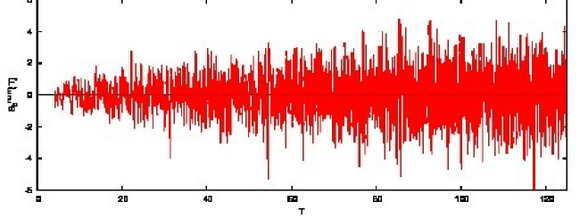
Figure 2. The fluctuations $S^{\text{num}}_{5}(T)$ for $\Gamma_{0}(5)^{+}$.

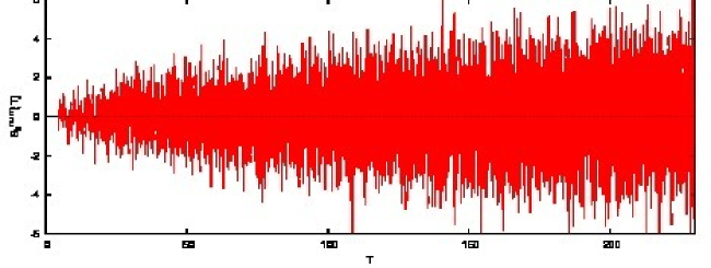
Figure 3. The fluctuations $S^{\text{num}}_{6}(T)$ for $\Gamma_{0}(6)^{+}$.

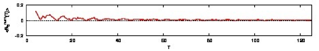
Figure 4. The mean $\langle S^{\text{num}}_{5}(T)\rangle$.

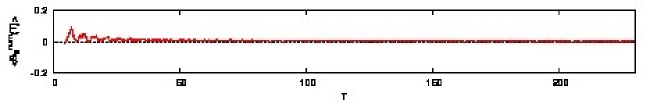
Figure 5. The mean $\langle S^{\text{num}}_{6}(T)\rangle$.

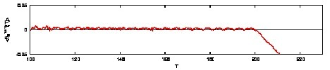
Figure 6. Mean $\langle S^{\text{num}}_{6}(T)\rangle$, with the eigenvalue $\lambda_{9367}=200.0359^{2}+1/4$ removed.

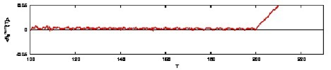
Figure 7. Mean $\langle S^{\text{num}}_{6}(T)\rangle$, with the fake “eigenvalue” $\lambda=200^{2}+1/4$ inserted.

Figures 2 and 3 show the fluctuations $S^{\text{num}}_{N}(T)$. In figures 4 and 5, the mean

$$\langle S^{\text{num}}_{N}(T)\rangle:=\frac{1}{T}\int\limits_{0}^{T}S^{\text{num}}_{N}(t)dt$$

tends to zero for large $T$ which indicates that all solutions have been found numerically.

If a solution would have been overlooked, the graph would deviate from zero quite significantly. A demonstration is given in figure 6, where we have intentionally removed the eigenvalue $\lambda_{9367}=200.0359^{2}+1/4$, whereas in figure 7, we have intentionally inserted a fake “eigenvalue” at $\lambda=200^{2}+1/4$.

If we would have an explicit and efficient upper bound on $\int\limits_{0}^{T}S_{N}(t)dt$, we could apply Turing’s method to prove, not just verify, that the numerically found lists of eigenvalues are consecutive. The proof would be to add a fake “eigenvalue” near the end of each list of eigenvalues and show that with this extra “eigenvalue” $\langle S^{\text{num}}_{N}(T)\rangle$ would exceed the upper bound, as explained in section 2.7, see also [33, 6, 8]. In our notation, what is needed is to explicitly evaluate the implied constant in the average of $S_{N}(T)$. The algorithm in [14] and [22] does, in fact provide such a bound, but the explicit value is somewhat large, hence impractical.

Remark 19.

For computing $S^{\text{num}}_{N}(T)$ we need to evaluate $\mathcal{M}_{N}(T)$ which includes the term $G_{N}(T)$. Actually, we do not know the exact value of $G_{N}(T)$. According to the bound (1), we can safely neglect $G_{N}(T)$ in the evaluation of $S^{\text{num}}_{N}(T)$ for $T$ large.

By Theorem 1, $\mathcal{M}_{N}(T)$ includes terms which depend on $\alpha_{N}(j,T)$ and on $\arctan(\cdot)$. For evaluating the average $\langle S^{\text{num}}_{N}(T)\rangle$, we need to integrate over these terms. The sum of the $\alpha_{N}(j,T)$ and the $\arctan(\cdot)$ dependent terms is periodic. We perform the integration by expanding the periodic contribution into a Fourier series, integrate the individual Fourier terms, and then sum up numerically.

4.2. Nearest neighbour spacing statistics

Concerning the statistical properties of the eigenvalues, we must emphasize that the conjectured properties depend on the choice of the surface $X$. Depending on whether the corresponding classical system of a point particle that moves freely on the surface is integrable or not, there are some generally accepted conjectures about the nearest neighbour spacing distributions of the eigenvalues in the limit $\lambda\to\infty$.

Whenever we examine the distribution of the eigenvalues we consider the values on the scale of the mean level spacings.

Conjecture 20 ([2]).

If the corresponding classical system is integrable, the eigenvalues behave like independent random variables and the distribution of the nearest neighbour spacings is in the limit $\lambda\to\infty$ close to a Poisson distribution, i.e. there is no level repulsion.

Conjecture 21 ([4]).

If the corresponding classical system is chaotic, the eigenvalues are distributed like the eigenvalues of hermitian random matrices. The corresponding ensembles depend only on the symmetries of the system:

• For chaotic systems without time-reversal invariance the distribution of the eigenvalues approaches in the limit $\lambda\to\infty$ the distribution of the Gaussian Unitary Ensemble (GUE) which is characterised by a quadratic level repulsion.

• For chaotic systems with time-reversal invariance and integer spin the distribution of the eigenvalues approaches in the limit $\lambda\to\infty$ the distribution of the Gaussian Orthogonal Ensemble (GOE) which is characterised by a linear level repulsion.

• For chaotic systems with time-reversal invariance and half-integer spin the distribution of the eigenvalues approaches in the limit $\lambda\to\infty$ the distribution of the Gaussian Symplectic Ensemble (GSE) which is characterised by a quartic level repulsion.

These conjectures are very well confirmed by numerical calculations, but several exceptions are known.

Exception 22.

The harmonic oscillator is classically integrable, but its spectrum is equidistant.

Exception 23.

The geodesic motion on surfaces with constant negative curvature provides a prime example for classical chaos. In some cases, however, the nearest neighbour distribution of the eigenvalues of the Laplacian on these surfaces appears to be Poissonian.

With our lists of consecutive eigenvalues, we can examine the nearest neighbour spacings. We unfold the spectrum

$$u_{n}=\mathcal{M}_{N}(r_{n})\ \text{ with }\ \lambda_{n}=r_{n}^{2}+1/4,$$

in order to obtain rescaled eigenvalues $u_{n}$ with a unit mean density. Then

$$s_{n}=u_{n+1}-u_{n}$$

defines the sequence of nearest neighbour level spacings which has a mean value of $1$ as $n\to\infty$. For the moonshine groups $\Gamma_{0}(5)^{+}$ and $\Gamma_{0}(6)^{+}$ we find that the spacing distributions come close to that of a Poisson random process,

$$P_{\text{Poisson}}(s)=e^{-s},$$

see figure 8, as opposed to that of a Gaussian orthogonal ensemble of random matrix theory,

$$P_{\text{GOE}}(s)\simeq\frac{\pi}{2}se^{-\frac{\pi}{2}s^{2}}.$$

The spacing distributions are in accordance with Conjecture 3.

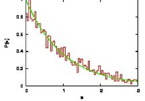
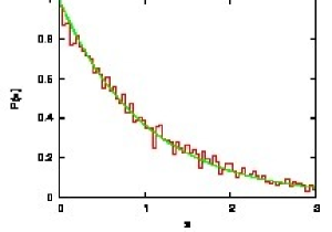
Figure 8. Nearest neighbour spacing distributions $P(s)$ for the moonshine groups $\Gamma_{0}(5)^{+}$ (left), and $\Gamma_{0}(6)^{+}$ (right), which come close the Poisson distribution $P_{\text{Poisson}}(s)=e^{-s}$.

One might wonder whether eigenvalue spacings are correlated. For this we investigated joint eigenvalue spacing distributions,

$$P(s,s^{\prime})dsds^{\prime}=P\big{(}(s_{n},s_{n+1})\in[s,s+ds)\times[s^{\prime},s^{\prime}+ds^{\prime})\big{)}.$$

For $\Gamma_{0}(5)^{+}$ and $\Gamma_{0}(6)^{+}$, we find that the joint eigenvalue spacing distributions factor into a product of Poisson distributions,

$$P(s,s^{\prime})=P_{\text{Poisson}}(s)P_{\text{Poisson}}(s^{\prime}),$$

see figures 9 and 10. Heuristically, the spacings between rescaled eigenvalues are uncorrelated which implies that the eigenvalues are uncorrelated as well.

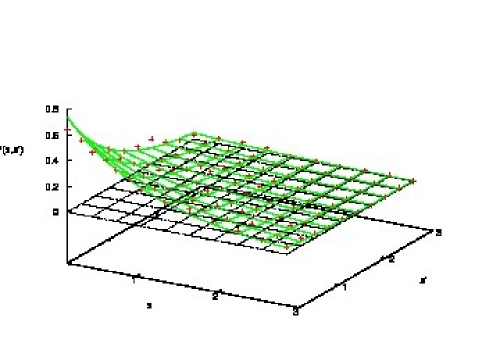
Figure 9. Joint nearest neighbour spacing distribution $P(s,s^{\prime})$ for $\Gamma_{0}(5)^{+}$ which comes close to a product of Poisson distributions $P_{\text{Poisson}}(s)P_{\text{Poisson}}(s^{\prime})$.

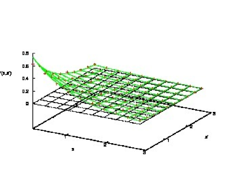
Figure 10. Joint nearest neighbour spacing distribution $P(s,s^{\prime})$ for $\Gamma_{0}(6)^{+}$ which comes close to the product of Poisson distributions $P_{\text{Poisson}}(s)P_{\text{Poisson}}(s^{\prime})$.

5. Concluding remarks

5.1. Topological equivalence versus Weyl’s law

The groups $\Gamma_{0}(5)^{+}$ and $\Gamma_{0}(6)^{+}$, which were the main focus of investigation in our paper, are topologically equivalent, have different Weyl’s law, yet the two sets of eigenvalues seem to have the same spacing distributions.

From the tables presented in [12], one can find other examples of such groups. In the case when the genus $g$ is zero, we have the following examples of topologically equivalent groups with different “classical” Weyl’s laws and “average” Weyl’s law.

1. For $N\in\{11,14,15\}$, the signature of the surface $\overline{\Gamma_{0}(N)^{+}}\backslash\mathbb{H}$ is $(0;2,2,2,2;1)$,

2. For $N\in\{17,22,30\}$, the signature of the surface $\overline{\Gamma_{0}(N)^{+}}\backslash\mathbb{H}$ is $(0;2,2,2,2,2;1)$,

3. For $N\in\{23,33,42\}$, the signature of the surface $\overline{\Gamma_{0}(N)^{+}}\backslash\mathbb{H}$ is $(0;2,2,2,2,2,2;1)$,

4. For $N\in\{29,38\}$, the signature of the surface $\overline{\Gamma_{0}(N)^{+}}\backslash\mathbb{H}$ is $(0;2,2,2,2,2,2,2;1)$,

5. For $N\in\{46,51,55,66,70\}$, the signature of the surface $\overline{\Gamma_{0}(N)^{+}}\backslash\mathbb{H}$ is $(0;2,2,2,2,2,2,2,2;1)$.

There are also examples of the groups with genus $g=1$, such as $N\in\{83,123,143,182,195\}$ each of which has signature $(1;2,2,2,2,2,2,2,2,2,2,2,2;1)$ and whose Weyl’s law asymptotics differ in the $T$ term.

This empirical investigation yields to an interesting question: For a given positive integer $k$, is it possible to find $k$ topologically equivalent surfaces arising from moonshine groups having different Weyl’s laws?

5.2. Weyl asymptotics versus nearest neighbour statistics

Generally speaking, discrete eigenvalues of the Laplacian, or, equivalently, positive imaginary parts of zeros of the corresponding Selberg zeta function on the critical line, are increasing sequences of numbers, and the associated Weyl’s law is an approximate counting function of such sequences. The results in section 4.2 are related to numerical computation of the nearest neighbour statistics of eigenvalues of Maass cusp forms on $\overline{\Gamma_{0}(N)^{+}}\backslash\mathbb{H}$, for $N=5$ and $N=6$. We have seen, empirically, that the nearest neighbour statistics for the eigenvalues of Maass cusp forms seem to be each equal even though the Weyl’s laws are different. One may argue that the reason for this is that the Weyl’s law differs in the $T$ term, while the first two lead terms are the same in the two cases we considered.

Therefore, a natural question which arises is to what extent does the nearest neighbour statistics of an increasing sequences of numbers depend on its average counting function. The answer to this question is presented in the following example.

Example 24.

Let $\{x_{n}\}_{n\in\mathbb{N}}$ be an increasing sequence of numbers having a mean density of $1$, by which we mean

$$\lim_{T\to\infty}\frac{1}{T}\#\{x_{n}\leq T\}=1.$$

Let $m(t)$ be an increasing function, defined for $t>0$, such that $m(0)\geq 1/2$. (In the Weyl’s law case, $m(t)=a_{0}t^{2}+a_{1}t\log t+a_{2}t+a_{3}+\ldots$, for some positive number $a_{0}$.) Let us define a sequence of numbers $\lambda_{n}$ by letting $\lambda_{n}:=m^{-1}(x_{n}-\frac{1}{2})$, where $m^{-1}$ denotes the inverse function of $m$. Let $\mathcal{N}(t)$ be the counting function

$$\mathcal{N}(t):=\#\{\lambda_{n}\leq t\},$$

and let the Weyl asymptotics $\mathcal{M}(t)$ be a smooth approximation to $\mathcal{N}(t)$ such that

$$\lim_{T\to\infty}\frac{1}{T}\int\limits_{0}^{T}(\mathcal{N}(t)-\mathcal{M}(t))dt=0.$$

The unfolded spectrum $\{u_{n}\}$ is defined by $u_{n}:=m(\lambda_{n})$. Trivially, $u_{n}=m(\lambda_{n})=m(m^{-1}(x_{n}-\frac{1}{2}))=x_{n}-\frac{1}{2}$, for all $n\in\mathbb{N}$ hence $u_{n+1}-u_{n}=x_{n+1}-x_{n}$, so the nearest neighbour statistics of the unfolded spectrum $\{u_{n}\}$ equals the nearest neighbour statistics of the initial sequence $\{x_{n}\}$.

We are free to distribute the sequence of increasing numbers $\{x_{n}\}$ such that the nearest neighbour statistics of $\{x_{n}\}$ coincides with our favorite distribution of non-negative numbers. We are also free to choose the smooth increasing function $m(t)$, and hence the Weyl asymptotics arbitrarily. Since $\{x_{n}\}$ and $m(t)$ can be chosen independently of each other, we conclude that the nearest neighbour statistics of the unfolded spectrum $\{u_{n}\}$ is completely independent of the Weyl asymptotics.

Therefore, all the analytic results on the Weyl asymptotics are completely independent of the numerical results on the nearest neighbour statistics. Neither carries any information of the other, regardless of how many expansion terms we include in the Weyl asymptotics. Analytics and numerics complement each other.

References

• [1] A. O. L. Atkin and J. Lehner, Hecke operators on $\Gamma_{0}(m)$, Math. Ann. 185 (1970), 134–160.
• [2] M. V. Berry and M. Tabor, Closed orbits and the regular bound spectrum, Proc. R. Soc. London A 349 (1976), 101–123.
• [3] E. B. Bogomolny, B. Georgeot, M.-J. Giannoni, and C. Schmit, Chaotic billiards generated by arithmetic groups, Phys. Rev. Lett. 69 (1992), 1477–1480.
• [4] O. Bohigas, M.-J. Giannoni, and C. Schmit, Spectral fluctuations, random matrix theories and chaotic motion. Stochastic processes in classical and quantum systems, Lecture Notes in Phys. 262 (1986), 118–138.
• [5] J. Bolte, G. Steil, and F. Steiner, Arithmetical chaos and violation of universality in energy level statistics, Phys. Rev. Lett. 69 (1992), 2188–2191.
• [6] A. R. Booker, Turing and the Riemann hypothesis, AMS Notices 53 (2006), 1208–1211.
• [7] A. R. Booker and A. Strömbergsson, Numerical computations with the trace formula and the Selberg eigenvalue conjecture, J. Reine Angew. Math. 607 (2007), 113–161.
• [8] A. R. Booker and A. Strömbergsson, Theoretical and practical aspects of Maass form computations, in preparation.
• [9] A. R. Booker, A. Strömbergsson and A. Venkatesh, Effective computation of Maass cusp forms, IMRN, 2006 (2006); Article ID 71281, 34 pp.
• [10] J. Conway, J. McKay, A. Sebbar, On the discrete groups of Moonshine, Proc. Amer. Math. Soc. 132 (2004), 2233–2240.
• [11] C. J. Cummins and T. Gannon, Modular equations and the genus zero property of moonshine functions, Invent. Math. 129 (1997), 413–443.
• [12] C. J. Cummins, Congruence subgroups of groups commensurable with $\operatorname{PSL}(2,\mathbb{Z})$ of genus 00 and $1$, Exper. Math. 13 (2004), 361–382.
• [13] C. J. Cummins, Fundamental domains for genus-zero and genus-one congruence subgroups, LMS J. Comput. Math. 13 (2010), 222–245.
• [14] J. Friedman, J. Jorgenson, and J. Kramer An effective bound for the Huber constant for cofinite Fuchsian groups, Math. Comp. 80 (2011), 1163–1196.
• [15] T. Gannon, Moonshine Beyond the Monster. The Bridge Connecting Algebra, Modular Forms and Physics, Cambridge Monographs on Mathematical Physics, Cambridge University Press, Cambridge, 2006.
• [16] I. S. Gradshteyn and I. M. Ryzhik, Table of Integrals, Series and Products, Elsevier Academic Press, Amsterdam, 2007.
• [17] D. A. Hejhal, The Selberg Trace Formula for $\operatorname{PSL}(2,\mathbb{R})$, Volume 2. Lecture Notes in Math. 1001, Springer-Verlag, New York, 1983.
• [18] D. A. Hejhal, On eigenfunctions of the Laplacian for Hecke triangle groups. In D. A. Hejhal, J. Friedman, M. C. Gutzwiller, and A. M. Odlyzko, Emerging Applications of Number Theory, IMA Series No. 109, Springer-Verlag, New York, 1999, pp. 291–315.
• [19] H. Helling, Bestimmung der Kommensurabilitätsklasse der Hilbertschen Modulgruppe, Math. Z. 92 (1966), 269–280.
• [20] M. N. Huxley, Scattering matrices for congruence subgroups, In R. A. Rankin, Modular forms. Ellis Horwood, Chichester, 1984, pp. 141–156.
• [21] H. Iwaniec, Spectral Methods of Automorphic Forms, Graduate Studies in Mathematics 53, AMS, Providence 2002.
• [22] J. Jorgenson and J. Kramer, On the error term of the prime geodesic theorem, Forum Math. 14 (2002), 901–913.
• [23] J. Jorgenson and L. Smajlović, On the distribution of zeros of the derivative of the Selberg’s zeta function associated to finite volume Riemann surfaces, preprint (2012).
• [24] H. Maaß, Über eine neue Art von nichtanalytischen automorphen Funktionen und die Bestimmung Dirichletscher Reihen durch Funktionalgleichungen, Math. Ann. 121 (1949), 141–183.
• [25] R. S. Phillips and P. Sarnak, On cusp forms for co-finite subgroups of $\operatorname{PSL}(2,R)$, Invent. Math. 80 (1985), 339–364.
• [26] P. Sarnak, Spectra of hyperbolic surfaces, Bull. Amer. Math. Soc. 40 (2003), 441–478.
• [27] G. Shimura, Introduction to the Arithmetic Theory of Automorphic Forms, Publications of the Mathematical Society of Japan, Princeton University Press, Princeton, 1971.
• [28] F. Strömberg, Maass waveforms on $(\Gamma_{0}(N),\chi)$ (computational aspects). In J. Bolte and F. Steiner, Hyperbolic Geometry and Applications in Quantum Chaos and Cosmology, LMS Lecture Note Series 397, Cambridge University Press, Cambridge, 2011, pp. 187–228.
• [29] A. Strömbergsson, A pullback algorithm for general (cofinite) Fuchsian groups, (2000), http://www2.math.uu.se/~astrombe/papers/pullback.ps.
• [30] H. Then, Maass cusp forms for large eigenvalues, Math. Comp. 74 (2005), 363–381.
• [31] H. Then, Computing large sets of consecutive Maass forms, in preparation.
• [32] E. C. Titchmarsh, The Theory of the Riemann Zeta-Function, 2nd ed., revised by D. R. Heath-Brown, Oxford University Press, New York, 1986.
• [33] A. M. Turing, Some calculations of the Riemann zeta-function, Proc. London Math. Soc. 3 (1953), 99–117.