Abstract

A status report on the topic nucleon Compton scattering and polarizabilities is presented with emphasis on the scalar $t$-channel as entering into dispersion theory. Precise values for the polarizabilities are obtained leading to $\alpha_{p}=12.0\pm 0.6$ ($12.0$), $\beta_{p}=1.9\mp 0.6$ ($1.9$), $\alpha_{n}=12.5\pm 1.7$ ($13.4$), $\beta_{n}=2.7\mp 1.8$ ($1.8$) in units of $10^{-4}$ fm³ and $\gamma^{(p)}_{\pi}=-36.4\pm 1.5$ ($-36.6$), $\gamma^{(n)}_{\pi}=58.6\pm 4.0$ ($58.3$), ($\gamma^{(p)}_{0}=-0.58\pm 0.20$), ($\gamma^{(n)}_{0}=+0.38\pm 0.22$) in units of $10^{-4}$ fm⁴, for the proton $(p)$ and neutron $(n)$, respectively. The data given with an error are $recommended$ experimental values with updates compared to [1] where necessary, the data in parentheses are predicted values. These predicted values are not contained in [1], but are the result of a newly developed analysis which is the main topic of the present paper. The most important recent discovery is that the largest part of the electric polarizability and the total diamagnetic polarizability of the nucleon are properties of the $\sigma$ meson as part of the constituent-quark structure, as expected from the mechanism of chiral symmetry breaking. This view is supported by an experiment on Compton scattering by the proton carried out in the second resonance region, where a large contribution from the $\sigma$ meson enters into the scattering amplitudes. This experiment led to a determination of the mass of the $\sigma$ meson of $m_{\sigma}=600\pm 70$ MeV. From the experimental $\alpha_{p}$ and predicted differences $(\alpha_{n}-\alpha_{p})$ neutron polarizabilities in the range $\alpha_{n}=12.0-13.4$ are predicted, where the uncertainties are related to the $f_{0}(980)$ and $a_{0}(980)$ scalar mesons.

1 Introduction

The idea to apply the coherent elastic scattering of photons (Compton scattering ) to an investigation of the internal structure of the nucleon dates back to the early 1950s. At that time the structure of the nucleon was mainly discussed in terms of a bare nucleon surrounded by a “pion cloud”. In the framework of this simple model the polarization of the pion cloud leads to an absorption of the incoming photon and the emision of the outgoing photon and thus to a Compton scattering process. Estimates carried out by Sachs and Foldy in 1950 showed that the pion-cloud polarization should lead to a small modification of the Thomson scattering cross section [2]. Later on in 1957 the proposal was made by Aleksandrov [3] to measure cross sections for the scattering of slow neutrons in the Coulomb field of heavy nuclei. In this case it was predicted that the pion-cloud polarization leads to a small modification of Schwinger’s scattering cross section which takes into account the effects of the anomalous magnetic moment of the neutron. For the proton the scattering in a Coulomb field is no option because of the electric charge of the proton.

The first experiment on Compton scattering by the proton to measure the polarizability was carried out in 1958. The final experiment of high precision was performed at MAMI (Mainz) by Olmos de León et al in 2001 [4]. An extensive description of these experiments and their analyses may be found in [1, 5, 6, 7] The weighted averages of these results are given in Table 1 of the present work.

First experiments on electromagnetic scattering of slow neutrons have been carried out from 1986 to 1988. The results of these experiments are listed in Table 2 of [1]. These first experiments remained of rather limited precision. Great progress has been made in an experiment carried out by Schmiedmayer et al. in 1991 [8]. The result obtained in [8] is discussd in subsection 2.6 of the present paper.

As a second option to measure the electromagnetic polarizabilities of the neutron quasifree Compton scattering by a neutron bound in a deuteron has been proposed by Levchuk et al. [9]. In this case only the internal structure of the neutron is excited whereas the proton merely serves as a spectator. The first high-precision experiment of this kind has been carried out by Kossert et al. in 2002 [10], leading to a result which is discussed in subsection 2.6 of the present paper together with the result of electromagnetic scattering of neutrons [8].

In principle also the cohenrent elastic Compton scattering by the deuteron may be exploited. In this case the sum of the proton and neutron polarizabilities is measured which may be used to arrive at the polarizability of the neutron by subtracting the proton polarizability. A first experiment of this kind has ben carried out by Lundin et al. [11] and it has been proposed to repeat the experiment in order to arrive at a higher precision [12]

1.1 Theoretical approaches to the polarizabilities of the nucleon

A number of theoretical papers concerned with the polarizabilities of the nucleon based on nucleon models have been published in the 1980s. These investigations include the MIT bag model, the nonrelativistic quark model, the chiral quark model, the chiral soliton model and the Skyrme model. The investigations based nucleon models ceased with the advent of effective field theories at the beginning of the 1990s. These latter theories attracted many researchers and still are a subject of active investigations. Some information on the early activities may be found in [13, 7, 1]. For the status of the present activities we wish to cite the recent article “Using effective field theory to analysis low-energy Compton scattering data from protons and light nuclei” [14] and “Signatures of chiral dynamics in low-energy Compton scattering off the nucleon” [15]. In the analyses described in [14] the polarizabilities are treated as free parameters. The results obtained may be compared with the present recommended values. In [15] a projection formalism is presented which allows to define dynamical polarizabilities of the nucleon from a multipole expansion of the nucleon Compton amplitudes. These dynamical polarizabilities may be compared with the corresponding quantities presented in section 6 of the present work. Since these investigations [14, 15] have been published recently, the papers cited therein should give a complete overview.

1.2 Outline of the present article

The purpose of the present article is to give a concise status report on the research topic of nucleon Compton scattering and polarizabilities, by describing the results achieved on the basis of dispersion theory since the latest review article published in 2005 [1], partly based on published and partly on recent unpublished investigations. The published results are distributed over a larger number of papers [16, 17, 18, 19, 20, 21, 22, 23]. This makes it difficult for the reader to get insight into the present status of development and makes a status report on the results highly advisable.

The present status report includes a complete precise prediction of the polarizabilities and their interpretation in terms of degrees of freedom of the nucleon. The progress made for the prediction of the nucleon structure ($s$-channel) part has been made possible by high-precision analyses [24] of photomeson data and their conversion into partial photoabsorption cross sections for all resonant and nonresonant photoexcitation processes of the nucleon [20, 22]. These high-precision analyses contain the most precise information on the electromagnetic structure of the nucleon available at present. Using dispersion relations these partial photoabsorption cross sections can be transferred into polarizabilities. As a consequence we have a method to precisely predict the polarizabilities of the nucleon on the basis of meson photoproduction data which includes all processes which are considered as the degrees of freedom of the nucleon. However, when carrying out these predictions of electromagnetic polarizabilities one is led to a severe problem. The electric polarizability $\alpha$ predicted in this way amounts to only about 40% of the experimental value and the magnetic polarizability $\beta$ overshoots the experimental value by about a factor of 5. Apparently there is a missing piece in the electric polarizability and a strong diamagnetic component which compensates the predicted paramagnetic polarizability.

Predictions based on models of the nucleon are in general not sensitive to details of the problems outlined above. On the other hand, already in 1974 T.E.O. Ericson and coworkers (BEFT) [25, 26] carried out calculations on the basis of dispersion relations which led to the discovery of the missing piece in the electric polarizability and to the missing diamagnetic polarizability. These authors found a way of solving this severe problem by tracing it back to the scalar $t$-channel contribution introduced by Hearn and Leader in 1962 [27, 28]. Quantitatively, the results obtained in [25, 26] remained of rather limited precision. Therefore, in the following years further calculations were carried out by a number of researchers with more or less success as far as the numerical results are concerned. The main problem persisting up to the present was to get data of sufficient precision for the scalar two-photon excitation process leading to a pion pair in the final state. This line of development is described in detail in the previous review [1].

In [1] a step further is made by asking the question how this scalar $t$-channel can be understood in terms of degrees of freedom of the nucleon, a question which had never been asked before. Since the structure of the nucleon as observed in photomeson experiments is exhausted by the $s$-channel it was considered as likely that the $t$-channel is related to the mesonic structure of the constituent quarks. This idea was worked out in a series of investigations [16, 17, 18, 19, 20, 21, 22, 23] and proved to be extremely successful after it had been noted that the quark-level linear $\sigma$ model (QLL$\sigma$M) as developed by Delbourgo, Scadron and coworkers [29, 30, 31] leads to a quantitative agreement with the experimental data. In this way the missing part of the electric polarizability and the diamagnetic polarizability were traced back to the $\sigma$ meson as part of the constituent-quark structure. From the point of view of chiral symmetry breaking this does not come as a surprise. Chiral symmetry breaking explains the mass of the constituent quark in terms of the exchange of the $\sigma$ meson with $q\bar{q}$ loops of the QCD vacuum. This necessarily leads to a $\sigma$ meson as part of the constituent-quark structure.

The nucleon model introduced above containing a $\sigma$ meson as part of the constituent-quark structure is strongly supported by a Compton scattering experiment on the proton carried out at MAMI (Mainz) in the 1990s and published in 2001 [32, 33]. In this experiment it has been shown that the scalar $t$-channel makes a strong contribution to the Compton scattering amplitude in the second resonance region of the nucleon at large scattering angles. This contribution is successfully represented in terms of a $t$-channel pole located at $m^{2}_{\sigma}$ as introduced by L‘vov et al. in 1997 [34] where $m_{\sigma}$ is the “bare” mass of the $\sigma$ meson, determined in this experiment to be $m_{\sigma}=600\pm 70$ MeV. The error given here corresponds to the uncertainty of the CGLN amplitude representing the $P_{33}(1232)$ resonance. Details are given in section 6. In spite of this great success the physical interpretation of the experiment remained uncertain because the $\sigma$ meson was not a generally accepted particle at that time. This led to a delay in the final interpretation of the experiment, because additional detailed theoretical investigations were required in oder to remove the remaining uncertainties. The breakthrough came in 2006 [16] when it was shown that it is possible to quantitatively predict the scalar $t$-channel part of the electromagnetic polarizabilities in terms of the QLL$\sigma$M and thus proving that the $t$-channel part of the Compton-scattering amplitude is a property of the structure of the constituent quarks. This result was further worked out in a series of additional investigation [17, 18, 19, 20, 21, 22].

In the course of these further investigations it was realized that the $\sigma$ meson provides by far the largest part of the scalar $t$-channel contribution. But there are also smaller contributions from the $f_{0}(980)$ and $a_{0}(980)$ scalar mesons. These mesons together with the $\sigma$ meson are members of the scalar nonet $\sigma(600)$, $\kappa(800)$, $f_{0}(980)$ $a_{0}(980)$. This observation led to the attempt to extend the QLL$\sigma$M of [29, 30, 31] to SU(3). The investigation carried out in [23] showed that the members of the scalar nonet have the same mass in the chiral limit (cl) amounting to $m^{\rm cl}_{\sigma}=652$ MeV. This degeneracy is removed via explicit symmetry breaking by taking into account the effects of the finite current-quark masses, applying the rules of spontaneous and dynamical symmetry breaking.

The present review is organized as follows. In section 2 we present an updated list of recommended experimental values for the polarizabilities. New arguments are given in favor of the value $\alpha_{n}=(12.5\pm 1.7)\times 10^{-4}$fm³ of the neutron electric polarizability. A slight modification of the recommended value of $\gamma^{(p)}_{\pi}$ is found. In section 3 we derive a complete list of predicted contributions to the $s$-channel polarizabilities. In section 4 we describe the properties of the invariant amplitudes and their relation to the polarizabilities. Section 5 is concerned with the $t$-channel polarizabilities. Since the methods and results for the $t$-channel are widely unknown we provide an extended description of the $t$-channel aimed to arrive at high clarity. In section 6 we describe Compton scattering in a large angular range and at energies up to 1 GeV, with emphasis on interference effects between nucleon structure ($s$-channel) and constituent-quark structure ($t$-channel) contributions.

2 Definition of polarizabilities and compilation of experimental results

In the following we will outline the basic relations used in our studies of nucleon Compton scattering and polarizabilities beginning with a classic approach to the polarizabilities. We will see that in addition to the electromagnetic polarizabilities $\alpha$ and $\beta$ spin-polarizabilities $\gamma_{0}$ and $\gamma_{\pi}$ for Compton scattering in the forward and backward directions are required. The experiments and the experimental results have been described in previous works [5, 1]. This makes it sufficient for the present review to only summarize the experimental results

2.1 Polarizabilities and electromagnetic fields

A nucleon in an electric field ${\bf E}$ and magnetic field ${\bf H}$ obtains an induced electric dipole moment ${\bf d}$ and magnetic dipole moment ${\bf m}$ given by

$${\bf d}=4\pi\,\alpha\,{\bf E},$$ (1)

$${\bf m}=4\pi\,\beta\,{\bf H},$$ (2)

in a unit system where the electric charge $e$ is given by $e^{2}/4\pi=\alpha_{em}=1/137.04$. Eqs. (1) and (2) may be understood as the response of the nucleon to the fields provided by a real or virtual photon and it is evident that we need a second photon to measure the polarizabilities. This may be expressed through the relation

$$H^{(2)}=-\frac{1}{2}\,4\pi\,\alpha\,{\bf E}^{2}-\frac{1}{2}\,4\pi\,\beta\,{\bf H}^{2}$$ (3)

where $H^{(2)}$ is the energy change in the electromagnetic field due to the presence of the nucleon in the field.

2.2 Forward and backward Compton scattering

Compton scattering contains the most effective method to provide two photons interacting simultaneously with the nucleon. Therefore, Compton scattering is the method of first choice for the measurement of polarizabilities. The second method is the electromagnetic scattering of slow neutrons in the electric field of a heavy nucleus.

The differential cross section for Compton scattering

$$\gamma N\to\gamma^{\prime}N^{\prime}$$ (4)

may be written in the form [35]

$$\frac{d\sigma}{d\Omega}=\Phi^{2}|T_{fi}|^{2}$$ (5)

with $\Phi=\frac{1}{8\pi M}\frac{\omega^{\prime}}{\omega}$ in the lab frame ($\omega$, $\omega^{\prime}$ = lab energies of the incoming and outgoing photon) and $\Phi=\frac{1}{8\pi\sqrt{s}}$ in the cm frame ($\sqrt{s}$ = total energy). For the following discussion it is convenient to use the lab frame and to consider special cases for the amplitude $T_{fi}$. These special cases are the extreme forward ($\theta=0$) and extreme backward ($\theta=\pi$) direction where the amplitudes for Compton scattering may be written in the form [35]

$$\frac{1}{8\pi m}[T_{fi}]_{\theta=0}=f_{0}(\omega){\mbox{\boldmath$\epsilon$}}^{\prime}{}^{*}\cdot{\mbox{\boldmath$\epsilon$}}+g_{0}(\omega)\,\mbox{i}\,{\mbox{\boldmath$\sigma$}}\cdot({\mbox{\boldmath$\epsilon$}}^{\prime}{}^{*}\times{\mbox{\boldmath$\epsilon$}}),$$ (6)

$$\frac{1}{8\pi m}[T_{fi}]_{\theta=\pi}=f_{\pi}(\omega){\mbox{\boldmath$\epsilon$}}^{\prime}{}^{*}\cdot{\mbox{\boldmath$\epsilon$}}+g_{\pi}(\omega)\,\mbox{i}\,{\mbox{\boldmath$\sigma$}}\cdot({{\mbox{\boldmath$\epsilon$}}}^{\prime}{}^{*}\times{{\mbox{\boldmath$\epsilon$}}}),$$ (7)

with $m$ being the nucleon mass, $\epsilon$ the polarization of the photon and $\sigma$ the spin vector.

The process described in (6) is the transmission of linearly polarized photons through a medium as provided by a nucleon with spin vector $\sigma$ parallel or antiparallel to the direction of the incident photon with rotation of the direction of linear polarization. The amplitudes $f_{0}$ and $g_{0}$ correspond to the polarization components of the outgoing photon parallel and perpendicular to the direction of linear polarization of the incoming photon. The interpretation of (7) is the same as that of (6) except for the fact that the photon is reflected. In case of forward scattering (6) the origin of the rotation of the direction of linear polarization may be related partly to the alignment of the internal magnetic dipole moments of the nucleon and partly to the dynamics of the pion cloud. In case of backward scattering (7) a large portion of the relevant phenomenon is of a completely different origin. This is the $t$-channel contribution which will be studied in detail in the following. It is important to realize that in contrast to frequent belief there is no flip of any spin in the two cases of Compton scattering. The factor $\sigma$ in the second terms of the two equations may be interpreted as a spin dependence of scattering in the sense that the direction of rotation of the electric vector changes sign (from $e.g.$ clock-wise to anti clock-wise) when the spin of the target nucleon is reversed.

The two scattering processes may also be related to the two states of circular polarization, i.e. helicity amplitudes for forward and backward Compton scattering. If the photon and nucleon spins are parallel (photon helicity $\lambda_{\gamma}=+1$, nucleon helicity $\lambda_{N}=-\frac{1}{2}$, and net helicity in the photon direction $\lambda=\lambda_{\gamma}-\lambda_{N}=\frac{3}{2}$) then the amplitude is

$$f^{3/2}_{0}(\omega)=f_{0}(\omega)-g_{0}(\omega),$$ (8)

while for the spins being anti-parallel (photon helicity $\lambda_{\gamma}=+1$, nucleon helicity $\lambda_{N}=+\frac{1}{2}$, and net helicity along the photon direction $\lambda=\lambda_{\gamma}-\lambda_{N}=+\frac{1}{2}$) the amplitude is

$$f^{1/2}_{0}(\omega)=f_{0}(\omega)+g_{0}(\omega).$$ (9)

The amplitudes $f^{3/2}_{0}$ and $f^{1/2}_{0}$ are related by the optical theorem to the total cross sections $\sigma_{3/2}$ and $\sigma_{1/2}$ for the reaction

$$\gamma+N\to N^{*}\to N+{\rm mesons}+\mbox{radiative decay of N${}^{*}$}$$ (10)

when the photon spin is parallel or anti-parallel to the nucleon spin:

$${\rm Im}f^{3/2}_{0}(\omega)=\frac{\omega}{4\pi}\sigma_{3/2}(\omega),$$ (11)

$${\rm Im}f^{1/2}_{0}(\omega)=\frac{\omega}{4\pi}\sigma_{1/2}(\omega).$$ (12)

Therefore,

$${\rm Im}\,f_{0}(\omega)=\frac{\omega}{4\pi}\,\frac{\sigma_{1/2}(\omega)+\sigma_{3/2}(\omega)}{2}=\frac{\omega}{4\pi}\sigma_{\rm tot}(\omega),$$ (13)

$${\rm Im}\,g_{0}(\omega)=\,\frac{\omega}{4\pi}\frac{\sigma_{1/2}(\omega)-\sigma_{3/2}(\omega)}{2}=\frac{\omega}{8\pi}\,\Delta\sigma(\omega),$$ (14)

where $\sigma_{\rm tot}(\omega)=(\sigma_{1/2}+\sigma_{3/2})/2$ is the spin averaged total cross section and $\Delta\sigma=\sigma_{1/2}-\sigma_{3/2}$. For the backward direction we obtain

$${\rm Im}f_{\pi}(\omega) = \frac{\omega}{4\pi}\left[\sigma(\omega,\Delta P={\rm yes})-\sigma(\omega,\Delta P={\rm no})\right],$$ (15)

$${\rm Im}g_{\pi}(\omega) = \frac{\omega}{8\pi}\left[\Delta\sigma(\omega,\Delta P={\rm yes})-\Delta\sigma(\omega,\Delta P={\rm no})\right],$$ (16)

$$\equiv \frac{\omega}{8\pi}\{[\sigma_{1/2}(\omega,\Delta P={\rm yes})-\sigma_{1/2}(\omega,\Delta P={\rm no})],$$

$$\,\,\,\,\,\,-[\sigma_{3/2}(\omega,\Delta P={\rm yes})-\sigma_{3/2}(\omega,\Delta P={\rm no})],\}$$

$$\equiv \frac{\omega}{8\pi}\sum_{n}P_{n}[\sigma^{n}_{3/2}(\omega)-\sigma^{n}_{1/2}(\omega)]$$

with $P_{n}=+1$ for $\Delta P=$ no (no parity change) and $P_{n}=-1$ for $\Delta P=$ yes (with parity change). Details of the derivation may be found in [1].

2.3 Definition of polarizabilities

Following Babusci et al. [35] the equations (6) and (7) can be used to define the electromagnetic polarizabilities and spin-polarizabilities as the lowest-order coefficients in an $\omega$-dependent development of the nucleon-structure dependent parts of the scattering amplitudes:

$$f_{0}(\omega) = -({e^{2}}/{4\pi m})Z^{2}+{\omega}^{2}({\alpha}+{\beta})+{\cal O}({\omega}^{4}),$$ (17)

$$g_{0}(\omega) = \omega\left[-({e^{2}}/{8\pi m^{2}})\,{\kappa}^{2}+{\omega}^{2}{\gamma_{0}}+{\cal O}({\omega}^{4})\right],$$ (18)

$$f_{\pi}(\omega) = \left(1+({\omega^{\prime}\omega}/{m^{2}})\right)^{1/2}[-({e^{2}}/{4\pi m})Z^{2}+\omega\omega^{\prime}({\alpha}-{\beta})+{\cal O}({\omega}^{2}{{\omega}^{\prime}}^{2})],$$ (19)

$$g_{\pi}(\omega) = \sqrt{\omega\omega^{\prime}}[({e^{2}}/{8\pi m^{2}})({\kappa}^{2}+4Z{\kappa}+2Z^{2})+\omega\omega^{\prime}{{\gamma_{\pi}}}+{\cal O}({\omega}^{2}{{\omega}^{\prime}}^{2})],$$ (20)

where $Ze$ is the electric charge ($e^{2}/4\pi=1/137.04$), $\kappa$ the anomalous magnetic moment of the nucleon and $\omega^{\prime}=\omega/(1+\frac{2\omega}{m})$.

In the relations for $f_{0}(\omega)$ and $f_{\pi}(\omega)$ the first nucleon structure dependent coefficients are the photon-helicity non-flip $(\alpha+\beta)$ and photon-helicity flip $(\alpha-\beta)$ linear combinations of the electromagnetic polarizabilities $\alpha$ and $\beta$. In the relations for $g_{0}(\omega)$ and $g_{\pi}(\omega)$ the corresponding coefficients are the spin polarizabilities $\gamma_{0}$ and $\gamma_{\pi}$, respectively.

2.4 Interpretation of Compton scattering in terms of electric and magnetic fields

Polarizabilities may be measured by simultaneous interaction of two photons with the nucleon. In case of static fields this may be written in the form given by Eq. (3). The first part on the r.h.s. of Eq. (3) is realized in experiments where slow neutrons are scattered in the electric field of a heavy nucleus, leading to a measurement of the electric polarizability as described by Eq. (40). The scattering of slow neutrons in the electrostatic field of a heavy nucleus corresponds to the encircled upper part of panel (1) in Figure 1, showing two parallel electric vectors. Only this case is accessible with longitudinal photons at low particle velocities. Compton scattering in the forward and backward directions leads to more general combinations of electric and magnetic fields. This is depicted in the four panels of Figure 1.

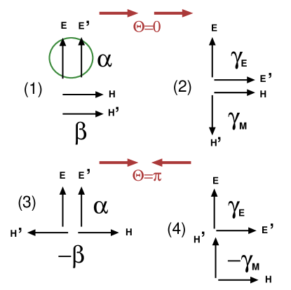
Figure 1: Compton scattering viewed as simultaneous interaction of two electric field vectors ${\bf E,E^{\prime}}$ and magnetic field vectors ${\bf H,H^{\prime}}$ for four different cases. (1) Helicity independent forward Compton scattering as given by the amplitude $f_{0}(\omega)$. (2) Helicity dependent forward Compton scattering as given by the amplitude $g_{0}(\omega)$. (3) Helicity independent backward Compton scattering as given by the amplitude $f_{\pi}(\omega)$. (4) Helicity dependent backward Compton scattering as given by the amplitude $g_{\pi}(\omega)$. Longitudinal photons can only provide two electric vectors with parallel planes of linear polarization as shown in the encircled upper part of panel (1). In panels (2) and (4) the direction of rotation leading from ${\bf E}$ to ${\bf E^{\prime}}$ depends on the helicity difference $|\lambda_{p}-\lambda_{\gamma}|$.

Panel (1) corresponds to the amplitude $f_{0}(\omega)$, panel (2) to the amplitude $g_{0}(\omega)$, panel (3) to the amplitude $f_{\pi}(\omega)$ and panel (4) to the amplitude $g_{\pi}(\omega)$. Panel (1) contains two parallel electric vectors and two parallel magnetic vectors. Through these the electric polarizability $\alpha$ and the magnetic polarizability $\beta$ can be measured. In panel (3) corresponding to backward scattering the direction of the magnetic vector is reversed so that instead of $+\beta$ the quantity $-\beta$ is measured. The nucleon has a spin and because of this the two electric and magnetic vectors have the option of being perpendicular to each other. This leads to the definition of the spin polarizability $\gamma$ which comes in different versions $\gamma_{E}$ and $\gamma_{M}$, respectively. The different directions of the magnetic field in the forward and backward direction leads to definitions of polarizabilities for the four cases

$$(1)\quad(\alpha+\beta)\hskip 42.67912pt\text{(forward polarizability)},$$ (21)

$$(2)\quad\gamma_{0}=\gamma_{E}+\gamma_{M}\hskip 14.22636pt\text{(forward spin-polarizability)},$$ (22)

$$(3)\quad(\alpha-\beta)\hskip 42.67912pt\text{(backward polarizability)},$$ (23)

$$(4)\quad\gamma_{\pi}=(\gamma_{E}-\gamma_{M})\hskip 5.69054pt\text{(backward spin-polarizability)}.$$ (24)

In former descriptions of Compton scattering and polarizabilities occasionally “Compton polarizabilities” $\overline{\alpha}$ and $\overline{\beta}$ have been introduced in order to distinguish them from the “static” polarizabilities $\alpha$ and $\beta$. The advantage of Figure 1 is that firm arguments are presented that a distinction of this kind is quite unnecessary.

2.5 Sum rules and $s$-channel polarizabilities

At this point it is useful to give expressions for sum rules which will be used later for the prediction of the polarizabilities. The following dispersion integrals have been derived:

$$\alpha+\beta=\frac{1}{2\pi^{2}}\int^{\infty}_{\omega_{0}}\frac{\sigma_{tot}(\omega)}{\omega^{2}}d\omega,$$ (25)

$$\gamma_{0}=-\frac{1}{4\pi^{2}}\int^{\infty}_{\omega_{0}}\frac{\sigma_{3/2}-\sigma_{1/2}}{\omega^{3}}d\omega,$$ (26)

$$(\alpha-\beta)^{s}=\frac{1}{2\pi^{2}}\int^{\infty}_{\omega_{0}}\sqrt{1+\frac{2\omega}{m}}[\sigma(\omega,\Delta P={\rm yes})-\sigma(\omega,\Delta P={\rm no})]\frac{d\omega}{\omega^{2}},$$ (27)

$$\gamma^{s}_{\pi}=\frac{1}{4\pi^{2}}\int^{\infty}_{\omega_{0}}\sqrt{1+\frac{2\omega}{m}}\left(1+\frac{\omega}{m}\right)\sum_{n}P_{n}[\sigma^{n}_{3/2}(\omega)-\sigma^{n}_{1/2}(\omega)]\frac{d\omega}{\omega^{3}}$$ (28)

where $P_{n}=+1$ for $\Delta P=$ no (no parity change) and $P_{n}=-1$ for $\Delta P=$ yes (with parity change). The sum rule for $(\alpha+\beta)$ is the Baldin-Lapidus (BL) sum rule [36], the sum rule for $\gamma_{0}$ a subtracted version of the Gerasimov-Drell-Hearn (GDH) sum rule [37], the sum rule for $(\alpha-\beta)^{s}$ the $s$-channel part of the Bernabeu et al. (BEFT) sum rule [25, 26] and the sum rule for $\gamma^{s}$ the $s$-channel part of the L’vov-Nathan (LN) sum rule [38]. The two latter sum rules have to be supplemented by $t$-channel pole terms as shown in the following.

The appropriate tool for the prediction of the polarizabilities $\alpha$ and $\beta$ is to simultaneously apply the forward-angle sum rule for $(\alpha+\beta)$ and the backward-angle sum rule for $(\alpha-\beta)$. This leads to the following relations [17, 20] :

$$\alpha=\alpha^{s}+\alpha^{t},$$ (29)

$$\alpha^{s}=\frac{1}{2\pi^{2}}\int^{\infty}_{\omega_{0}}\left[A(\omega)\sigma(\omega,E1,M2,\cdots)+B(\omega)\sigma(\omega,M1,E2,\cdots)\right]\frac{d\omega}{\omega^{2}},$$ (30)

$$\alpha^{t}=\frac{1}{2}(\alpha-\beta)^{t}$$ (31)

and

$$\beta=\beta^{s}+\beta^{t},$$ (32)

$$\beta^{s}=\frac{1}{2\pi^{2}}\int^{\infty}_{\omega_{0}}\left[A(\omega)\sigma(\omega,M1,E2,\cdots)+B(\omega)\sigma(\omega,E1,M2,\cdots)\right]\frac{d\omega}{\omega^{2}},$$ (33)

$$\beta^{t}=-\frac{1}{2}(\alpha-\beta)^{t},$$ (34)

with

$$\omega_{0}=m_{\pi}+\frac{m^{2}_{\pi}}{2m},$$ (35)

$$A(\omega)=\frac{1}{2}\left(1+\sqrt{1+\frac{2\omega}{m}}\right),$$ (36)

$$B(\omega)=\frac{1}{2}\left(1-\sqrt{1+\frac{2\omega}{m}}\right).$$ (37)

In (29) to (37) $\omega$ is the photon energy in the lab system and $m_{\pi}$ the pion mass. The quantities $\alpha^{s},\beta^{s}$ are the $s$-channel electric and magnetic polarizabilities, and $\alpha^{t},\beta^{t}$ the $t$-channel electric and magnetic polarizabilities, respectively. The multipole content of the photo-absorption cross-section enters through

$$\sigma(\omega,E1,M2,\cdots)=\sigma(\omega,E1)+\sigma(\omega,M2)+\cdots,$$ (38)

$$\sigma(\omega,M1,E2,\cdots)=\sigma(\omega,M1)+\sigma(\omega,E2)+\cdots,$$ (39)

i.e. through the sums of cross-sections with change and without change of parity during the electromagnetic transition, respectively. The multipoles belonging to parity change are favored for the electric polarizability $\alpha^{s}$ whereas the multipoles belonging to parity nonchange are favored for the magnetic polarizability $\beta^{s}$. For the $t$-channel parts we use the pole representations described in [18] and the present section 5.

It is interesting to note that the quantities $A(\omega)$ and $B(\omega)$ tend to 1 and 0, respectively, for $m\to\infty$. This implies that the mixing of parity taking place in (30) and (33) vanishes for an infinite nucleon mass. This shows that the mixing of parity may be interpreted as a “recoil” effect.

2.6 Experimental results obtained for the polarizabilities

Static electric fields ${\bf E}$ with sufficient strength are provided by heavy nuclei. Therefore, use may be made of the differential cross section for the electromagnetic scattering of slow neutrons in the Coulomb field of heavy nuclei [13]

$$\frac{d\sigma_{\rm pol}}{d\Omega}=\pi\,m\,p\,(Ze)^{2}\,{\rm Re}\,a\left\{\alpha_{n}\sin\frac{\theta}{2}-\frac{e^{2}\kappa^{2}_{n}}{2m^{3}}\left(1-\sin\frac{\theta}{2}\right)\right\}$$ (40)

where $p$ is the neutron momentum and $-a$ the amplitude for hadronic scattering by the nucleus, $m$ the neutron mass and $(Ze)$ the charge of the scattering nucleus. The second term in the braces is due to the Schwinger term, i.e. the term describing neutron scattering in the Coulomb field due to the magnetic moment of the neutron only.

Electromagnetic scattering of neutrons has been carried out in a larger number of experiments where in the latest [8] the number

$$\alpha_{n}=12.6\pm 2.5\,\,\,10^{-4}{\rm fm}^{3}\quad(\text{Coulomb scattering of neutrons})$$ (41)

has been obtained after a correction has been carried out [13] taking into account that in the original evaluation the second term in curly brackets of (40) has been ignored. In [13] the original result evaluated by [8] $\alpha_{0n}=12.0\pm 1.5\pm 2.0$ is corrected leading to $\alpha_{n}=12.6\pm 1.5\pm 2.0$. The corrected result of this last experiment on electromagnetic scattering of neutrons is very reasonable, where reasonable means that there is a good agreement with a later experiment [10] where quasifree Compton scattering by a neutron, originally bound in the deuteron is exploited. In the latter case

$$\alpha_{n}=12.5\pm 2.3\,\,\,10^{-4}{\rm fm}^{3}\quad(\text{quasi-free Compton scattering by the neutron})$$ (42)

is obtained. Furthermore, there are activities to exploit coherent Compton scattering by the deuteron and the result of a first successful experiment has been published [11]. These experiments are continued in order to improve on the precision [12]. In addition to these experiments on the neutron there is a large number of Compton scattering experiments on the proton which have been described in the previous summaries [5, 1].

From these data recommended polarizabilities are found and given in Table 1.

Table 1: Summary of experimental results on the polarizabilities. The BL sum-rule constraints are $\alpha_{p}+\beta_{p}=13.9\pm 0.3$, $\alpha_{n}+\beta_{n}=15.2\pm 0.5$

$\alpha_{p}=12.0\pm 0.6$, $\beta_{p}=1.9\mp 0.6$, $\alpha_{n}=12.5\pm 1.7$, $\beta_{n}=2.7\mp 1.8$   in units of $10^{-4}$ fm3

$\gamma^{(p)}_{\pi}=-36.4\pm 1.5$, $\gamma^{(n)}=58.6\pm 4.0$ in units of $10^{-4}$ fm4

The numbers given here are the same as those of [1] except for $\gamma^{(p)}_{\pi}$ where an update was necessary which was discussed in [22] and the present subsection 6.5.

2.7 Neutron polarizability $\alpha_{n}$ determined from the experimental $\alpha_{p}$ and the predicted difference $(\alpha_{n}-\alpha_{p})$

In addition to the experimental results given in (41) and (42) we may take into consideration a determination of the neutron polarizability from the proton polarizability by making use of predicted isovector components of the nucleon polarizabilities. This method has been proposed and applied for the first time in [18]. The relevant numbers may be found in [18] and in Tables 2 and 5 of the present work. As shown before the electromagnetic polarizabilities consist of an $s$-channel contribution due to the excited states of the nucleon and a $t$-channel contribution due to the scalar mesons $\sigma$, $f_{0}(980)$ and $a_{0}(980)$. For the proton the present method of calculation leads to predictions which are in excellent agreement with the experimental electromagnetic polarizabilities. Since the experimental value for $\alpha_{p}$ has an error of only 5% we may tentatively conclude that the present method of predicting the electric polarizabilities of the proton and the neutron has been tested at a level of precision of 5%. However, there is a caveat related to the $t$-channel contribution stemming from the $f_{0}(980)$ and $a_{0}(980)$ mesons which is predicted to be given by

$$\alpha(f_{0}(980),a_{0}(980))=+0.3-0.4\,\tau_{3}.$$ (43)

There are very good reasons that this prediction is correct with good precision. But it would be of advantage to have an experimental confirmation. The excellent agreement between predicted and experimental polarizabilities observed for the proton means that the $s$-channel prediction is confirmed to be precise, but for the $t$-channel only the $\sigma$-meson part and the cancellation of the $f_{0}(980)$ and $a_{0}(980)$ contributions are confirmed but not the sign of $\alpha(f_{0}(980),a_{0}(980))$. This sign can only be determined by a high-precision experiment on the neutron and has to be left as an open problem as long as such an experiment has not been carried out. Because of this we give in the following predictions for $\alpha_{n}$ including and not including the effects of $f_{0}(980)$ and $a_{0}(980)$ and the latter also with a reversed sign. These predictions are

$$\alpha_{n}=+13.4\,\,10^{-4}{\rm fm}^{3}\quad(\text{ $f_{0}(980)$ and $a_{0}(980)$ included}),$$ (44)

$$\alpha_{n}=+12.7\,\,10^{-4}{\rm fm}^{3}\quad(\text{ $f_{0}(980)$ and $a_{0}(980)$ not included}),$$ (45)

$$\alpha_{n}=+12.0\,\,10^{-4}{\rm fm}^{3}\quad(\text{ $f_{0}(980)$ and $a_{0}(980)$ included with reversed signs}).$$ (46)

Apparently this rather straightforward determination of the electric polarizability of the neutron strongly supports the experimental results given in (41) and (42). Furthermore, there is a tendency towards a larger value for $\alpha_{n}$ rather than a smaller value than $12.0$ (see PDG 2012 [39]). This gives us confidence that the weighted average of the two experimental results in (41) and (42) is a good choice for a $recommended$ final result as given in Table 1. For the experiments to come it can be predicted that the neutron electric polarizability obtained in a high-precision experiment should be close to the interval $\alpha_{n}=12.0-13.4$.

3 Photoabsorption and $s$-channel polarizabilities

In the following partial contributions to the $s$-channel part of the polarizabilities are calculated from the corresponding partial photoabsorption cross sections using dispersion relations. Therefore, we first have to explain how these partial photoabsorption cross sections are generated. Two different approaches are possible which will be described in the following. The first makes use of total photoabsorption cross sections analyzed in terms of resonant and nonresonant partial cross sections [40] and the other of high-precision analyses [24] of photomeson data and their conversion into partial photoabsorption cross sections.

3.1 The total photoabsorption cross section

Figure 2 shows the total photoabsorption cross section of the proton. This Figure has already been published in the 1970th [40] and there are more precise data available. The advantage of this Figure over these more recent data is that dispersion theory has been used to disentangle the total photoabsorption cross section into partial cross sections which can be identified with the $s$-channel degrees of freedom of the nucleon. In Figure 2 we see three main resonant states, the $P_{33}(1232)$ state which can be excited via a $M1(E2)$ transition and thus is responsible for the large paramagnetism of the nucleon, the $D_{13}(1520)$ state which can be reached via an $E1(M2)$ transition and the $F_{15}(1680)$ which can be reached via an $E2(M3)$ transition. These main resonant states correspond to the three oscillator shells with oscillator quantum numbers $N=0$, $N=1$ and $N=2$ respectively. The further weaker resonances are identified in the caption.

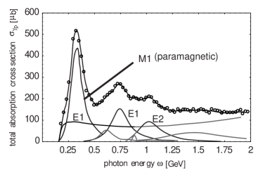
Figure 2: Total photoabsorption cross section decomposed into resonant and nonresonant components [40]. The resonances shown are the $P_{33}(1232)$, $P_{11}(1440)$, $D_{15}(1520)$, $S_{11}(1535)$, $F_{15}(1680)$ and $F_{37}(1950)$. The nonresonant component is of electric dipole $E_{1}$ or $E_{0+}$ multipolarity as shown in the right panel and a mixture of $E1$ and $M1$ multipolarity at higher energies

In addition to the resonances, Figure 2 contains a continuous nonresonant part. This continuous part of the spectrum corresponds to the nonresonant cross section where the low-energy part up to about 500 MeV is mainly given by the $E_{0+}$ electric-dipole (E1) single-pion photoproduction process. There are also minor magnetic-dipole (M1) and mixed M1–E2 single-pion photoproduction processes. At higher energies the photoabsorption cross section is due to two-pion processes which mainly are of the type $\gamma N\to\pi N^{*}\to N\pi\pi$ and, thus combine nonresonant and resonant processes during the absorption.

Though Figure 2 is very useful as an overview [17] for quantitative predictions of partial photoabsorption cross sections information is more appropriate which has been obtained in recent time from the study of photo-meson amplitudes [24]. This will be explained in more detail in subsection 3.3.

3.2 The level scheme of the nucleon

Figure 2 shows only the strongest resonances located below 2 GeV excitation energy. Therefore, it is of interest to present a complete overview over the level scheme for this energy range. Figure 3 shows the level scheme of the nucleon corresponding to the first three HO shells.

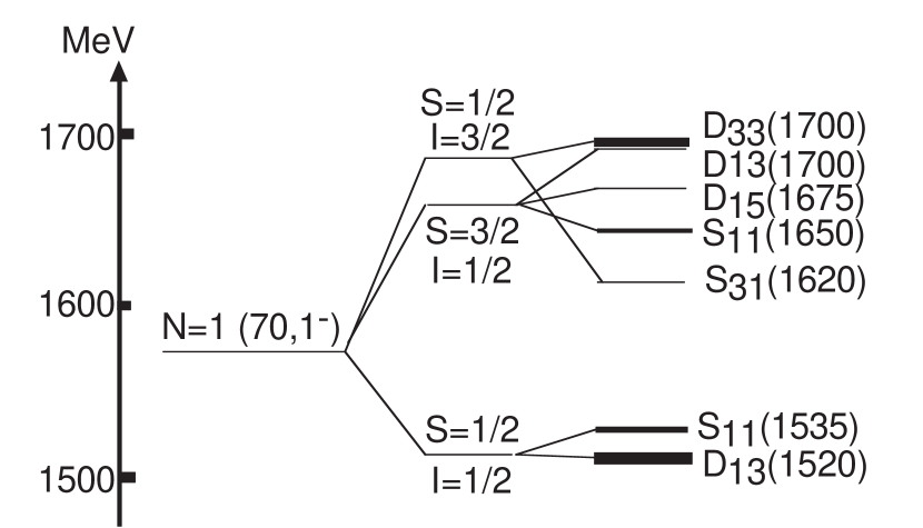
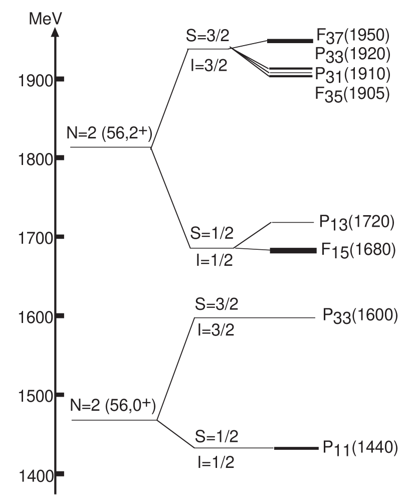
Figure 3: The $N=0$ $(56,0^{+}_{0})$ (left), $N=1$ $(70,1^{-}_{1})$ (middle), and $N=2$ $(56,0^{+}_{2})$, $(56,2^{+}_{2})$ (right) partial level schemes of the nucleon

In total four resonance regions are formed where resonant states with especially large strengths are found. Quantitative information on the strength is given in [20] in terms of integrated photoabsorption cross sections. In Figure 3 the strong states are depicted by thick bars. The first resonance region is solely due to the $P_{33}(1232)$ state which as a $I=3/2$ state is of equal photon-excitation strength for the proton and the neutron. The second resonance region is due to the $D_{13}(1520)$ state and to a lesser extent to the $S_{11}(1535)$ state. The third resonance region consists of the $F_{15}(1680)$ and the $D_{33}(1700)$ states. For the proton the two contributions are of approximately equal strength, whereas for the neutron according to the general rule for $I=1/2$ states based on the quark model the $F_{15}(1680)$ contribution is largely suppressed. The fourth resonance is due to the $F_{37}(1950)$ state which is of equal strength for the proton and the neutron.

3.3 Predicted photoabsorption cross sections

For the prediction of resonant cross sections in principle a direct calculation from the CGLN amplitudes is possible, provided the one-pion branching $\Gamma_{\pi}/\Gamma_{r}$ of the resonances is taken into account where necessary. However, as shown in [20], a much more precise procedure is available. This method makes use of the parameters of the resonances extracted from the CGLN data [24].

For the precise prediction of $\sigma^{n}_{T}=\frac{1}{2}\,(\sigma^{n}_{3/2}+\sigma^{n}_{1/2})$ we use the Walker parameterization of resonant states where the cross sections are represented in terms of Lorentzians in the form

$$I=I_{r}\left(\frac{k_{r}}{k}\right)^{2}\frac{W^{2}_{r}\,\Gamma(q)\Gamma^{*}_{\gamma}(k)}{(W^{2}-W^{2}_{r})^{2}+W^{2}_{r}\,\Gamma^{2}(q)}$$ (47)

where $W_{r}$ is the resonance energy of the resonance. The functions $\Gamma(q)$ and $\Gamma^{*}_{\gamma}(k)$ are chosen such that a precise representation of the shapes of the resonances are obtained. The appropriate parameterizations and the related references are given in [20]. Furthermore, some consideration given in [20] shows that the peak cross section can be expressed through the resonance couplings in the following form

$$I_{r}=\frac{2\,m}{W_{r}\Gamma_{r}}\left[|A_{1/2}|^{2}+|A_{3/2}|^{2}\right].$$ (48)

For the total widths $\Gamma_{r}$ and the resonance couplings precise data are available. Tabulations of values adopted for the present purpose are given in [20].

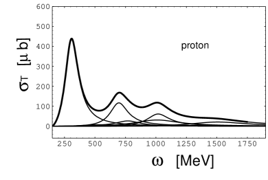
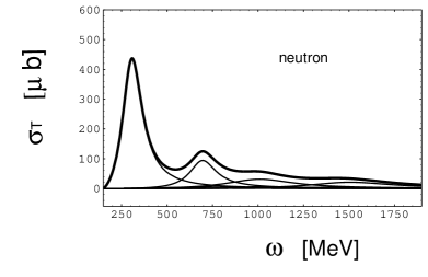
Figure 4: Resonant part of the helicity independent photo-absorption cross section for the proton and the neutron. Thick line: Sum of all resonances. Thin lines: Contributing single resonances. The energies and strengths corresponding to these resonances are given in Tables 7 and 8 of [20].

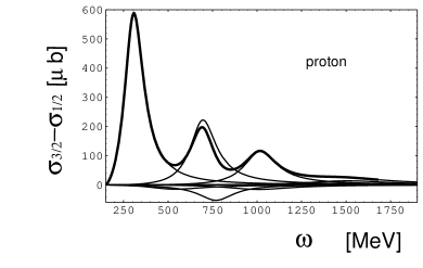
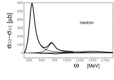
Figure 5: Resonant part of the helicity dependent photo absorption cross section for the proton and the neutron. Thick line: Sum of all resonances. Thin lines: Contributing single resonances. The energies and strengths corresponding to these resonances are given in Tables 7 and 8 of [20]. The signs of the cross sections are given in Table 3 of [20].

The cross-section difference $\sigma_{3/2}-\sigma_{1/2}$ can also be calculated directly from the CGLN amplitudes. But also for this difference we propose a more appropriate procedure. This procedure makes use of the fact that precise values for total cross sections $\sigma_{T}$ are easier to obtain than for the cross section differences $\sigma_{3/2}-\sigma_{1/2}$. Therefore, we start from the relation

$$\sigma^{n}_{3/2}-\sigma^{n}_{1/2}=A_{n}\,\frac{1}{2}\,(\sigma^{n}_{3/2}+\sigma^{n}_{1/2})=A_{n}\,\sigma^{n}_{T}$$ (49)

where $n$ refers to the different resonant states. The results obtained for $\sigma_{T}$ and $\sigma_{3/2}-\sigma_{1/2}$ from the present procedure are shown in Figures 4 and 5. The resonance couplings $A_{3/2}$ and $A_{1/2}$, the widths $\Gamma_{r}$ and the scaling factors $A_{n}$ entering into (49) are tabulated in [20].

In Figure 4 we show the total resonant cross sections for the individual resonances of the proton and the neutron. Four resonance regions are clearly visible in both cases, however with the difference that for the neutron the third resonance region is largely suppressed. This difference may be traced back to the $F_{15}(1680)$ resonance which is smaller by a factor of 10 for the neutron as compared with the proton. Figure 5 shows the corresponding cross section differences $\sigma_{3/2}-\sigma_{1/2}$. Here again the line obtained for the $F_{15}(1680)$ resonance is largely suppressed in case of the neutron.

3.4 Predicted difference of helicity dependent cross sections compared with experimental data

Recent measurements at MAMI (Mainz) and ELSA (Bonn) have led to very valuable data for the helicity dependence of the total photo-absorption cross section of the proton and the neutron [41, 42, 43, 44, 45, 46, 47, 48, 49, 50, 51, 52, 53, 54]. In the following we will compare experimental data obtained for the proton with the predictions of the present approach. We restrict the discussion to the proton because of the higher precision of the experimental data as compared to the neutron.

In Figure 6 we discuss experimental data obtained at MAMI (Mainz). In order to clearly demonstrate the resonant structure of the first and the second resonance we have eliminated the nonresonant contribution from the figure and only keep the resonant contribution. The baseline of the resonant contribution now is the abscissa. Technically this has been achieved by adding the predicted nonresonant contribution to the experimental data. The $P_{33}(1232)$ and $D_{13}(1520)$ resonances make strong positive contributions whereas the $P_{11}(1440)$ and $S_{13}(1535)$ resonances make small negative contributions. During the fitting procedure it was found out that slight shifts of some of the parameters within their margins of errors led to an improvement of the fit to the experimental data. For the $P_{33}(1232)$ resonance these shifts are 1232 MeV $\to$ 1226 MeV for the position

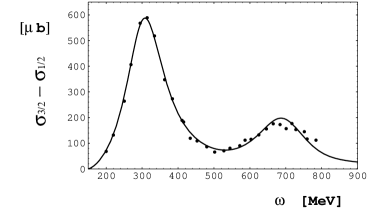
Figure 6: Predicted difference of helicity dependent cross sections for the proton in the first and second resonance region compared with experimental data. The experimental data are taken from [42]. The nonresonant contribution is eliminated from the figure by a procedure described in the text. The contributions shown in the left panel are the resonances $P_{33}(1232)$ (1), $P_{11}(1440)$ (2), $D_{13}(1520)$ (3), and $S_{11}(1535)$ (4).

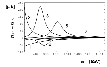
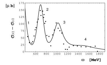
Figure 7: Predicted difference of helicity dependent cross sections for the proton in the second, third and fourth resonance region compared with experimental data. The experimental data are taken from [47]. The contributions shown in the left panel are the tail of the $P_{33}(1232)$ resonance (2), the nonresonant contribution (1), the $P_{11}(1440)$, $D_{13}(1520)$ (3), $S_{11}(1535)$ (4), $S_{11}(1650)$, $D_{15}(1675)$, $F_{15}(1680)$ (5), $D_{33}(1700)$, $F_{35}(1905)$ and $F_{37}(1950)$ (6) resonances. The numbers given in the right panel denote the resonance regions 1–4.

of the peak, 130 MeV $\to$ 120 MeV for the width of the resonance and 1.26 $\to$ 1.36 for the quantity $A_{n}$ defined in Eq. (49). This means that the integrated cross section and also the integrated energy-weighted cross section remain constant. For the $D_{13}(1520)$ resonance the shifts were 1520 $\to$ 1490 for the position of the peak, 120 MeV $\to$ 130 for the width of the resonance. All other parameters remained unmodified compared to the predictions given in [20].

Figure 7 differs from Figure 6 by the fact that the nonresonant contribution is not eliminated from the Figure but included into the theoretical curve. Indeed, the dip between the first and the second resonance shown in the right panel of Figure 7 is strongly influenced by the nonresonant cross sections represented by curve 1 in the left panel. In the left panel only the stronger resonances have been identified through a number, though all the relevant resonances have been shown. As in Figure 6 some shifts of parameters have been tested in order to possibly improve on the fit to the experimental data. The only shift of some relevance was the generation of a small negative contribution from the $D_{33}(1700)$ resonance by shifting the quantity $A_{n}$ from $0$ $\to$ $-0.5$.

The importance of the findings made in Figures 6 and 7 is that our procedure of applying the Walker parameterization to the helicity dependent cross section difference $(\sigma_{3/2}-\sigma_{1/2})$ has been tested and found valid. This makes it possible to apply this procedure also to other problems as there is the prediction and interpretation of the $s$-channel contribution to the forward and backward angle spin-polarizabilities $\gamma_{0}$ and $\gamma_{\pi}$, respectively. Furthermore, we have clearly demonstrated that the upper part of the cross section in the right panel of Figure 7 is due to the $F_{37}(1950)$ resonance as anticipated before [47].

3.5 Nonresonant excitation of the nucleon

Figure 8: Photoabsorption cross section $\sigma(E_{0+})$ due to $s$-wave single pion photoproduction for the proton (p) and the neutron (n). The two upper curves have been calculated in Born approximation. The two lower curves are empirical results [55, 56, 24] and extrapolations between 500 and 700 MeV

In Figure 8 the experimental $E_{0+}$ cross section is shown together with the prediction obtained in the Born approximation. We see that in both cases the cross sections for the neutron are larger than the cross sections for the proton. For the Born approximation this has been discussed in the textbook of Ericson and Weise (see p. 286 of [57]). The explanation is that for meson photoproduction the electric dipole amplitude $E_{0+}$ is larger for the reaction $\gamma n\to\pi^{-}p$ than for the reaction $\gamma p\to\pi^{+}n$ because of the larger electric dipole moment in the final state. Indeed the ratio of the two cross sections given for the Born approximation can be obtained from ratio of the $\pi^{-}p$ and $\pi^{+}n$ dipole moments. The difference in dipole moments which also shows up in the empirical $E_{0+}$ cross sections leads to an explanation for the fact that the neutron has a larger electric polarizability than the proton. The empirical cross section shown in Figure 8 above $\omega=500$ MeV are extrapolations of data given in [55, 56, 24]. The extrapolation was necessary because this cross section is purely nonresonant only up to $\omega=500$ MeV. Above this energy the interference of cross sections from nucleon resonances is observed. The guidance for the extrapolation is taken from the Born approximation showing that the cross section is almost a straight line at energies above 450 MeV.

3.6 Diagrammatic representation of Compton scattering

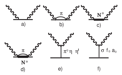
Figure 9: Graphs of nucleon Compton scattering. a) Born term, b) single-pion photoproduction, c) resonant excitation of the nucleon and d) two-pion photoproduction. The crossed graphs accompanying the graphs a) to d) are not shown. The $t$-channel graphs in e) and f) correspond to pointlike singularities due to the pseudoscalar meson $\pi^{0}$, $\eta$ and $\eta^{\prime}$ and the scalar mesons $\sigma(600)$, $f_{0}(980)$ and $a_{0}(980)$. These graphs are shown for illustration whereas quantitative predictions are based on dispersion theory.

The method of predicting polarizabilities is based on dispersion theory applied to partial photoabsorption cross-sections. Nevertheless, it is of interest for illustration to show the Compton scattering process in terms of diagrams as carried out in Figure 9. We see that in addition to the nonresonant single-pion channel (b) and the resonant channel (c) we have three further contributions. Graph (d) corresponds to Compton scattering via the transition $\gamma N\to\Delta\pi$ to the intermediate state. This represents the main component of those photomeson processes where two pions are in the final state. Graph e) is the well-known pseudoscalar $t$-channel graph where in addition to the dominant $\pi^{0}$ pole contribution also the small contributions due to $\eta$ and $\eta^{\prime}$ mesons are taken into account. Graph f) depicts the scalar counterpart of the pseudoscalar pole term e). At first sight these scalar pole-terms appear inappropriate because the scalar particles and especially the $\sigma$ meson have a large width when observed on shell. However, this consideration overlooks that in a Compton scattering process the scalar particles are intermediate states of the scattering process where the broadening due to the $\pi\pi$ final state is not effective. This leads to the conclusion that the scalar pole terms indeed provide the correct description of the scattering process. Further information is given in subsection 5.4.

3.7 Predicted polarizabilities obtained for the $s$-channel

Using the sum rules given in Eqs. (25) to (37) and applying them to the photoabsorption cross sections given in subsections 3.3 to 3.5 the polarizabilities and spin-polarizabilities given in Table 2 are obtained. Lines 2-12 contain the contributions of the nucleon resonances, with the sum of the resonant contributions given in line 13. The nonresonant electric and magnetic single-pion contributions are given in lines 14-16, and the contribution due to the two-pion channel in line 17. Line 18 contains the total $s$-channel contribution.

Table 2: Resonant (lines 2–12), single-pion nonresonant (lines 14–16) and two-pion (line 17) components of the polarizabilities. Line 13 contains the total resonant components and line 18 the total $s$-channel component. The electric and magnetic polarizabilities are in units of $10^{-4}$fm³, the spin polarizabilities in units of $10^{-4}$fm⁴.

	$\alpha_{p}$	$\beta_{p}$	$\alpha_{n}$	$\beta_{n}$	$\gamma^{(p)}_{0}$	$\gamma^{(n)}_{0}$	$\gamma^{(p)}_{\pi}$	$\gamma^{(n)}_{\pi}$
$P_{33}(1232)$	$-1.07$	$+8.32$	$-1.07$	$+8.32$	$-3.03$	$-3.03$	$+5.11$	$+5.11$
$P_{11}(1440)$	$-0.02$	$+0.14$	$-0.01$	$+0.05$	$+0.05$	$+0.02$	$-0.10$	$-0.04$
$D_{13}(1520)$	$+0.68$	$-0.16$	$+0.55$	$-0.13$	$-0.14$	$-0.07$	$-0.39$	$-0.20$
$S_{11}(1535)$	$+0.21$	$-0.05$	$+0.06$	$-0.01$	$+0.05$	$+0.01$	$+0.13$	$+0.04$
$S_{11}(1650)$	$+0.05$	$-0.01$	$+0.00$	$-0.00$	$+0.01$	$+0.00$	$+0.03$	$+0.00$
$D_{15}(1675)$	$+0.01$	$-0.00$	$+0.08$	$-0.02$	$-0.00$	$-0.00$	$-0.00$	$-0.01$
$F_{15}(1680)$	$-0.07$	$+0.25$	$-0.01$	$+0.03$	$-0.02$	$-0.00$	$+0.13$	$+0.01$
$D_{33}(1700)$	$+0.25$	$-0.07$	$+0.25$	$-0.07$			$-0.00$	$-0.00$
$F_{35}(1905)$	$-0.01$	$+0.02$	$-0.01$	$+0.02$			$+0.01$	$+0.01$
$P_{33}(1920)$	$-0.01$	$+0.02$	$-0.01$	$+0.02$			$+0.01$	$+0.01$
$F_{37}(1950)$	$-0.03$	$+0.10$	$-0.03$	$+0.10$			$+0.01$	$+0.01$
sum-res.	$-0.01$	$+8.56$	$-0.20$	$+8.31$	$-3.08$	$-3.07$	$+4.94$	$+4.94$
$E_{0+}$	$+3.19$	$-0.34$	$+4.07$	$-0.43$	$+2.47$	$+3.18$	$+3.75$	$+4.81$
$M^{(3/2)}_{1-}$	$-0.04$	$+0.35$	$-0.04$	$+0.35$	$-0.11$	$-0.11$	$-0.18$	$-0.18$
$(M,E)^{(1/2)}_{1+}$	$-0.06$	$+0.47$	$-0.21$	$+1.44$	$+0.14$	$+0.38$	$+0.24$	$+0.66$
$\gamma N\to\pi\Delta$	$+1.4$	$+0.4$	$+1.5$	$+0.4$	$\,\,\,\,\,0.00$	$\,\,\,\,\,0.00$	$-0.28$	$-0.23$
$s$-channel	$+4.48$	$+9.44$	$+5.12$	$+10.07$	$-0.58$	$+0.38$	$+8.47$	$+10.00$

The forward-angle spin-polarizabilities have the peculiarity that the proton and neutron values have different signs and both are very close to zero. Therefore these values should be given with an error. Taking into account the well known rules of error analysis one obtains

$$\gamma^{(p)}_{0}=-0.58\pm 0.20,\quad\gamma^{(n)}_{0}=+0.38\pm 0.22.$$ (50)

For the proton the present result may be compared with the most recent previous evaluation [58]. The main result of this evaluation is $\gamma^{(p)}_{0}=-0.90\pm 0.08\pm 0.11$. Other results based on different photomeson analyses are $\gamma^{(p)}_{0}=-0.67$ (HDT), $-0.65$ (MAID), $-0.86$ (SAID) and $-0.76$ (DMT). In view of the fact that different data sets have been used in these analyses the consistency of these results and the agreement with our result appears remarkably good. A comparison is also possible with the analysis of Drechsel et al. [59] based on CGLN amplitudes and dispersion theory. The numbers obtained are $\gamma^{(p)}_{0}=-0.6$ and $\gamma^{(n)}_{0}=+0.0$ based on the HDT parameterization. The result obtained in [59] for the proton is in close agreement with our result. The result obtained in [59] for the neutron confirms our prediction that the quantity $\gamma^{(n)}_{0}$ has the tendency of being shifted towards positive values. In [59] also a detailed comparison with chiral perturbation theory is given which should not be repeated here.

4 S-matrix and invariant amplitudes

For the following part of the present paper it is necessary to outline the theoretical tools on a wider basis. These tools are the S-matrix for nucleon Compton scattering and the invariant amplitudes.

4.1 S-matrix

The amplitude $T_{fi}$ for Compton scattering

$$\gamma(k)N(p)\to\gamma^{\prime}(k^{\prime})N(p^{\prime})$$ (51)

is related to the $S$-matrix of the reaction through the relation

$$\langle f|S-1|i\rangle=i(2\pi)^{4}\delta^{4}(k+p-k^{\prime}-p^{\prime})T_{fi}.$$ (52)

The quantities $k=(\omega,{\bf k})$, $k^{\prime}=(\omega^{\prime},{\bf k}^{\prime})$, $p=(E,{\bf p})$, $p^{\prime}=(E^{\prime},{\bf p^{\prime}})$ are the four momenta of the photon and the nucleon in the initial and final states, respectively, related to the Mandelstam variables via

$$s=(k+p)^{2},\quad t=(k-k^{\prime})^{2},\quad u=(k-p^{\prime})^{2}.$$ (53)

The scattering amplitude $T_{fi}$ may be expressed on an orthogonal basis suggested by Prange [60] by means of six invariant amplitudes $T_{k}(\nu,t)$ leading to the general form [34]

$$T_{fi} =\bar{u^{\prime}}e^{\prime}{}^{*\mu}\Big{[}-\frac{P^{\prime}_{\mu}P^{\prime}_{\nu}}{P^{\prime}{}^{2}}(T_{1}+(\gamma\cdot K)T_{2})-\frac{N_{\mu}N_{\nu}}{N^{2}}(T_{3}+(\gamma\cdot K)T_{4})$$ (54)

$$+i\frac{P^{\prime}_{\mu}N_{\nu}-P^{\prime}_{\nu}N_{\mu}}{P^{\prime}{}^{2}K^{2}}\gamma_{5}T_{5}+i\frac{P^{\prime}_{\mu}N_{\nu}+P^{\prime}_{\nu}N_{\mu}}{P^{\prime 2}K^{2}}\gamma_{5}(\gamma\cdot K)T_{6}\Big{]}e^{\nu}u.$$

In (54) $u^{\prime}$ and $u$ are the Dirac spinors of the final and the initial nucleon, $e^{\prime}$ and $e$  are the polarization 4-vectors of the final and the initial photon, and $\gamma_{5}=-i\gamma_{0}\gamma_{1}\gamma_{2}\gamma_{3}$. The 4-vectors $P^{\prime}$, $K$ and $N$ together with the vector $Q$ are orthogonal and are expressed in terms of the 4-momenta $p^{\prime}$, $k^{\prime}$ and $p$, $k$ of the final and initial nucleon and photon, respectively, by

$$K=\frac{1}{2}(k+k^{\prime}),\quad P^{\prime}=P-\frac{K(P\cdot K)}{K^{2}},\quad N_{\mu}=\epsilon_{\mu\nu\lambda\sigma} P^{\prime}{}^{\nu}Q^{\lambda}K^{\sigma},$$

$$P=\frac{1}{2}(p+p^{\prime}),\quad Q=\frac{1}{2}(k^{\prime}-k)=\frac{1}{2}(p-p^{\prime})$$ (55)

where $\epsilon_{\mu\nu\lambda\sigma}$ is the antisymmetric tensor with $\epsilon_{0123}=1$. The amplitudes $T_{k}$ are functions of the two variables $\nu$ and $t$ with

$$\nu=\frac{s-m^{2}+t/2}{2m}$$ (56)

and $m$ is the mass of the nucleon. The normalization of the amplitude $T_{fi}$ is determined by

$$\bar{u}u=2m,\quad\frac{d\sigma}{d\Omega}=\frac{1}{64\pi^{2}s}\sum_{\rm spins}|T_{fi}|^{2}.$$ (57)

It follows from crossing symmetry of $T_{fi}$, that $T_{1,3,5,6}$ and $T_{2,4}$ are even and odd functions of $\nu$, respectively.

The amplitudes $T_{k}(\nu,t)$ do not have kinematic singularities, but there are kinematic constraints, which arise from the vanishing of $P^{\prime}{}^{2}$, $N^{2}$ and $P^{\prime}{}^{2}K^{2}$ in the dominators of the decomposition (54) at certain values of $\nu$ and $t$. The kinematic constraints can be removed by introducing linear combinations of the amplitudes $T_{k}(\nu,t)$. This problem has first been satisfactorily solved by Bardeen and Tung [61]. However, the Bardeen and Tung amplitudes contain the inconvenience that part of them are even functions of $\nu$ and part of them odd functions. This inconvenience has been removed by L’vov [62] so that these latter amplitudes now have become standard.

4.2 Invariant amplitudes

The linear combinations introduced by L’vov [62] are

$$A_{1}=\frac{1}{t}[T_{1}+T_{3}+\nu(T_{2}+T_{4})],$$

$$A_{2}=\frac{1}{t}[2T_{5}+\nu(T_{2}+T_{4})],$$

$$A_{3}=\frac{m^{2}}{m^{4}-su}\left[T_{1}-T_{3}-\frac{t}{4\nu}(T_{2}-T_{4})\right],$$

$$A_{4}=\frac{m^{2}}{m^{4}-su}\left[2mT_{6}-\frac{t}{4\nu}(T_{2}-T_{4})\right],$$

$$A_{5}=\frac{1}{4\nu}[T_{2}+T_{4}],$$

$$A_{6}=\frac{1}{4\nu}[T_{2}-T_{4}].$$ (58)

The amplitudes $A_{i}(\nu,t)$ are even functions of $\nu$ and have no kinematic singularities or kinematic constraints. They have poles at zero energy because of contributions of the nucleon in the intermediate state. These poles are contained in two Born diagrams with the pole propagator $(\gamma\cdot p-m)^{-1}$ and on-shell vertices $\Gamma_{\mu}(p+k,p)=\gamma_{\mu}+[\gamma\cdot k,\gamma_{\mu}]\kappa/4m$, where $\kappa=1.793q-1.913(1-q)$ is the nucleon anomalous magnetic moment. Here the electric charge of the nucleon, $q=\frac{1}{2}(1+\tau_{3})=1$ or $0$ is introduced. The Born contributions to the amplitudes $A_{i}$ have a pure pole form

$$A^{\rm B}_{i}(\nu,t)=\frac{me^{2}r_{i}(t)}{(s-m^{2})(u-m^{2})},$$ (59)

where e is the elementary electric charge ($e^{2}/4\pi=1/137.04$) and

$$r_{1}=-2q^{2}+(\kappa^{2}+2q\kappa)\frac{t}{4m^{2}},\quad r_{2}=2q\kappa+2q^{2}+(\kappa^{2}+2q\kappa)\frac{t}{4m^{2}},$$

$$r_{3}=r_{5}=\kappa^{2}+2q\kappa,\quad r_{4}=\kappa^{2},\quad r_{6}=-\kappa^{2}-2q\kappa-2q^{2}.$$ (60)

4.3 Lorentz invariant definition of polarizabilities

The relations between the amplitudes $f$ and $g$ introduced in Section 2.1 and the invariant amplitudes $A_{i}$ [35, 34] are

$$f_{0}(\omega)=-\frac{\omega^{2}}{2\pi}\left[A_{3}(\nu,t)+A_{6}(\nu,t)\right],\quad\quad\quad g_{0}(\omega)=\frac{\omega^{3}}{2\pi m}A_{4}(\nu,t),$$ (61)

$$f_{\pi}(\omega)=-\frac{\omega\omega^{\prime}}{2\pi}\left(1+\frac{\omega\omega^{\prime}}{m^{2}}\right)^{1/2}\left[A_{1}(\nu,t)-\frac{t}{4m^{2}}A_{5}(\nu,t)\right],$$ (62)

$$g_{\pi}(\omega)=-\frac{\omega\omega^{\prime}}{2\pi m}\sqrt{\omega\omega^{\prime}}\left[A_{2}(\nu,t)+\left(1-\frac{t}{4m^{2}}\right)A_{5}(\nu,t)\right],$$ (63)

$$\omega^{\prime}(\theta=\pi)=\frac{\omega}{1+2\frac{\omega}{m}},\,\,\nu=\frac{1}{2}(\omega+\omega^{\prime}),\,\,t(\theta=0)=0,\,\,t(\theta=\pi)=-4\omega\omega.^{\prime}$$ (64)

For the electric, $\alpha$, and magnetic, $\beta$, polarizabilities and the spin polarizabilities $\gamma_{0}$ and $\gamma_{\pi}$ for the forward and backward directions, respectively, we obtain the relations

$$\alpha+\beta=-\frac{1}{2\pi}\left[A^{\rm nB}_{3}(0,0)+A^{\rm nB}_{6}(0,0)\right],\quad\alpha-\beta=-\frac{1}{2\pi}\left[A^{\rm nB}_{1}(0,0)\right],$$

$$\gamma_{0}=\frac{1}{2\pi m}\left[A^{\rm nB}_{4}(0,0)\right],\quad\quad\quad\quad\quad\quad\quad\,\,\,\gamma_{\pi}=-\frac{1}{2\pi m}\left[A^{\rm nB}_{2}(0,0)+A^{\rm nB}_{5}(0,0)\right],$$ (65)

showing that the invariant amplitudes may be understood as a generalization of the polarizabilities.

According to Eqs. (61) to (65) the following linear combinations of invariant amplitudes are of special importance because they contain the physics of the four fundamental sum rules,  viz. the BEFT (66), LN (67), BL (68) and GDH (69) sum rules, respectively:

$${\tilde{A}}_{1}(\nu,t)\equiv A_{1}(\nu,t)-\frac{t}{4m^{2}}A_{5}(\nu,t),$$ (66)

$${\tilde{A}}_{2}(\nu,t)\equiv A_{2}(\nu,t)+\left(1-\frac{t}{4m^{2}}\right)A_{5}(\nu,t),$$ (67)

$${\tilde{A}}_{3}(\nu,t)\equiv A_{3+6}(\nu,t)\equiv A_{3}(\nu,t)+A_{6}(\nu,t),$$ (68)

$${\tilde{A}}_{4}(\nu,t)\equiv A_{4}(\nu,t).$$ (69)

5 From the Bernabeu-Ericson-FerroFontan-Tarrach (BEFT) sum rule to the $\sigma$-meson pole

The introduction of the $\sigma$-meson pole dates back to the seminal paper of L’vov et al. [34], where for the first time a precise prediction of Compton differential cross sections in the second resonance region of the proton for a large angular interval was achieved The observation made in these investigations was that at high energies and large scattering angles the prediction of Compton differential cross sections requires a large contribution from the scalar $t$-channel. In [34] it was empirically shown that this contribution can be represented by a $\sigma$-meson pole with a real mass $m_{\sigma}$ of about 600 MeV in complete analogy to the $\pi^{0}$-meson pole. However, there remained an important difference between the two poles, because the $\pi^{0}$-meson pole had a firm theoretical justification, whereas the $\sigma$-meson pole was considered as a tool of computation without a good theoretical basis. The reason was that in reactions like $\gamma\gamma\to\sigma\to\pi\pi$ the $\sigma$-meson is represented by a pole with a complex mass $\sqrt{s_{\sigma}}=M_{\sigma}-i\,\frac{1}{2}\Gamma_{\sigma}$ located on the second Riemann sheet. This fact seems to contradict the assumption of a pole located on the real $s$-axis.

An essential step forward was made in [16] where it was shown that the use of arguments contained in the work of Scadron et al. [29] leads to a firm justification of the $\sigma$-pole ansatz and to a quantitative prediction of $(\alpha-\beta)^{t}$ and $m_{\sigma}$. The corresponding chain of arguments are outlined in the following.

5.1 The BEFT sum rule

The BEFT sum rule [25, 26, 63, 64, 65, 66] may be derived from the non-Born part of the invariant amplitude (see [34, 1])

$${\tilde{A}}_{1}(s,u,t)\equiv A_{1}(s,u,t)-\frac{t}{4m^{2}}A_{5}(s,u,t)$$ (70)

by applying the fixed-$\theta$ dispersion relation for $\theta=180^{\circ}$. Then we arrive at

$${\rm Re}{\tilde{A}}^{\rm nB}_{1}(s,u,t) = \frac{1}{\pi}{\cal P}\int^{\infty}_{s_{0}}\left(\frac{1}{s^{\prime}-s}+\frac{1}{s^{\prime}-u}-\frac{1}{s^{\prime}}\right){\rm Im}_{s}{\tilde{A}}_{1}(s^{\prime},u^{\prime},t^{\prime})ds^{\prime}$$ (71)

$$+ \frac{1}{\pi}{\cal P}\int^{\infty}_{t_{0}}{\rm Im}_{t}{\tilde{A}}_{1}(s^{\prime},u^{\prime},t^{\prime})\frac{dt^{\prime}}{t^{\prime}-t}\,\,,$$

where $s_{0}=(m+m_{\pi})^{2}$, $t_{0}=4m^{2}_{\pi}$, $s^{\prime}+u^{\prime}+t^{\prime}=2m^{2}$ and $s^{\prime}u^{\prime}=m^{4}$. Using

$$\alpha-\beta=-\frac{1}{2\pi}{\tilde{A}}^{\rm nB}_{1}(m^{2},m^{2},0)=(\alpha-\beta)^{s}+(\alpha-\beta)^{t}$$ (72)

we arrive at

$$(\alpha-\beta)^{s}=-\frac{1}{2\pi^{2}}\int^{\infty}_{s_{0}}\frac{s^{\prime}+m^{2}}{s^{\prime}-m^{2}}{\rm Im}_{s}{\tilde{A}}_{1}(s^{\prime},u^{\prime},t^{\prime})\frac{ds^{\prime}}{s^{\prime}}\,\,,$$ (73)

$$(\alpha-\beta)^{t}=-\frac{1}{2\pi^{2}}\int^{\infty}_{t_{0}}{\rm Im}_{t}{\tilde{A}}_{1}(s^{\prime},u^{\prime},t^{\prime})\frac{dt^{\prime}}{t^{\prime}}.$$ (74)

5.1.1 The $s$-channel part of the BEFT sum rule

Using Eq. (73) and the relation for ${\rm Im}f_{\pi}$ derived in Eq. (15) we arrive at the $s$-channel part of the BEFT sum rule given in Eq. (27). The main contribution to $(\alpha-\beta)^{s}$ comes from the photoproduction of $\pi N$ states. For these states, the cross-section difference can be expressed in terms of the standard CGLN amplitudes via

$$\left[\sigma(\omega,\Delta P={\rm yes})-\sigma(\omega,\Delta P={\rm no})\right]^{\pi N}=4\pi\frac{q}{k}\sum^{\infty}_{k=0}(-1)^{k}(k+1)^{2}$$

$$\hskip 56.9055pt\times\Big{\{}(k+2)\left(|E_{k+}|^{2}-|M_{(k+1)-}|^{2}\right)+k\left(|M_{k+}|^{2}-|E_{(k+1)-}|^{2}\right)\Big{\}}^{\pi N},$$ (75)

where $q=|{\bf q}|$ and $k=|{\bf k}|$ are the pion and photon momenta in the cm system, respectively.

In (75) the quantity $\left[\sigma(\omega,\Delta P={\rm yes})-\sigma(\omega,\Delta P={\rm no})\right]$ is expressed in terms of CGLN amplitudes which where barely known when the first studies of the BEFT sum rule where carried out and remained of limited precision later on. A great improvement was possible in the present investigation where the difference $\left[\sigma(\omega,\Delta P={\rm yes})-\sigma(\omega,\Delta P={\rm no})\right]$ is calculated from partial cross sections as described in section 3.

5.1.2 The $t$-channel part of the BEFT sum rule

The imaginary part of the amplitude ${\tilde{A}}_{1}$ (Eq. 70) in the $t$-channel can be found using the general unitarity relation

$${\rm Im}_{t}T(\gamma\gamma\to N{\bar{N}})=\frac{1}{2}\sum_{n}(2\pi)^{4}\delta^{4}(P_{n}-P_{i})T(\gamma\gamma\to n)T^{*}(N{\bar{N}}\to n),$$ (76)

where the sum on the right-hand side is taken over all allowed intermediate states $n$ having the same total 4-momentum as the initial state. In the following we restrict ourselves to two-pion intermediate states, i.e. $n=\pi\pi$.

The amplitudes $T(\gamma\gamma\to\pi\pi)$ and $T(\pi\pi\to\bar{N}N)$ are constructed by making use of available experimental information on two different reactions. For the amplitude $T(\gamma\gamma\to\pi\pi)$ this is the two-photon fusion reaction $\gamma\gamma\to\pi\pi$. Since there are no data on the reaction $\pi\pi\to\bar{N}N$, the amplitude $T(\pi\pi\to\bar{N}N)$ is constructed in a dispersive approach using the well known amplitudes of the pion-nucleon scattering reaction $\pi N\to N\pi$. At $t>m^{2}_{\pi}$ unitarity shows that the phases of the amplitudes $T(\gamma\gamma\to\pi\pi)$ and $T(\pi\pi\to\bar{N}N)$ are the same and equal to the phases of pion-pion scattering, $\delta^{J}_{I}$, which are known from the data on the reaction $\pi p\to p\pi\pi$.

The phase-dependent factor entering into the amplitude of a narrow resonance is described by a Breit-Wigner curve, whereas for the present case of a very broad resonance as given by the functions $\delta^{J}_{I}(t)$, a generalized version of the Breit-Wigner curve has to be used. This generalized phase-dependent factor is given by the Omnès [67] function $\Omega^{J}_{I}(t)$ defined through

$$\Omega^{J}_{I}(t)={\rm exp}{\left[\frac{t}{\pi}\int^{\infty}_{4m^{2}_{\pi}}dt^{\prime}\frac{\delta^{J}_{I}(t^{\prime})}{t^{\prime}(t^{\prime}-t-i0)}\right]}\equiv e^{i\delta^{J}_{I}(t)}{\rm exp}{\left[\frac{t}{\pi}{\cal P}\int^{\infty}_{4m^{2}_{\pi}}\frac{\delta^{J}_{I}(t^{\prime})dt^{\prime}}{t^{\prime}(t^{\prime}-t)}\right]}.$$ (77)

For the discussion of the properties of the $T(\pi\pi\to\bar{N}N)$ amplitude in the unphysical region $4m^{2}_{\pi}\leq t\leq 4M^{4}$ we use the backward amplitude $F^{(+)}(t)$ discussed by Bohannon [68]. For the pion scattering process the quantity $t$ is negative, whereas for positive $t$ the analytic continuation of $F^{(+)}(t)$ describes the $N\bar{N}\to\pi\pi$ annihilation process for the case that the helicities of the nucleon and the antinucleon are the same, $\lambda=\bar{\lambda}$. This provides us with a tool to construct the $N\bar{N}\to\pi\pi$ amplitude from the measured $\pi N\to\pi N$ amplitude. Since the backward $\pi N\to N\pi$ scattering amplitude implies also backward $N\bar{N}\to\pi\pi$ annihilation, it can be shown that the first two terms of the expansion for $F^{(+)}(t)$ at positive $t$ are

$$F^{(+)}(t)=\frac{16\pi}{m(4m^{2}-t)}f^{0}_{+}(t)-\frac{5\pi(t-4m^{2}_{\pi})}{m}f^{2}_{+}(t).$$ (78)

The amplitudes $f^{J}_{+}(t)$ are the partial wave amplitudes introduced by Frazer and Fulco [69], where $J$ denotes the angular momentum of the $\pi\pi$ intermediate state. The $+$ sign denotes that the two helicities $\lambda$ and $\bar{\lambda}$ of $N$ and $\bar{N}$, respectively, are the same, $\lambda=\bar{\lambda}$.

The construction of both amplitudes, $T(\gamma\gamma\to\pi\pi)$ and $T(\pi\pi\to\bar{N}N)$, in connection with the scalar-isoscalar $t$-channel of Compton scattering has first been described and worked out in some detail by Köberle [28] and later discussed by several authors, of whom we wish to cite [70, 66, 56, 7, 71]. For a very broad resonance the appropriate ansatz reads

$$F^{J}_{I\lambda}(t)=\Omega^{J}_{I}(t)P^{J}_{I\lambda}(t).$$ (79)

where $P^{J}_{I\lambda}(t)$ is a real amplitude in the $\gamma\gamma\to\pi\pi$ physical region and $\Omega^{J}_{I}(t)$ the phase-dependent Omnés function discussed above. In (79) $I$ is the isospin of the transition, $J$ the angular momentum and $\lambda\equiv\Lambda^{t}_{\gamma\gamma}$ the helicity difference of the two photons. In the present case we have $\lambda\equiv\Lambda^{t}_{\gamma\gamma}\equiv 0$, so that we can omit the index $\lambda$ without loss of generality. The amplitudes $F^{J}_{I}(t)$ have to be constructed such that they have the correct low-energy properties, reproduce the cross section of the photon fusion reaction $\gamma\gamma\to\pi\pi$ and incorporate the phases $\delta^{J}_{I}(t)$ [72, 73, 74, 75, 76]. For $J=0$ the following form of Eq. (79) has been obtained [71]:

$$F^{0}_{I}(t) = \Omega^{0}_{I}(t)\Big{\{}\left[F^{B,0}_{I}(t)+\Delta F^{0}_{I}(t)\right]{\rm Re}\frac{1}{\Omega^{0}_{I}(t)}-\frac{t^{2}}{\pi}\Big{[}{\cal P}\int^{\infty}_{4m^{2}_{\pi}}[F^{B,0}_{I}(t^{\prime})+\Delta F^{0}_{I}(t^{\prime})]{\rm Im}\frac{1}{\Omega^{0}_{I}(t^{\prime})}\frac{dt^{\prime}}{t^{\prime 2}(t^{\prime}-t)}$$ (80)

$$+ A^{0}_{I}+tB^{0}_{I}\Big{]}\Big{\}}.$$

The expression in Eq. (80) is given for the $s$-wave amplitude where contributions going beyond the Born approximation have been taken into account. The leading term in (80) is a superposition of a Born term, $F^{B,0}_{I}(t)$, and a pion-structure dependent correction, $\Delta F^{0}_{I}(t)$. Since the reactions $\gamma\gamma\to\pi^{+}\pi^{-},\pi^{-}\pi^{+},\pi^{0}\pi^{0}$ show up with two components having isospin $I=2$ and one component having $I=0$ we have to take into account these two isospins with the appropriate weights (for details see [1]).

The amplitudes of interest for the prediction of $(\alpha-\beta)^{t}$ are the $S$-wave amplitude $F^{0}_{0}(t)$ and the $D$-wave amplitude $F^{2}_{0}(t)$ with the $D$-wave amplitude leading to only a small correction. It, therefore, is appropriate to restrict the discussion mainly to the amplitude $F^{0}_{0}(t)$. The essential property of this amplitude is provided by the Omnès function which introduces a zero crossing of the amplitude at about 570 MeV. This zero crossing may be considered as a manifestation of the $\sigma$ meson which shows up through the phase-shift $\delta^{0}_{0}(t)$ of the correlated $\pi\pi$ pair.

If we restrict ourselves in the calculation of the $t$-channel absorptive part to intermediate states with two pions with angular momentum $J\leq 2$, the sum rule (74) takes the convenient form for calculations [26]:

$$(\alpha-\beta)^{t} = \frac{1}{16\pi^{2}}\int^{\infty}_{4m^{2}_{\pi}}\frac{dt}{t^{2}}\frac{16}{4m^{2}-t}\left(\frac{t-4m^{2}_{\pi}}{t}\right)^{1/2}\Big{[}f^{0}_{+}(t)F^{0*}_{0}(t)$$ (81)

$$-\left(m^{2}-\frac{t}{4}\right)\left(\frac{t}{4}-m^{2}_{\pi}\right)f^{2}_{+}(t)F^{2*}_{0}(t)\Big{]},$$

where $f^{(0,2)}_{+}(t)$ and $F^{(0,2)}_{0}(t)$ are the partial-wave helicity amplitudes of the processes $N\bar{N}\to\pi\pi$ and $\pi\pi\to\gamma\gamma$ with angular momentum $J=0$ and $2$, respectively, and isospin $I=0$.

5.2 Test of the BEFT sum rule

Though being the first who published the BEFT sum rule in its presently accepted form, Bernabeu and Tarrach [26] were not aware of the appropriate amplitudes to calculate this sum rule numerically. Also the first calculation of Guiasu and Radescu [63] remained incomplete because the amplitudes were used in the form of their Born approximation and, as the major drawback, the correlation of pions was not taken into account. Table 3 summarizes those results

Table 3: Numerical evaluation of the BEFT sum rule, with corrections a) and b) supplemented by the present author. The unit is $10^{-4}{\rm fm}^{3}$.

$(\alpha_{p}-\beta_{p})^{s}$	$(\alpha_{p}-\beta_{p})^{t}$	$(\alpha_{p}-\beta_{p})$	authors
$-$4.92	+9.28a)	+4.36	Guiasu, Radescu,1978 [64]
$-$4	+10.4b)	+6.4	Budnev, Karnakov, 1979 [65]
$-$5.42	+8.6	$+(3.2^{+2.4}_{-3.6})$	Holstein,Nathan,1994[66]
$-$5.56	+16.46	+(10.7$\pm$0.2)c)	Drechsel,Pasquini, Vanderhaeghen,2003[7]
$-(5.0\pm 1.0)$	$+(14.0\pm 2.0)$	$+(9.0\pm 2.2)$	Levchuk, 2004 [71]
$-4.96$	$+15.0^{d)}$	$+10.0$	present prediction
		$+10.1\pm 0.8$	experiment

a) corrected for the $D$-wave contribution $(-1.7)$ included. In an earlier work Guiasu and Radescu [63] used the Born approximation without $\pi\pi$ correlation for both amplitudes $N\bar{N}\to\pi\pi$ and $\pi\pi\to\gamma\gamma$ and arrived at $(\alpha-\beta)^{t}=+17.51$.
b) correction for the polarizability of the pion (+3.0) included.
c) best value from a range of results given by the authors [7].
d) $\sigma$-pole contribution.

of tests of the BEFT sum rule where at least the $\pi\pi$ correlation is taken into account. In the early works of Guiasu and Radescu [64] and Budnev and Karnakov [65] some missing pieces in the results were identified which are supplemented in Table 3 on the basis of the results given by Holstein and Nathan [66]. In case of the Holstein and Nathan result [66] we interpret the rather conservatively estimated upper and lower bounds as errors. In case of the Drechsel et al. result [7] we quote the $s$-channel and $t$-channel contributions calculated at $\theta=180^{\circ}$. The total result $(\alpha_{p}-\beta_{p})$ is the best value for this quantity extracted by the authors from results obtained in the angular region $140^{\circ}\leq\theta_{\rm lab}\leq 180^{\circ}$.

As will be shown in the following the present prediction given in line 7 of Table 3 is much more precise than the previous predictions given in line 2–6. The reason is that the rather complicated evaluation of the BEFT sum rule is replaced by the straightforward evaluation of the well founded $\sigma$-meson pole. Furthermore, it will be shown that the $\sigma$-meson pole has a transparent interpretation in terms of chiral symmetry breaking. The $(\mbox{\boldmath$\pi$},\sigma)$ quartet may be considered as part of the mesonic structure of the constituent quark. Of these mesons the $(\pi^{0},\sigma)$ doublet has the capability of interacting with two photons and, therefore, to contribute to nucleon Compton scattering and the polarizabilities.

5.3 Comparison of the BEFT sum rule and the $\sigma$ meson pole

The $\pi^{0}$ singularity enters into the invariant amplitude $A_{2}$ and the $\sigma$ singularity into the invariant amplitude $A_{1}$ [34]. Starting this section with the discussion of the properties of the $\pi^{0}$-meson pole we may write down

$${\rm Im}_{t}A^{\pi^{0}}_{2}(t)=\pi{\cal M}(\pi^{0}\to\gamma\gamma)g_{\pi NN}\delta(t-m^{2}_{\pi^{0}})\tau_{3}$$ (82)

where ${\cal M}(\pi^{0}\to\gamma\gamma)$ is the transition matrix element and $g_{\pi NN}$ the pion nucleon coupling constant and $m_{\pi^{0}}$ the $\pi^{0}$ mass. The dispersion relation for the $\pi^{0}$-pole contribution is given by

$$A_{2}^{\pi^{0}}(t)=\frac{1}{\pi}\int^{\infty}_{t_{0}}{\rm Im}_{t}A_{2}(t^{\prime})\frac{dt^{\prime}}{t^{\prime}-t-i0}$$ (83)

with the solution for a point like singularity [38]

$$A^{\pi^{0}}_{2}(t)=\frac{{\cal M}(\pi^{0}\to\gamma\gamma)\,g_{\pi NN}}{t-m^{2}_{\pi^{0}}}\mbox{\boldmath$\tau$}_{3}.$$ (84)

Though the foregoing few steps of arguments are very straightforward the interpretation of the result given in Eq. (84) needs some comments referring to the kinematics of the two photons. In two-photon decay and two-photon fusion reactions the two photons move in opposite directions. Translating this into a Compton scattering process we arrive at the conclusion that the scattering angle is $\theta=\pi$. Smaller scattering angles apparently require a kinematical correction which will be considered later. In addition there are contributions from the $\eta$ and $\eta^{\prime}$ mesons so that the pseudoscalar $t$-channel amplitude for $\theta=\pi$ becomes

$$A^{{\pi^{0}}+\eta+\eta^{\prime}}_{2}(t)=\frac{g_{{\pi^{0}}NN}{\cal M}(\pi^{0}\to\gamma\gamma)}{t-m^{2}_{\pi^{0}}}\tau_{3}+\frac{g_{{\eta}NN}{\cal M}(\eta\to\gamma\gamma)}{t-m^{2}_{\eta}}+\frac{g_{{\eta^{\prime}}NN}{\cal M}(\eta^{\prime}\to\gamma\gamma)}{t-m^{2}_{\eta^{\prime}}},$$ (85)

where the quantities $g_{\pi^{0}NN}$, etc. are the meson-nucleon coupling constants and the quantities ${\cal M}(\pi^{0}\to\gamma\gamma)$, etc. the two-photon decay amplitudes.

This leads us to the following consideration for the scalar counterpart of the pseudoscalar $t$-channel contribution. The BMFT sum rule calculates $(\alpha-\beta)^{t}$ from the reaction chain

$$\gamma\gamma\to\sigma\to\pi\pi\to\sigma\to N\bar{N}$$ (86)

with small additional contributions from the $f_{0}(980)$ and $a_{0}(980)$ mesons. These scalar mesons are known to exhaust the $\gamma\gamma\to$meson-meson channel below the $N\bar{N}$ threshold.

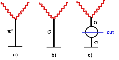
Figure 10: $\pi^{0}$ and $\sigma$ pole graphs.

Now we notice that Eq. (86) describes a computational method but not the $t$-channel Compton scattering process, which is described through

$$\gamma\gamma\to\sigma\to N\bar{N}.$$ (87)

The reason is that in the Compton scattering process only one intermediate state is possible, i.e. the creation of a $\sigma$ meson as part of the constituent-quark structure, whereas two or more intermediate states following each other are forbidden. This difference between computational method and $t$-channel Compton scattering is illustrated by the graphs in Figure 10. Graph b) describes the $t$-channel scattering process and graph c) the computational method where an intermediate pion loop is introduced so that the BEFT sum rule can be evaluated. On the basis of this consideration we can write down the scalar analog of Eq. (85) in the form

$$A^{{\sigma}+f_{0}+a_{0}}_{1}(t)=\frac{g_{{\sigma}NN}{\cal M}(\sigma\to\gamma\gamma)}{t-m^{2}_{\sigma}}+\frac{g_{{f_{0}}NN}{\cal M}(f_{0}\to\gamma\gamma)}{t-m^{2}_{f_{0}}}+\frac{g_{{a_{0}}NN}{\cal M}(a_{0}\to\gamma\gamma)}{t-m^{2}_{a_{0}}}\tau_{3}.$$ (88)

At this point the mass $m_{\sigma}$ is a parameter and it has to be clarified how the mass $m_{\sigma}$ has to be interpreted. This will be done in the next subsection.

5.4 Structure of the $\sigma$ meson

We restrict the present outline to the main argument and refer to [77, 78, 23] for further details. The $\sigma$ meson is a strongly decaying particle which may be described by a propagator in its most general form

$$P(s)=\frac{1}{m^{2}_{b}+\Pi(s)-s}$$ (89)

where $m_{b}$ is the “bare” mass and $\Pi(s)$ a “vacuum polarization function” [77, 78]. The imaginary part of $\Pi(s)$ may be obtained from unitarity considerations applied to the meson-meson decay channels. Since the “vacuum polarization function”, $\Pi(s)$, is analytic, its real part can be deduced from the imaginary part by making use of a dispersion relation. In a further step we may write the propagator in the form

$$P(s)=\frac{1}{m^{2}(s)-s-i\,m_{\rm BW}\Gamma_{\rm tot}(s)},$$ (90)

having identified

$$\Gamma_{\rm tot}=-\frac{{\rm Im}\Pi(s)}{m_{\rm BW}}$$ (91)

and

$$m^{2}(s)=m^{2}_{b}+{\rm Re}(s)$$ (92)

where $m^{2}(s)$ is the running mass square and $m_{\rm BW}$ the Breit-Wigner mass given by

$$m^{2}_{\rm BW}=m^{2}_{b}+{\rm Re}\Pi(m^{2}_{\rm BW}).$$ (93)

Up to this point the variable $s$ is a real quantity. But it is possible to shift this variable $s$ into the complex plane such that the denominator in Eq. (89) is equal to zero. Then the propagator may be written in the form

$$P(s)=\frac{1}{s_{R}-s}$$ (94)

corresponding to a pole on the second Riemann sheet at $s_{R}=(M_{R}-\frac{1}{2}\,i\,\Gamma_{R})^{2}$. For the $\sigma$-meson the “bare” mass² is $m_{\sigma}=666$ MeV (see [21] and the next subsection) whereas for the quantities $M_{\sigma}$ and $\Gamma_{\sigma}$ the results $M_{\sigma}=441^{+16}_{-8}$ MeV and $\Gamma_{\sigma}=544^{+18}_{-25}$ [79] have been obtained. Further details may be found in [21, 80].

In case of Compton scattering the two-photon fusion reaction $\gamma\gamma\to\sigma\to N\bar{N}$ has to be considered instead of the reaction $\gamma\gamma\to\sigma\to\pi\pi$. This leads to the consequence that $\Pi(s)\equiv 0$, because obviously there is no open meson-meson decay channel. Therefore, the propagator given in Eq. (89) has the form

$$P(s)=\frac{1}{m^{2}_{b}-s}.$$ (95)

For the Compton scattering amplitudes the pole described in Eq. (95) corresponds to a pole on the positive $t$-axis at $t_{0}=m^{2}_{b}$. This leads to the scalar pole terms given in Eq. (88) by identifying $m_{b}$ with $m_{\sigma}$ and the other masses, respectively.

5.5 The quark level linear $\sigma$ model (QLL$\sigma$M)

Now we come to the fundamental problem how the $\sigma$ meson and the other scalar mesons enter into the structure of the nucleon. First we notice that quite obviously the constituent quarks couple to all mesons having a nonzero meson-quark coupling constant. This statement is nontrivial because there are approaches where only Goldstone bosons are taken into consideration. Second we restrict the discussion to $SU(2)$ and refer to a generalization to $SU(3)$ given in [23]. Then we arrive at the description of chiral symmetry breaking given in the following.

The QLL$\sigma$M [29] combines the linear $\sigma$ model (96) with two versions of the Nambu–Jona-Lasinio model [81], the four-fermion versions of Eq. (97) and bosonized versions of Eq. (98)

$${\cal L}_{\sigma}=\frac{1}{2}\partial_{\mu}\mbox{\boldmath$\pi$}\cdot\partial^{\mu}\mbox{\boldmath$\pi$}+\frac{1}{2}\partial_{\mu}\sigma\partial^{\mu}\sigma+\frac{\mu^{2}}{2}(\sigma^{2}+\mbox{\boldmath$\pi$}^{2})-\frac{\lambda}{4}(\sigma^{2}+\mbox{\boldmath$\pi$}^{2})^{2}+f_{\pi}m^{2}_{\pi}\sigma,$$ (96)

$${\cal L}_{\rm NJL}=\bar{\psi}(i\mbox{$/\!\!\!\partial$}-m_{0})\psi+\frac{G}{2}[(\bar{\psi}\psi)^{2}+(\bar{\psi}i\gamma_{5}\mbox{\boldmath$\tau$}\psi)^{2}],$$ (97)

$${\cal L^{\prime}}_{\rm NJL}=\bar{\psi}i\mbox{$/\!\!\!\partial$}\psi-g\bar{\psi}(\sigma+i\gamma_{5}\mbox{\boldmath$\tau$}\cdot\mbox{\boldmath$\pi$})\psi-\frac{1}{2}\delta\mu^{2}(\sigma^{2}+\mbox{\boldmath$\pi$}^{2})+\frac{gm_{0}}{G}\sigma,$$ (98)

$$G=g^{2}/\delta\mu^{2},\quad\delta\mu^{2}=(m^{\rm cl}_{\sigma})^{2},\quad G=\lambda/(\sqrt{2}m^{\rm cl}_{\sigma})^{2},\quad g=\sqrt{\lambda/2},$$ (99)

where $m^{\rm cl}_{\sigma}$ denotes the mass of the $\sigma$ meson in the chiral limit (cl). Eq. (96) describes spontaneous chiral symmetry breaking in terms of fields where a mexican hat potential is introduced, parameterized by the mass parameter $\mu^{2}>0$ and the self-coupling parameter $\lambda>0$. Explicit symmetry breaking is taken into account by the last term which vanishes in the chiral limit $m_{\pi}\to 0$. In contrast to this Eqs. (97) and (98) describe dynamical chiral symmetry breaking in terms of $u$ and $d$ constituent quarks as the relevant fermions. In Eq. (97) the interaction between the fermions is parameterized by the four-fermion interaction constant $G$ and explicit symmetry breaking by the average current-quark mass $m_{0}$. Eq. (98) differs from (97) by the fact that the interaction is described by the exchange of bosons. This leads to the occurrence of a mass counter term parameterized by $\delta\mu^{2}$. Eq. (99) shows how these different parameters are related to each other.

In more detail, the bosonization starts with the following ansatz [82]

$$\sigma=-\frac{G}{g}\bar{\psi}\psi,$$ (100)

$$\mbox{\boldmath$\pi$}=-\frac{G}{g}\bar{\psi}\,i\,\gamma_{5}\mbox{\boldmath$\tau$}\,\psi.$$ (101)

This ansatz leads to the relation

$$-\frac{g^{2}}{2G}(\sigma^{2}+\mbox{\boldmath$\pi$}^{2})-\bar{\psi}\,g\,(\sigma+i\,\gamma_{5}\mbox{\boldmath$\tau$})\psi=\frac{G}{2}\left[(\bar{\psi}\psi)^{2}+(\bar{\psi}i\,\gamma_{5}\,\mbox{\boldmath$\tau$}\,\psi)^{2}\right]$$ (102)

and therefore converts

$${\cal L}=\bar{\psi}(i\,/\!\!\!\partial-m_{0})\psi+\frac{G}{2}\left[(\bar{\psi}\psi)^{2}+\bar{\psi}i\,\gamma_{5}\,\mbox{\boldmath$\tau$}\,\psi)^{2}\right]$$ (103)

into

$${\cal L}=\bar{\psi}(i\,/\!\!\!\partial-g(\sigma+\mbox{\boldmath$\pi$}\cdot\mbox{\boldmath$\tau$}\,\gamma_{5}))\psi-\frac{g^{2}}{2G}(\sigma^{2}+\mbox{\boldmath$\pi$}^{2})+\frac{gm_{0}}{G}\sigma.$$ (104)

The use of two versions of the NJL model has the advantage that for many applications the four-fermion version is more convenient whereas the bosonized version describes the interaction of the constituent quark with the QCD vacuum through the exchange of the $(\mbox{\boldmath$\pi$},\sigma)$ meson quartet which we consider as the true description of the physical process.

Using diagrammatic techniques the following equations may be found [83, 84] for the non-strange $(\mbox{\boldmath$\pi$},\sigma)$ sector

$$M^{*}=m_{0}+8\,i\,GN_{c}\int^{\Lambda}\frac{d^{4}p}{(2\pi)^{4}}\frac{M^{*}}{p^{2}-M^{*2}},\quad M=-\frac{8\,iN_{c}g^{2}}{(m^{\rm cl}_{\sigma})^{2}}\int\frac{d^{4}p}{(2\pi)^{4}}\frac{M}{p^{2}-M^{2}},$$ (105)

$$f^{2}_{\pi}=-4\,i\,N_{c}M^{*2}\int^{\Lambda}\frac{d^{4}p}{(2\pi)^{4}}\frac{1}{(p^{2}-M^{*2})^{2}},\quad f^{\rm cl}_{\pi}=-4iN_{c}gM\int\frac{d^{4}p}{(2\pi)^{4}}\frac{1}{(p^{2}-M^{2})^{2}}.$$ (106)

The expression given on the l.h.s. of (105) is the gap equation with $M^{*}$ being the mass of the constituent quark with the contribution $m_{0}$ of the current quarks included. The r.h.s. shows the gap equation for the nonstrange $(n\bar{n})$ constituent-quark mass $M$ in the chiral limit. The l.h.s. of Eq. (106) represents the pion decay constant and the r.h.s. the same quantity in the chiral limit. For further details we refer to [16, 29].

Making use of dimensional regularization the Delbourgo-Scadron [29] relation

$$M=\frac{2\pi}{\sqrt{N_{c}}}f^{\rm cl}_{\pi},\quad N_{c}=3$$ (107)

may be obtained from the r.h.s of Eqs. (105) and (106). This important relation shows that the mass of the constituent quark in the chiral limit and the pion decay constant in the chiral limit are proportional to each other. This relation is valid independent of the flavor content of the constituent quark, e.g. also for a constituent quark where the $d$-quark is replaced by a $s$-quark. Furthermore, it has been shown [85, 86] that (107) is valid independent of the regularization scheme.

An update for the mass prediction for the $\sigma$ mesons is obtained by using the more recent result for the pion decay constant as given in [39]. This leads to the neutral-pion decay constant

$$f_{\pi}=(92.21\pm 0.15)\,\,{\rm MeV}$$ (108)

and via a once-subtracted dispersion relation [87]

$$1-\frac{f^{\rm cl}_{\pi}}{f_{\pi}}=\frac{m^{2}_{\pi}}{8\pi^{2}f^{2}_{\pi}}=2.8\%$$ (109)

to

$$f^{\rm cl}_{\pi}=f_{\pi}(1-0.028)=89.63\,\,{\rm MeV}.$$ (110)

Then the update of the mass of the $\sigma$ meson is

$$m^{\rm cl}_{\sigma}=650.3\,\,{\rm MeV}$$ (111)

and

$$m_{\sigma}=[(m^{\rm cl}_{\sigma})^{2}+{\hat{m}}^{2}_{\pi}]^{1/2}=664\,\,{\rm MeV}$$ (112)

which agrees with the standard value [16] $m_{\sigma}=666$ MeV within 0.3%.

It is interesting to note that the QLL$\sigma$M for $N_{c}=3$ nonperturbatively predicts the parameters of the potential entering into the linear $\sigma$ model to be $\lambda=\frac{8\pi^{2}}{3}=26.3$ and $\mu=\sqrt{\frac{2}{3}}2\pi f^{\rm cl}_{\pi}=459.8$ MeV, whereas these quantities remain undetermined when only spontaneous symmetry breaking as given in (96) is considered.

For sake of completeness we wish to mention that in addition to the aspects of the QLL$\sigma$M as outlined above we may write the SU(2) interaction part of the QLL$\sigma$M Lagrangian density in the form [29, 30]

$${\cal L}_{L\sigma M}^{\rm int}=g\bar{\psi}(\sigma+i\gamma_{5}\mbox{\boldmath$\tau$}\cdot\mbox{\boldmath$\pi$})\psi+g^{\prime}\sigma(\sigma^{2}+\mbox{\boldmath$\pi$}^{2})-\frac{\lambda}{4}(\sigma^{2}+\mbox{\boldmath$\pi$}^{2})^{2}.$$ (113)

Here $\sigma$ denotes the $\sigma$ field after the shift of its origin to the vacuum expectation value $f_{\pi}$ has been carried out. The fermion fields refer to constituent quarks as described in [29, 30]. Eq. (113) allows to generate expression for the $\pi-\sigma-\pi$ and $\sigma-\sigma-\sigma$ coupling constants which, however, are not of importance for the present considerations.

Of the different options to describe chiral symmetry breaking we adopt the bosonized NJL model as the one which describes the $\sigma$ meson as part of constituent-quark structure in the most transparent way. The linear $\sigma$ model is only discussed for sake of completeness. Simultaneously a definite prediction of the $\sigma$ meson mass is obtained. The prediction of the transition amplitude ${\cal M}(\sigma\to\gamma\gamma)$ requires the knowledge of the quark-structure of the $\sigma$ meson where we have the option of a $q\bar{q}$ structure and a tetraquark structure. As has been shown in detail in [23] these two options do not make a difference in the present case because the two-photon interaction takes place with the $q\bar{q}$ structure in any case. This $q\bar{q}$ structure either serves as the intermediate state in nucleon Compton scattering or as a doorway state in case of the tetraquark structure [23] in the reaction chain $\gamma\gamma\to(u\bar{u}+d\bar{d})/\sqrt{2}\to u\bar{u}d\bar{d}\to\pi\pi$. Therefore, the $q\bar{q}$ structure may be used for the prediction of ${\cal M}(\sigma\to\gamma\gamma)$.

The results obtained in the present subsection may be compared with a more general treatment of the topic in “Constituent-quark masses and the electroweak standard model” [88].

5.6 The QLL$\sigma$M and polarizabilities

As before we start with pseudoscalar mesons and the corresponding spin-polarizability and thereafter turn to scalar mesons and the corresponding polarizability difference $(\alpha-\beta)^{t}$.

The main part of the $t$-channel component of the backward spinpolarizability is given by

$$|\pi^{0}\rangle=\frac{1}{\sqrt{2}}(-|u\bar{u}\rangle+|d\bar{d}\rangle),\quad{\cal M}(\pi^{0}\to\gamma\gamma)=\frac{\alpha_{em}N_{c}}{\pi f_{\pi}}\left[-\left(\frac{2}{3}\right)^{2}+\left(\frac{-1}{3}\right)^{2}\right],$$ (114)

$${\gamma_{\pi}^{t}}_{(p,n)}=\frac{g_{\pi^{0}NN}\quad{\cal M}(\pi^{0}\to\gamma\gamma)}{2\pi m^{2}_{\pi^{0}}m}\tau_{3}=-46.7\,\tau_{3}\,\,\,{10}^{-4}{\rm fm}^{4}.$$ (115)

Analogously, we obtain for the main $t$-channel parts of the electric ($\alpha$) and magnetic ($\beta$) polarizabilities the relations

$$|\sigma\rangle=\frac{1}{\sqrt{2}}(|u\bar{u}\rangle+|d\bar{d}\rangle),\quad{\cal M}(\sigma\to\gamma\gamma)=\frac{\alpha_{em}N_{c}}{\pi f_{\pi}}\left[\left(\frac{2}{3}\right)^{2}+\left(\frac{-1}{3}\right)^{2}\right],$$ (116)

$$(\alpha-\beta)^{t}_{p,n}=\frac{g_{\sigma NN}{\cal M}(\sigma\to\gamma\gamma)}{2\pi m^{2}_{\sigma}}=15.2\,\,\,{10}^{-4}{\rm fm}^{3},\quad(\alpha+\beta)^{t}_{p,n}=0,$$ (117)

$$\alpha^{t}_{p,n}=+7.6\,\,\,{10}^{-4}{\rm fm}^{3},\,\beta^{t}_{p,n}=-7.6\,\,{10}^{-4}{\rm fm}^{3},$$ (118)

where use is made of $g_{\pi NN}=g_{\sigma NN}=13.169\pm 0.057$ [89] and $m_{\sigma}=664$ MeV as predicted by the QLL$\sigma$M. The sign convention used in the $q\bar{q}$ structure of the $\pi^{0}$ meson follows from [90]. It has the advantage of correctly predicting the sign of the $\pi^{0}$-pole contribution. These main contributions to the polarizabilities $\alpha$, $\beta$ and $\gamma_{\pi}$ have to be supplemented by the $s$-channel components and by the small components due to the scalar mesons $f_{0}(980)$ and $a_{0}(980)$ in case of the polarizabilities $\alpha$ and $\beta$ and due to the pseudoscalar meson $\eta$ and $\eta^{\prime}$ in case of $\gamma_{\pi}$.

The appropriate tool for the prediction of the polarizabilities $\alpha$ and $\beta$ is to simultaneously apply the forward-angle sum rule for $(\alpha+\beta)$ and the backward-angle sum rule for $(\alpha-\beta)$. This leads to the relations derived in [17, 20] and shown in subsection 2.5. From the expression for the scalar $t$-channel amplitude given in (88) we obtain

$$(\alpha-\beta)^{t}=\frac{g_{\sigma NN}{\cal M}(\sigma\to\gamma\gamma)}{2\pi m^{2}_{\sigma}}+\frac{g_{f_{0}NN}{\cal M}(f_{0}\to\gamma\gamma)}{2\pi m^{2}_{f_{0}}}+\frac{g_{a_{0}NN}{\cal M}(a_{0}\to\gamma\gamma)}{2\pi m^{2}_{a_{0}}}\tau_{3},$$ (119)

and with $(\alpha+\beta)^{t}=0$

$$\alpha^{t}=\frac{1}{2}(\alpha-\beta)^{t},$$ (120)

$$\beta^{t}=-\frac{1}{2}(\alpha-\beta)^{t}.$$ (121)

.

The $t$-channel part of the backward spin-polarizability is given by [18, 38]

$$\gamma^{t}_{\pi}=\frac{1}{2\pi m}\left[\frac{g_{\pi NN}{\cal M}(\pi^{0}\to\gamma\gamma)}{m^{2}_{\pi^{0}}}\tau_{3}+\frac{g_{\eta NN}{\cal M}(\eta\to\gamma\gamma)}{m^{2}_{\eta}}+\frac{g_{\eta^{\prime}NN}{\cal M}(\eta^{\prime}\to\gamma\gamma)}{m^{2}_{\eta^{\prime}}}\right].$$ (122)

The numerical evaluation of these contributions has been described in detail in previous papers [18, 20]. Here we give a summary of the final predictions and the experimental values to compare with in Table 4 and 5.

Table 4: Backward spinpolarizabilities for the proton and the neutron [22] and Table 2

spin polarizabilities	$\gamma^{(p)}_{\pi}$	$\gamma^{(n)}_{\pi}$
$\pi^{0}$ pole	-46.7	+46.7
$\eta$ pole	+1.2	+1.2
$\eta^{\prime}$ pole	+0.4	+0.4
const. quark structure	$-$45.1	+48.3
nucleon structure	+8.5	+10.0
total predicted	$-$36.6	+58.3
exp. result	$-$($36.4\pm 1.5$)	+($58.6\pm 4.0$)
	unit 10-4 fm4

Table 5: Polarizabilities for the proton and the neutron [20] and Table 2

	$\alpha_{p}$	$\beta_{p}$	$\alpha_{n}$	$\beta_{n}$
$\sigma$ pole	+7.6	$-7.6$	+7.6	$-7.6$
$f_{0}$ pole	+0.3	$-0.3$	+0.3	$-0.3$
$a_{0}$ pole	$-0.4$	+0.4	+0.4	$-0.4$
const. quark structure	+7.5	$-7.5$	+8.3	$-8.3$
nucleon structure	+4.5	+9.4	+5.1	+10.1
total predicted	+12.0	+1.9	+13.4	+1.8
exp. result	+($12.0\pm 0.6$)	+($1.9\mp 0.6$)	+($12.5\pm 1.7$)	+($2.7\mp 1.8$)
	unit 10-4 fm3

The most interesting feature of the polarizabilities as given in Table 5 is the strong cancellation of the paramagnetic polarizabilities which is mainly due to the $P_{33}(1232)$ resonance by the diamagnetic term which is solely due to the constituent-quark structure.

A further interesting conclusion concerns the two-photon width of the $\sigma$ mesons which can be calculated from the data given in (116). Given the nonperturbative QLL$\sigma$M $\sigma$ meson mass of 664 MeV the amplitude for the $\sigma\to\gamma\gamma$ decay for $N_{c}=3$ and $f_{\pi}=92.21$ MeV is

$${\cal M}(\sigma\to\gamma\gamma)=\frac{5\,\alpha_{\rm em}}{3\pi f_{\pi}}=0.042\,\,\text{GeV}^{-1}$$ (123)

and the decay width

$$\Gamma_{\gamma\gamma}=\frac{m^{3}_{\sigma}}{64\pi}|{\cal M}(\sigma\to\gamma\gamma)|^{2}=2.6\,\,\text{keV}.$$ (124)

From Table 5 we obtain that the predicted and the experimental electric polarizabilities $\alpha_{p}$ of the proton are in excellent agreement with each other. Furthermore, the experimental quantity $\alpha_{p}$ has an experimental error of $\pm 5\%$ which may be used to calculated the experimental error of the two-photon width $\Gamma_{\gamma\gamma}$ of the $\sigma$ mesons. This rather straightforward consideration leads to $\Gamma_{\gamma\gamma}=2.6\pm 0.3$ keV [21].

6 Compton scattering in a large angular range and at energies up to 1 GeV

In the foregoing we have restricted our considerations to the forward and the backward directions. This is of advantage as long as we are interested in theoretical aspects of nucleon Compton scattering and polarizabilities, because transparent definitions of the polarizabilities are possible which may be used for theoretical predictions. Compton scattering experiments are only possible in an interval of intermediate angles ranging from about $\theta_{\rm lab}=30^{\circ}$ to $150^{\circ}$. This means that the experimental determination of polarizabilities can only be obtained from data measured at these intermediate angles. In addition to this the invariant amplitudes $A_{i}(s,t,u)$ (i=1–6) may be considered as generalized polarizabilities containing valuable information about interference effects between different phenomena contributing to the Compton scattering process. Of these the interference of scattering from the $s$-channel and the $t$-channel is of particular interest because it is related to degrees of freedom stemming from the photoexcitation of the nucleon on the one hand and from photoexcitation of the mesonic structure of the constituent quarks on the other.

Compton scattering by the nucleon at energies up to 1.2 GeV has been studied by many groups in different laboratories over a long period of time. The final interpretation of these experiments has been carried out by L’vov et al. in 1997 [34] where a precise method for the calculation of scattering amplitudes is developed, based on non-subtracted fixed-$t$ dispersion theory. This dispersion theory requires the introduction of asymptotic or $t$-channel contributions, leading to the introduction of the $\sigma$-meson pole amplitude in addition to the well known $\pi^{0}$-meson pole amplitude. At this status of development the large-angle Compton scattering experiment was carried at MAMI (Mainz) [32, 33] which is already described in the introduction. This experiment precisely confirmed the dispersion theory developed by L’vov et al. [34].

In spite of this great success fixed-$t$ dispersion theory has a disadvantage, because the integration paths for the $s$-channel dispersion relations are to a large extent in the unphysical region. This is not of relevance for the prediction of Compton differential cross sections but it makes the interpretation of the amplitudes intransparent.

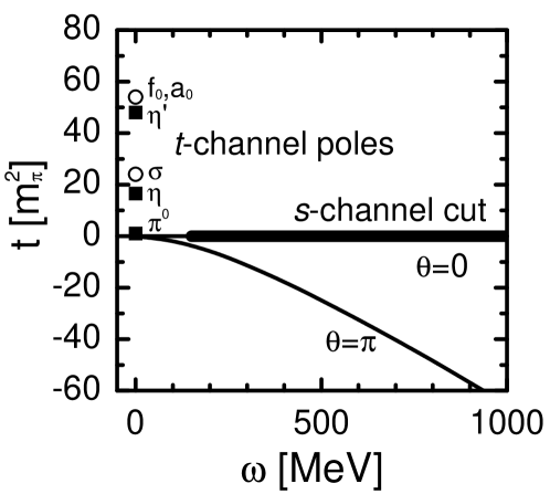
Figure 11: Singularities of the $s$- and the $t$-channel. Horizontal thick line: $s$-channel cut representing the nucleon (s-channel) degrees of freedom, with $\omega$ being the energy of the incoming photon in the lab system. Squares and circles on the vertical real $t$-axis: $t$-channel poles representing the constituent-quark degrees of freedom. The physical range of nucleon Compton scattering extends from the line at $\theta=0$ to the line at $\theta=\pi$.

For illustration Figure 11 shows the physical range of Compton scattering and the location of the singularities of the Compton scattering amplitudes in the $s$-$t$-plane. At $\theta=0$ the integration path of the dispersion integral coincides with the $s$-channel cut shown in Figure 11 which of course is located in the physical range. However, for larger negative $t$ the integration paths enter the area in the left part of the $s$-$t$-plan which is located outside the physical plane.

Subtracted fixed-$t$ dispersion theory [7, 56] has been applied and tested in the $\Delta$-resonance region and below but there is no information how it performs at higher energies. In order to overcome the disadvantages inherent in fixed-$t$ dispersion theories Drechsel et al. [7] have proposed to use hyperbolic dispersion relations which are essentially equivalent to fixed-$\theta$ dispersion relations. As will be outlined in the following the integration paths of hyperbolic dispersion relations keep the angle $\theta_{lab}$ fixed whereas the angle $\theta_{\rm cm}$ becomes dependent on the photon energy $\omega$. Fixed-$\theta$ or hyperbolic dispersion relations are easy to apply at $\theta=180^{\circ}$ but become increasingly uncertain at smaller angles. Especially, the evaluation of the $t$-channel contribution based on a scalar-isoscalar $t$-channel cut breaks down at scattering angles of $\theta_{\rm lab}<101^{\circ}$.

This difficulty may be avoided by replacing the $t$-channel cut by $t$-channel poles as provided by the QLL$\sigma$M. Since this new type of approach has never before been investigated it is appropriate to include a detailed description in the present status report.

6.1 Kinematics of Compton scattering

The conservation of energy and momentum in nucleon Compton scattering

$$\gamma(k,\lambda)+N(p)\to\gamma^{\prime}(k^{\prime},\lambda^{\prime})+N^{\prime}(p^{\prime})$$ (125)

is given by

$$k+p=k^{\prime}+p^{\prime}$$ (126)

where $k$ and $k^{\prime}$ are the 4-momenta of the incoming and outgoing photon and $p$ and $p^{\prime}$ the 4-momenta of incoming and outgoing proton. Mandelstam variables are introduced via

$$s=(k+p)^{2}=(k^{\prime}+p^{\prime})^{2},t=(k-k^{\prime})^{2}=(p^{\prime}-p)^{2},u=(k-p^{\prime})^{2}=(k^{\prime}-p)^{2},$$ (127)

$$s+t+u=2m^{2}.$$ (128)

with $m$ being the nucleon mass.

In terms of the Mandelstam variables the scattering angle $\theta$ in the cm system is given by

$$\sin^{2}\frac{\theta_{\rm cm}}{2}=-\frac{st}{(s-m^{2})^{2}}.$$ (129)

The $t$-channel corresponds to the fusion of two photons with four-momenta $k_{1}$ and $k_{2}$ and helicities $\lambda_{1}$ and $\lambda_{2}$ to form a $t$-channel intermediate state $|t\rangle$ from which – in a second step – a proton-antiproton pair is created. The corresponding reaction may be formulated in the form

$$\gamma(k_{1},\lambda_{1})+\gamma(k_{2},\lambda_{2})\to\bar{N}(p_{1})+N(p_{2}).$$ (130)

Since for Compton scattering the related $N\bar{N}$ pair creation-process is virtual, in dispersion theory we have to treat the process described in (130) in the unphysical region. In the cm frame of (130) where

$${\bf k_{1}}+{\bf k_{2}}=0$$ (131)

we obtain

$$\sqrt{t}=\sqrt{(k_{1}+k_{2})^{2}}=\omega_{1}+\omega_{2}=W^{t},$$ (132)

where $W^{t}$ is the energy transferred to the $t$-channel via two-photon fusion. At positive $t$ the $t$-channel of Compton scattering $\gamma N\to N\gamma$ coincides with the $s$-channel of the two-photon fusion reaction $\gamma_{1}+\gamma_{2}\to N\bar{N}$.

6.2 Hyperbolic dispersion relations

Hyperbolic dispersion relations have been introduced by Hite and Steiner [91] and further evaluated by Höhler [92] and Drechsel et al. [7]. Hyperbolic dispersion relations start with the ansatz

$$(s-a)(u-a)=(a-m^{2})^{2},\quad s+t+u=2m^{2},$$ (133)

where a new parameter $a$ is introduced. From (133) this new parameter is derived in the form

$$a=\frac{(s-m^{2})^{2}+st}{t},$$ (134)

or in terms of the cm scattering angle $\theta_{\rm cm}$ as given in (129) and the lab scattering angle $\theta_{\rm lab}$:

$$a=-s\frac{1-\sin^{2}\frac{1}{2}\theta_{\rm cm}}{\sin^{2}\frac{1}{2}\theta_{\rm cm}},\quad a=-m^{2}\frac{1-\sin^{2}\frac{1}{2}\theta_{\rm lab}}{\sin^{2}\frac{1}{2}\theta_{\rm lab}}.$$ (135)

After introducing the parameter $a$ hyperbolic dispersion relations may be written down in the form

$${\rm Re}A_{i}(s,t,a)=A^{B}_{i}(s,t,a)+A^{t-pole}_{i}(s,t,a)$$

$$\quad\quad\quad\quad\quad\,\,\,\,+\frac{1}{\pi}{\cal P}\int^{\infty}_{(m+m_{\pi})^{2}}\,ds^{\prime}\,{\rm Im}_{s}A_{i}(s^{\prime},{\tilde{t}},a)\left[\frac{1}{s^{\prime}-s}+\frac{1}{s^{\prime}-u}-\frac{1}{s^{\prime}-a}\right]$$

$$\quad\quad\quad\quad\quad\,\,\,\,+\frac{1}{\pi}{\cal P}\int^{\infty}_{0}\,dt^{\prime}\,\frac{{\rm Im}_{t}A_{i}({\tilde{s}},t^{\prime},a)}{t^{\prime}-t}$$ (136)

where $A^{B}_{i}(s,t,a)$ is the Born term and $A^{t-pole}_{i}(s,t,a)$ the pole in the $t$-channel. The discontinuity in the $s$-channel, ${\rm Im}_{s}(s^{\prime},{\tilde{t}},a)$, is evaluated along the path given by

$$(s^{\prime}-a)(u^{\prime}-a)=(a-m^{2})^{2},\quad s^{\prime}+{\tilde{t}}+u^{\prime}=2m^{2},$$ (137)

and the corresponding quantity of the $t$-channel, ${\rm Im}_{t}\,A_{i}({\tilde{s}},t^{\prime},a)$, along the path given by

$$({\tilde{s}}-a)({\tilde{u}}-a)=(a-m^{2})^{2},\quad{\tilde{s}}+t^{\prime}+{\tilde{u}}=2m^{2}.$$ (138)

The Mandelstam variables denoted by a tilde are those which do not enter directly into the dispersions integral, i.e. ${\tilde{t}}$ in case of the $s$-channel dispersion relation, and ${\tilde{s}}$ and ${\tilde{u}}$ in case of the $t$-channel dispersion relation.

6.3 Dispersion relations for the $s$-channel

Hyperbolic dispersion relations for the $s$-channel are given by the second line of Eq. (136). The last term in the square bracket is constructed such that it provides integration paths located in the physical range for all scattering angles. This is illustrated in Figure 12 where integration paths are given in a ${\tilde{t}}-\omega^{\prime}$ plane with

$$s^{\prime}=m^{2}+2m\,\omega^{\prime},$$ (139)

relating the Mandelstam variable $s^{\prime}$ to the photon energy $\omega^{\prime}$ in lab frame. The integration path (1) corresponds to $a=0$ and $\theta_{\rm lab}=180^{\circ}$, (2) red or black curve to $a=-m^{2}$ and $\theta_{\rm lab}=90^{\circ}$, (3) red or black curve to $a=-3\,m^{3}$ and $\theta_{\rm lab}=60^{\circ}$, (4) red or black curve to $a=-10\,m^{2}$ and $\theta_{\rm lab}=35.1^{\circ}$, (5) red or black curve to $a=-100\,m^{2}$ and $\theta_{\rm lab}=11.4^{\circ}$. Hyperbolic dispersion relations correspond to integration paths with constant $\theta_{\rm lab}$. In principle this is equivalent to using fixed-$\theta_{\rm cm}$ dispersion relations, except for the fact that slightly different integration paths have to be applied in order to cover the physical range of the ${\tilde{t}}-\omega^{\prime}$-plane. This is shown in Figure 12 where also fixed-$\theta_{cm}$ integration paths are given, represented by the green or grey curves. The only difference between these two options is that for the hyperbolic dispersion relations the $s$-channel parts have a somewhat more convenient form whereas the $t$-channel parts are identical in the two cases.

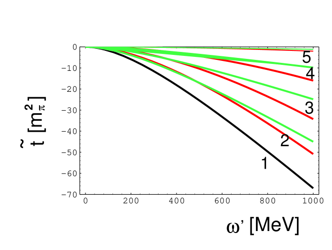
Figure 12: Integration paths of hyperbolic dispersion relations for different quantities $a$: (1) $a=0$ ($\theta_{\rm cm}\equiv\theta_{\rm lab}=180^{\circ}$), (2) red or black curve: $a=-m^{2}$ ($\theta_{\rm lab}=90^{\circ}$), green or grey curve: $\theta_{\rm cm}=110^{\circ}$ , (3) red or black curve: $a=-3\,m^{2}$ ($\theta_{\rm lab}=60^{\circ}$), green or grey curve: $\theta_{\rm cm}=75^{\circ}$ (4) red or black curve: $a=-10\,m^{2}$ ($\theta_{\rm lab}=35.1^{\circ}$), green or grey curve: $\theta_{\rm cm}=45^{\circ}$ , (5) red or black curve: $a=-100\,m^{2}$ ($\theta_{\rm lab}=11.4^{\circ}$), green or grey curve: $\theta_{\rm cm}=15^{\circ}$. In the forward direction ($\theta_{\rm cm}\equiv\theta_{\rm lab}=0^{\circ}$) we have $a\to\infty$.

It is interesting to note that the total backward hemisphere in the lab frame corresponds to the small range between integration path (1) and (2), whereas the forward hemisphere is spread out over a larger range in the physical ${\tilde{t}}-\omega^{\prime}$ plane. The important conclusion we may draw from this observation is that qualitative properties of the scattering amplitudes found at $\theta=180^{\circ}$ are also valid at smaller angles inside the backward hemisphere. This means that interference effects found at $\theta=180^{\circ}$ are also representative for smaller angles.

6.4 Dispersion relations for the $t$-channel

The $t$-channel singularities enter into the scattering amplitudes via $t$-poles as given in the first line of Eq. (136). These $t$-poles have an explicit $a$ or $\theta$ dependence except for $\theta=180^{\circ}$ where the Eqs. (85) and(88) are valid. Since explicit expressions for the $\theta$ dependence of the $t$-poles have not been derived up to now this will be done in the following.

As an introduction we consider the well-known case of $\theta=180^{\circ}$ and then generalize the results by including smaller scattering angles. At $\theta=180^{\circ}$ the kinematical constraints are

$$s¸\,u=m^{4},\quad\quad s+t+u=2\,m^{2},$$ (140)

being equivalent with

$$t=-\frac{(s-m^{2})^{2}}{s}.$$ (141)

Using (141) we have to find the topological manyfold in the complex $s$-plane where $t$ is a non-negative real number. This problem has been solved in [27, 28] where it has been shown that this topological manyfold is given by

$$s=m^{2}\,e^{i\,\alpha}$$ (142)

leading to

$$t=4m^{2}\sin^{2}\frac{\alpha}{2}.$$ (143)

This consideration shows that even in the case of $\theta=180^{\circ}$ where the poles of Eqs. (85) and (88) are independent of $s$ the two variables $s$ and $t$ constrain each other.

It is important to note that the convenient representation (142) of the topological manifold is the only result borrowed from [27, 28]. Especially we use different dispersion relations and do not make explicit use of the circle (142) in the complex $s$-plane. For the following only Eq. (143) is of importance which contains the constraints of the variable $t$ in a transparent way.

After this introductory remark it is easy to find the corresponding constraints for the case of $\theta<180^{\circ}$. First we notice that the condition

$$(s-a)(u-a)=(a-m^{2})^{2}\quad\quad s+t+u+=2m^{2}$$ (144)

is equivalent with

$$x=\frac{t}{\sin^{2}\frac{\theta_{\rm cm}}{2}}=-\frac{(s-m^{2})^{2}}{s}=4m^{2}\sin^{2}\frac{\alpha}{2}.$$ (145)

This means that for $\theta<180^{\circ}$ we have exactly the same kinematical relation as in case of $\theta=180^{\circ}$, except for the fact that the variable $t$ is replaced by the variable

$$x=\frac{t}{\sin^{2}\frac{\theta_{\rm cm}}{2}}.$$ (146)

The $t$-channel part of the dispersion relation in (136) may now be written in terms of the parameter $x$ instead of the parameter $t$. The advantage of this parameter transformation is that it takes care of the kinematical constraints of Eq. (144). Since $t$ is a nonnegative real number (145) implies a constraint in the form

$$0\leq\sin^{2}\left(\frac{\alpha}{2}\right)\leq 1,\quad 0\leq t\leq t_{max}=4\,m^{2}\sin^{2}\left(\frac{\theta_{\rm cm}}{2}\right).$$ (147)

Then with

$$x=4\,m^{2}\sin^{2}\left(\frac{\alpha}{2}\right),\quad x_{0}=\frac{\mu^{2}}{\sin^{2}\left(\frac{\theta_{\rm cm}}{2}\right)}$$ (148)

we arrive at

$$A^{t-pole}_{i}(t,\theta)={\cal M}(M\to\gamma\gamma)\,g_{MNN}\int^{4\,m^{2}}_{0}\frac{\delta(x-x_{0})}{x^{\prime}-x}dx^{\prime}=\frac{{\cal M}(M\to\gamma\gamma)g_{MNN}}{t-\mu^{2}}\sin^{2}\left(\frac{\theta_{\rm cm}}{2}\right)$$ (149)

$$(i=1,2)$$

for a meson $M$ with mass $\mu$. The amplitude given in (6.4) is the solution of the $t$-channel integral of Eq.(136).

Eq. (147) implies that there exists a further constraint related to the mass of the meson, given by

$$\mu^{2}\leq 4\,m^{2}\sin^{2}\left(\frac{\theta_{\rm cm}}{2}\right).$$ (150)

Because of this relation, the finite masses of the mesons imply that the amplitudes $A_{i}(t,\theta)$ (i=1,2) vanish below a lower limit $\theta_{\rm lim}$ of the cm scattering angle. These lower limits are $\theta_{\rm lim}(\pi^{0})=8.2^{\circ}$, $\theta_{\rm lim}(\eta)=34.0^{\circ}$, $\theta_{\rm lim}(\sigma)=41.6^{\circ}$, $\theta_{\rm lim}(\eta^{\prime})=61.3^{\circ}$ and $\theta_{\rm lim}(f_{0},a_{0})=62.9^{\circ}$.

6.5 Interference between nucleon and constituent-quark structure Compton scattering

Hyperbolic dispersion relations as outlined above may be applied to a calculation of Compton differential cross sections in the whole angular range and for photon energies up to 1 GeV where precise photo-absorption cross sections are available. In this way the successful calculations [34, 32, 33] in terms of fixed-$t$ dispersions relations could be reproduced by an independent computational procedure.

The most interesting application of course is the study of interference phenomena of constituent-quark structure ($t$-channel) and nucleon-structure ($s$-channel) Compton scattering amplitudes. This will be carried out in the following by investigating the energy dependence of the polarizabilities $(\alpha-\beta)$ and $\gamma_{\pi}$.

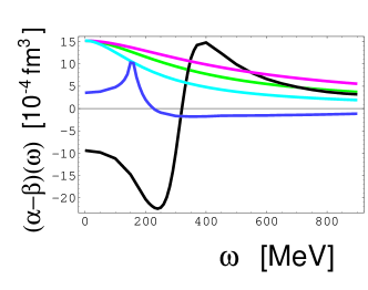
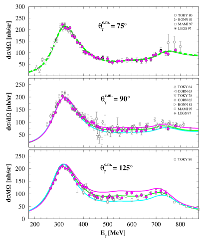
Figure 13: Left panel: Difference of generalized polarizabilities $(\alpha-\beta)(\omega)$ versus photon energy $\omega$. Solid curve starting at $(\alpha-\beta)(0)=-9.4$: contribution of the $P_{33}(1232)$ resonance. Solid curve starting at $(\alpha-\beta)(0)=+3.5$: Contribution of the nonresonant $E_{0+}$ amplitude. Curves starting at $(\alpha-\beta)(0)=+15.2$: $t$-channel contribution of the $\sigma$ meson calculated for different $\sigma$-meson masses. Upper curve (dark grey or red): $m_{\sigma}=800$ MeV. Middle curve (grey or green): $m_{\sigma}=600$ MeV. Lower curve (light grey or blue): $m_{\sigma}=400$ MeV. Not shown is the contribution of the $D_{13}(1520)$ resonance which cancels the $E_{0+}$ contribution in the relevant energy range from 400 to 700 MeV. Right panel: Differential cross sections for Compton scattering by the proton versus photon energy. The three panels contain data corresponding to the cm-angles of $75^{\circ}$, $90^{\circ}$ and $125^{\circ}$. The three curves are calculated for different mass parameters $m_{\sigma}=800$ MeV (upper, dark grey or red), 600 MeV (center, grey or green) and 400 MeV (lower, light grey or blue).

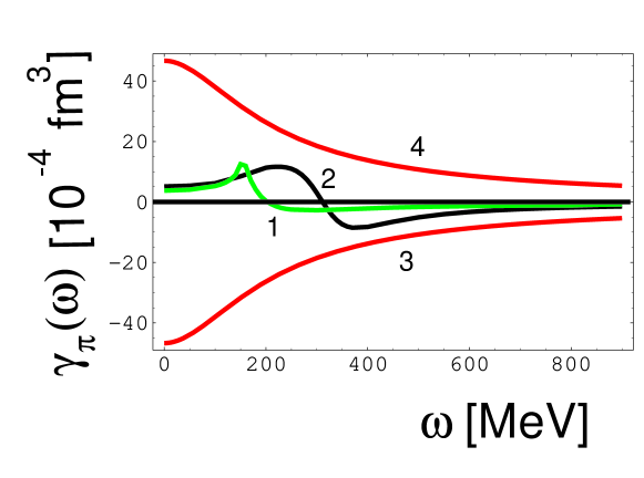
Figure 14: Energy dependent backward spinpolarizability $\gamma_{\pi}(\omega)$ versus photon energy $\omega$ in the lab frame. Curve 1: Contribution due to the $E_{0+}$ CGLN amplitude, curve 2: Contribution due to the $P_{33}(1232)$ resonance, curve 3: $t$-channel contribution for the proton, curve 4: $t$-channel contribution for the neutron.

For this purpose we introduce linear combinations of invariant amplitudes which contain these energy dependent polarizabilities [1]:

$${\tilde{A}}_{1}(s,u,t)\equiv A_{1}(s,u,t)-\frac{t}{4m^{2}}A_{5}(s,u,t),$$ (151)

$${\tilde{A}}_{2}(s,u,t)\equiv A_{2}(s,u,t)+\left(1-\frac{t}{4m^{2}}\right)A_{5}(s,u,t).$$ (152)

Then the $\omega$-dependent “dynamical” polarizabilities are given by

$$(\alpha-\beta)(\omega)=(\alpha-\beta)^{s}(\omega)+(\alpha-\beta)^{t}(\omega)=-\frac{1}{2\pi}{\rm Re}{\tilde{A}}^{\rm nB}_{1}(s,t,a=0),$$ (153)

$$\gamma_{\pi}(\omega)=\gamma^{s}_{\pi}(\omega)+\gamma^{t}_{\pi}(\omega)=-\frac{1}{2\pi\,m}{\rm Re}{\tilde{A}}^{\rm nB}_{2}(s,t,a=0).$$ (154)

In (153) and (154) nB denotes that non-Born parts of the respective amplitudes have to be taken into account. The $\omega$-dependent “dynamical” polarizabilities are constructed such that they coincide with the conventional $\omega$-independent polarizabilities in the limits $s=m^{2}$, $u=m^{2}$, and $t=0$.

The application of hyperbolic dispersion relations for $\theta=\pi$ leads to

$$(\alpha-\beta)^{s}(\omega)=\frac{1}{2\pi^{2}}{\cal P}\int^{\infty}_{\omega_{0}}\sqrt{1+2\frac{\omega^{\prime}}{m}}F(\omega^{\prime},\omega)(\sigma(\omega^{\prime},\Delta P={\rm yes})-\sigma(\omega^{\prime},\Delta P={\rm no}))\frac{d\omega^{\prime}}{\omega^{\prime 2}},$$

$$(\alpha-\beta)^{t}=-\frac{1}{2\pi}\frac{{\cal M}(\sigma\to\gamma\gamma)g_{\sigma NN}}{t(\omega)-m^{2}_{\sigma}},$$ (155)

$$\gamma^{s}_{\pi}(\omega)=\frac{1}{4\pi^{2}}{\cal P}\int^{\infty}_{\omega_{0}}\sqrt{1+2\frac{\omega^{\prime}}{m}}\left(1+\frac{\omega^{\prime}}{m}\right)F(\omega^{\prime},\omega)\Sigma_{n}P_{n}\left(\sigma^{n}_{3/2}(\omega^{\prime})-\sigma^{n}_{1/2}(\omega^{\prime})\right)\frac{d\omega^{\prime}}{\omega^{\prime 3}},$$

$$\gamma^{t}_{\pi}=-\frac{1}{2\pi\,m}\frac{{\cal M}(\pi^{0}\to\gamma\gamma)g_{\pi NN}}{t(\omega)-m^{2}_{\pi^{0}}}\tau_{3},$$ (156)

with

$$F(\omega^{\prime},\omega)=\frac{\omega^{\prime 3}+\omega^{\prime 2}(m/2)}{\omega^{\prime 3}+\omega^{\prime 2}a(\omega)+\omega^{\prime}b(\omega)+c(\omega)},\quad\omega_{0}=m_{\pi}+\frac{m^{2}_{\pi}}{2m},$$ (157)

$$a(\omega)=\frac{-4\omega^{2}+2m\omega+m^{2}}{2(m+2\omega)},\quad\quad\,\,b(\omega)=-\frac{2m\omega^{2}}{m+2\omega},$$ (158)

$$c(\omega)=-\frac{m^{2}\omega^{2}}{2(m+2\omega)},\quad\quad\quad\quad\quad\quad t(\omega)=-4\frac{\omega^{2}}{1+2\frac{\omega}{m}}.$$ (159)

The quantity $\Delta P$ denotes parity change (yes) or nonchange (no), the parity factor is $P_{n}=-1$ for $\Delta P=$ yes and $P_{n}=+1$ for $\Delta P=$ no. The function $F(\omega^{\prime},\omega)$ contains the $\omega$ dependence of the $s$-channel parts of the polarizabilities and converges like $F(\omega^{\prime},\omega)\to 1$ for $\omega\to 0$.

The results obtained from the evaluation of Eq. (155) are shown in the left panel of Figure 13. It is clearly demonstrated that there is a constructive interference in the energy range from 400 to 700 MeV between the contribution from the $P_{33}(1232)$ resonance and from the $t$-channel due to the $\sigma$ meson as part of the constituent-quark structure. The sum of the two contributions depends on the mass of the $\sigma$ meson assumed in the calculation and, therefore, may be used for a determination of the $\sigma$-meson mass $m_{\sigma}$ from the differential cross section for Compton scattering. This is outlined in the right panel of Figure 13 where the effects of the $\sigma$-meson mass are most prominent in the backward direction, as expected. The best agreement is obtained for $m_{\sigma}=600$ MeV, being compatible with our present knowledge of the “bare” mass¹ of the $\sigma$ meson. As pointed out before [21] the experimental data shown in Figure 13 may be interpreted as a direct observation of the $\sigma$ meson while being part of the constituent-quark structure. Furthermore, this experiment provides us with the first and only direct determination of the “bare” mass¹ of the $\sigma$ meson, whereas in all the other observations of the $\sigma$ meson the Breit-Wigner parameters or the position of the pole on the second Riemann sheet are determined.

Eq.(154) provides a possibility to study interference effects of the $t$-channel $\pi^{0}$ contribution with the contribution from the $P_{33}(1232)$. Because of the smaller mass of the $\pi^{0}$ meson as compared with the $\sigma$ meson the relevant energy range is at lower energies. The interference pattern is shown in Figure 14. The largest interference effect is seen in the energy range between 200 and 300 MeV. In this range the interference is destructive in case of the proton and constructive in case of the neutron.

In Figures 13 and 14 we have shown that there are pronounced interference terms from the $t$-channel constributions and the contributions from the $P_{33}(1232)$ resonance for $(\alpha-\beta)(\omega)$ as well as for $\gamma_{\pi}(\omega)$. These interference terms in the two cases allow to determine an error for the mass $m_{\sigma}$ of the $\sigma$ meson due to uncertainties of the CGLN amplitude representing the $P_{33}(1232)$ resonance. The evaluation of $\gamma_{\pi}^{(p)}$ and $m_{\sigma}$ from the data of the LARA experiment [32, 33] were based on the SAID-SM99K parameterization, with the MAID2000 parameterization used for comparison. The results given in Table 6 were obtained (see also [1]):

Table 6: Evaluation of $\gamma^{(p)}_{\pi}$ and $m_{\sigma}$ using data from the LARA experiment [32, 33]

	SAID-SM99K	MAID2000
$\gamma^{(p)}_{\pi}$	$-37.1$	$-40.9$	LARA experiment [32, 33]
$m_{\sigma}$	600 MeV	400 MeV	LARA experiment [32, 33]

where LARA denotes the experiment leading to the results shown in Figure 13. For $\gamma^{(p)}_{\pi}$ the SAID-SM99K parameterization leads to agreement with the present recommended value $\gamma^{(p)}_{\pi}=-36.4\pm 1.5$ (experiment), -36.6 (predicted) whereas MAID2000 leads to results shifted by 10%. By the same procedure $m_{\sigma}$ is shifted by $\Delta m_{\sigma}=-200$ MeV. Since the present recommended values are based on the most recent and very precise CGLN amplitudes [24] we can say that the evaluations of $\gamma^{(p)}_{\pi}$ and $m_{\sigma}$ on the bases of the SAID-SM99K parameterization have been confirmed on a high level of precision, whereas the use of the MAID2000 parameterization has been ruled out. Nevertheless, the shifts of the results for $\gamma^{(p)}_{\pi}$ and $m_{\sigma}$ can be used for an error analysis for $m_{\sigma}$. For $\gamma^{(p)}_{\pi}$ the error amounts to about 1/3 of the shift and the same should be true for $m_{\sigma}$. This consideration leads to an error of $\Delta m_{\sigma}=\pm 70$ MeV. Our final result therefore is $m_{\sigma}=600\pm 70$ MeV.

7 Summary and discussion

In the foregoing paper we have outlined the present status of nucleon Compton scattering and polarizabilities with emphasis on our present knowledge of spontaneous and dynamical chiral symmetry breaking in relation to Compton scattering by the nucleon. An update of the list of experimental recommended values for the polarizabilities is given. New results based on the experimental value for $\alpha_{p}$ and predicted values for $(\alpha_{n}-\alpha_{p})$ are presented which are strongly supporting the recommended experimental value for the electric polarizability of the neutron. Especially, it appears extremely unlikely that in future high-precisions experiments a neutron electric polarizability will be measured which is smaller than the corresponding quantity for the proton. New results have been derived for the kinematical constraints of the $t$-channel pole contributions and for hyperbolic dispersion relations. These results have been used to study interference effects of scattering amplitudes due to the pion cloud and the $P_{33}(1232)$ resonance ($s$-channel) with scattering amplitudes due to mesonic components of the structure of the constituent quarks ($t$-channel). It has been shown that scalar and pseudoscalar mesons as part of the constituent-quark structure are essential for a quantitative prediction of the polarizabilities $\alpha$, $\beta$ and the spinpolarizability $\gamma_{\pi}$. Furthermore, effects of the $\sigma$ meson while being part of the constituent-quark structure are clearly visible in the experimental differential cross-section for Compton scattering by the proton. The analysis of experimental differential cross-sections in the second resonance region of the proton shows that the “bare” mass¹ of the $\sigma$ meson is $m_{\sigma}=600\pm 70$ MeV, being in agreement with the QLL$\sigma$M prediction 664 MeV within the margin of the error.

References

- [1] M. Schumacher, Prog. Part. Nucl. Phys. 55, 567 (2005), arXiv:hep-ph/0501167.
- [2] R. G. Sachs, L. L. Foldy, Phys. Rev. 80, 824 (1950).
- [3] Yu. A. Aleksandrov, P. I. Bondarenko, Zh. Eksp. Teor. Fiz. 31, 726 (1957); Sov. Phys. - JEPT 4, 612 (1957).
- [4] V. Olmos de León et al., Eur. Phys. J. A 10, 207 (2001).
- [5] F. Wissmann, Springer Tracts in Modern Physics vol. 200 (2004).
- [6] P. S. Baranov, A. I. L’vov, V. A. Petrun’kin, L. N. Shtarkov, Phys. Part. Nucl. 32, 376 (2001), arXiv:nucl-ex/0011015.
- [7] D. Drechsel, B. Pasquini, M. Vanderhaeghen, Phys. Rep. 378, 99 (2003), arXiv:hep-ph/0212124.
- [8] J. Schmiedmayer et al., Phys. Rev. Lett. 66, 1015 (1991).
- [9] M. I. Levchuk, A. I. L’vov, V. A. Petrun’kin, Few-Body Syst. 16, 101 (1994).
-
[10]
K. Kossert et al., Phys. Rev. Lett. 88, 162301 (2002),
arXiv:nucl-ex/0201015;
K. Kossert et al., Eur. Phys. J. A 16, 259 (2003), arXiv:nucl-ex/210020. - [11] M. Lundin et al., Phys. Rev. Lett. 90, 192501-1 (2003).
- [12] G. Feldman et al., Few Body Syst 44, 325 (2008).
- [13] A. I. L’vov, Int. J. Mod. Phys. A 8, 5267 (1993).
- [14] H. W. Grießhammer, J. A. McGovern, D. R. Phillips, G. Feldman, Progress in Particle and Nuclear Physics 67, 841 (2012), arXiv:1203.6834 [nucl-th].
- [15] R. P. Hildebrandt, H. W. Grießhammer, T. R. Hemmert, B. Pasquini, Eur. Phys. J. A 20, 293 (2004), arXiv:nucl-th/0307070.
-
[16]
M. Schumacher, Eur. Phys. J. A 30, 413 (2006);
M. Schumacher, Eur. Phys. J. A 32, 121 (E) (2007), arXiv:hep-ph/0609040;
M. I. Levchuk, A. I. L’vov, A. I. Milstein, M. Schumacher, Proceedings of the Workshop on the Physics of Excited Nucleons, NSTAR 2005, 389 (2005), arXiv:hep-ph/0511193. - [17] M. Schumacher, Eur. Phys. J. A 31, 327 (2007), arXiv:0704.0200 [hep-ph].
- [18] M. Schumacher, Eur. Phys. J. A 34, 293 (2007), arXiv:0712.1417[hep-ph].
- [19] M. Schumacher, 2008 AIP Conference Proceedings 1030 (Workshop on Scalar Mesons and Related Topics Honoring Michael Scadrons’s 70th Birthday - SCADRON70) 129 (2008), arXiv:0803.1074 [hep-ph].
- [20] M. Schumacher, Nucl. Phys. A 826, 131 (2009), arXiv:0905.4363 [hep-ph].
- [21] M. Schumacher, Eur. Phys. J. C 67, 283 (2010), arXiv:1001.0500 [hep-ph].
- [22] M. Schumacher, M. I. Levchuk, Nucl. Phys. A 858, 48 (2011), arXiv:1104.3721 [hep-ph].
- [23] M. Schumacher, J. Phys. G: Nucl. Part. Phys. 38, 083001 (2011), arXiv:1106.1015 [hep-ph].
- [24] D. Drechsel, S. S. Kamalov, L. Tiator, Eur. Phys. J. A 34, 69 (2007), arXix:0710.0306 [nucl-th].
- [25] J. Bernabeu, T. E. O. Ericson, C. Ferro Fontan, Phys. Lett. 49 B, 381 (1974).
- [26] J. Bernabeu, B. Tarrach, Phys. Lett. 69 B, 484 (1977).
- [27] A. C. Hearn, E. Leader, Phys. Rev. 126, 789 (1962).
- [28] R. Köberle, Phys. Rev. 166, 1588 (1968).
-
[29]
R. Delbourgo, M. D. Scadron, Mod. Phys. Lett. A 10,
251 (1995), arXiv:hep-ph/9910242;
R. Delbourgo, M. D. Scadron, Int. J. Mod. Phys. A 13, 657 (1998), arXiv:hep-ph/9807504. - [30] E. van Beveren, F. Kleefeld, G. Rupp, M. D. Scadron, Mod. Phys. Lett. A 17, 1673 (2002), arXiv:hep-ph/0204139.
- [31] E. van Beveren, F. Kleefeld, G. Rupp, M. D. Scadron, Phys. Rev. D 79, 098501 (2009), arXiv:0811.2589 [hep-ph].
- [32] G. Galler et al., Phys. Lett. B 503, 245 (2001).
- [33] S. Wolf et al., Eur. Phys. J. A 12, 231 (2001).
- [34] A. I. L’vov, V. A. Petrun’kin, M. Schumacher, Phys. Rev. C 55, 359 (1997).
- [35] D. Babusci, G. Giordano, A. I. L’vov, G. Matone, A. M. Nathan, Phys. Rev. C 58, 1013 (1998).
-
[36]
A. M. Baldin, Nucl. Phys. 18, 310 (1960);
L. I. Lapidus, Zh. Eksp. Teor. Fiz. 43, 1358 (1962);
L. I. Lapidus, Sov.Phys. JETP 16, 964 (1963). -
[37]
S. B. Gerasimov, Sov. J. Nucl. Phys. 2, 430 (1966);
S. D. Drell, A. C. Hearn, Phys. Rev. Lett. 16, 908 (1966). - [38] A. I. L’vov, A. M. Nathan, Phys. Rev. C 59, 1064 (1999).
- [39] J. Beringer et al. (Particle Data Group), J. Phys. D 86, 010001 (2012).
-
[40]
T. A. Armstrong et al., Phys. Rev. D 5, 1640 (1972);
T. A. Armstrong et al. Nucl. Phys. B 41, 445 (1972). - [41] GDH Collaboration, J. Ahrens et al., Phys. Rev. Lett. 84, 5950 (2000).
- [42] GDH Collaboration, J. Ahrens et al. Phys. Rev. Lett. 87, 022003 (2001), arXiv:hep-ex/0105089.
- [43] GDH Collaboration, J. Ahrens et al., Phys. Rev. Lett. 88, 232002 (2002), arXiv:hep-ex/0203006.
- [44] GDH Collaboration, K. Helbing et al., Nucl. Phys. Proc. Suppl. 105, 113 (2002).
- [45] GDH Collaboration, J. Ahrens et al., Phys. Lett. B 551, 49 (2003).
- [46] GDH Collaboration, J. Ahrens et al., Eur. Phys. J. A 17, 241 (2003).
- [47] GDH Collaboration, H. Dutz et al., Phys. Rev. Lett. 91, 192001 (2003).
- [48] GDH Collaboration, H. Dutz et al., Phys. Rev. Lett. 93, 032003 (2004).
- [49] GDH Collaboration, J. Ahrens et al., Eur. Phys. J. A 21, 323 (2004).
- [50] GDH Collaboration, H. Dutz et al., Phys. Rev. Lett. 94, 162001 (2005).
- [51] GDH Collaboration, J. Ahrens et al., Phys. Lett. B 624, 173 (2005).
- [52] GDH Collaboration, J. Ahrens et al., Eur. Phys. J. A 26, 135 (2005).
- [53] GDH Collaboration, J. Ahrens et al., Phys. Rev. C 74, 045204 (2006).
- [54] GDH Collaboration, J. Ahrens et al. Phys. Rev. Lett. 97, 202303 (2006).
- [55] D. Hanstein, D. Drechsel, L. Tiator, Nucl. Phys. A 632, 561 1998).
- [56] D. Drechsel, M. Gorchtein, B. Pasquini, M. Vanderhaeghen, Phys. Rev. C 61, 015204 (1999).
- [57] T. Ericson, W. Weise, Pions and Nuclei, Int Ser. Monogr. Phys., Vol. 74 (Oxford Science Publications) (1988).
- [58] B. Pasquini, P. Pedroni, D. Drechsel, Phys. Lett. B 687, 160 (2010), arXiv:1001.4230 [hep-ph].
- [59] D. Drechsel, G. Krein, O. Hanstein, Phys. Lett. B 420, 248 (1998), arXiv:nucl-th/9710029.
- [60] R. E. Prange, Phys. Rev. 110, 240 (1958).
- [61] W. A. Bardeen, W. K. Tung, Phys. Rev. 173, 1423 (1968).
- [62] A. I. L’vov, Sov. J. Nucl. Phys. 34, 597 (1981).
-
[63]
I. Guiasu, E. E. Radescu, Phys. Rev. D 14, 1335 (1976);
I. Guiasu, E.E. Radescu, Phys. Lett. B 62, 193 (1976). - [64] I. Guiasu, E. E. Radescu, Phys. Rev. D 18, 1728 (1978).
-
[65]
V. M. Budnev, V. A. Karnakov, Yad. Fiz. 30, 440 (1979).
V. M. Budnev, V. A. Karnakov, Sov. J. Nucl. Phys. 30, 228 (1979). - [66] B. R. Holstein, A. M. Nathan, Phys. Rev. D 49, 6101 (1994).
- [67] R. Omnés, Nuovo Cimento 8, 316 (1958).
- [68] G. E. Bohannon, Phys. Rev. D 14, 126 (1976).
- [69] W. R. Frazer, J. R. Fulco, Phys. Rev. 117, 1603 (1960).
- [70] D. Morgan, M. R. Pennington, Z. Phys. C 37, 431 (1988).
- [71] M. I. Levchuk, private communication (2004).
- [72] G. Colangelo, J. Gasser, H. Leutwyler, Nucl. Phys. B 603, 125 (2001).
- [73] A. E. Kaloshin, V. V. Serebryakov, Z. Phys. C 64, 689 (1994).
- [74] M. R. Pennington, Nucl. Phys. A 623, 189c (1997).
- [75] B. Hyams et al., Nucl. Phys. B 64, 134 (1973).
- [76] C. D. Froggatt, J. L. Peterson, Nucl. Phys. B 129, 89 (1977).
- [77] N. A. Törnqvist, Z. Phys. C 68, 647 (1995).
- [78] M. Boglione, M. R. Pennington, Phys. Rev. D 65, 114010 (2002), arXiv:hep-ph/0203149.
- [79] I. Caprini, G. Colangelo, H. Leutwyler, Phys. Rev. Lett. 96, 132001 (2006), arXiv:hep-ph/0512364.
- [80] M. D. Scadron, Workshop on Scalar Mesons and Related Topics, Lisbon Portugal, AIP Conf. Proceedings 1030, 385 (2008).
- [81] Y. Nambu, G. Jona-Lasinio, Phys. Rev. 122, 345 (1961).
- [82] U. Vogl, W. Weise, Prog. Part. Nucl. Phys. 27, 195 (1991).
- [83] S. P. Klevansky, Rev. Mod. Phys. 64, 649 (1992).
- [84] T. Hatsuda, T. Kunihiro, Phys. Rep. 247, 221 (1994).
- [85] R. Delbourgo, A. A. Rawlinson, M. D. Scadron, Mod. Phys. Lett. A 13, 1893 (1998), arXiv:hep-ph/9807505.
- [86] R. Delbourgo, M. D. Scadron, Mod. Phys. Lett. A 17, 209 (2002), arXiv:hep-ph/0202104.
-
[87]
M. D. Scadron, Rep. Prog. Phys. 44, 213 (1981);
S. A. Coon, M. D. Scadron, Phys. Rev. C 23, 1150 (1981). - [88] M. D. Scadron, R. Delbourgo, G. Rupp, J. Phys. G: Nucl. Part. Phys. 32, 735 (2006), arXiv:hep-ph/0603196.
- [89] D. V. Bugg, Eur. Phys. J. C 33, 505 (2004).
- [90] F. E. Close, An Introduction to Quarks and Partons (Academic Press London) (1979).
- [91] G. E. Hite, F. Steiner, Nuovo Cim. A 18, 237 (1973).
- [92] G. Höhler, Landolt-Börnstein New Series, Group I, vol. 9, Subvolume b: Pion Nucleon Scattering, Part 2: Methods and Results of Phenomenological Analysis (Springer, Berlin) (1983).