Properties of a decaying sunspot

Abstract

A small decaying sunspot was observed with the Vacuum Tower Telescope (VTT) on Tenerife and the Japanese Hinode satellite. We obtained full Stokes scans in several wavelengths covering different heights in the solar atmosphere. Imaging time series from Hinode and the Solar Dynamics Observatory (SDO) complete our data sets. The spot is surrounded by a moat flow, which persists also on that side of the spot where the penumbra already had disappeared. Close to the spot, we find a chromospheric location with downflows of more than 10 km s^-1 without photospheric counterpart. The height dependence of the vertical component of the magnetic field strength is determined in two different ways that yielded different results in previous investigations. Such a difference still exists in our present data, but it is not as pronounced as in the past.

1 Introduction

Sunspots have been an important topic in solar physics for decades, but still the detailed processes causing their fine structure are not well understood. Nevertheless, considerable progress in numerical modeling of sunspots has recently been achieved by ?. One special issue is the height dependence of the magnetic field in photospheric layers. There is a long-lasting discrepancy between different methods to determine the vertical derivative of the vertical component of the magnetic field $B_{\rm z}$. Estimates depending on div ${\bf B}$ = 0 yield values below 1 G km^-1 (????). On the other hand, gradients of the magnetic field determined from two different spectral lines yield values between 1.5 and 3 G km^-1, not only for $B_{\rm z}$, but also for the total magnetic field strength (???). While the first method requires a high spatial resolution for an accurate determination of the needed horizontal derivatives, the latter method depends on a proper knowledge of the height difference between the layers in which the spectral lines predominantly form.

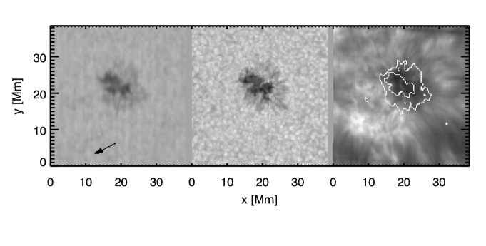
Figure 1: Intensity images created from TIP (left) and Hinode (middle) scans and the line core image of the Ca ii 854.2 nm line. White contours show the umbral and penumbral boundary of the TIP data. The arrow points towards disk center.

Sunspots are usually surrounded by a moat flow, an outward flow first detected by ?. At the outer boundary, the moat is separated from neighboring supergranules by the magnetic network. This flow is sometimes considered as an extension of the Evershed flow. ? obtained evidence for the continuation of the Evershed flow beyond the sunspot boundary even connected with supersonic velocities. ? found that there is no moat flow where the umbra reaches the outer spot boundary without a penumbra in between.

2 Observations and data processing

The small decaying sunspot in active region NOAA 11277 was observed on September 2, 2011 with the Vacuum Tower Telescope (VTT) on Tenerife and the Japanese Hinode satellite (?). In addition, we use data from the Helioseismic and Magnetic Imager (HMI, ???) on board the Solar Dynamics Observatory (SDO). The spot was located at 19^∘N and 30^∘W ($\vartheta$=31^∘).

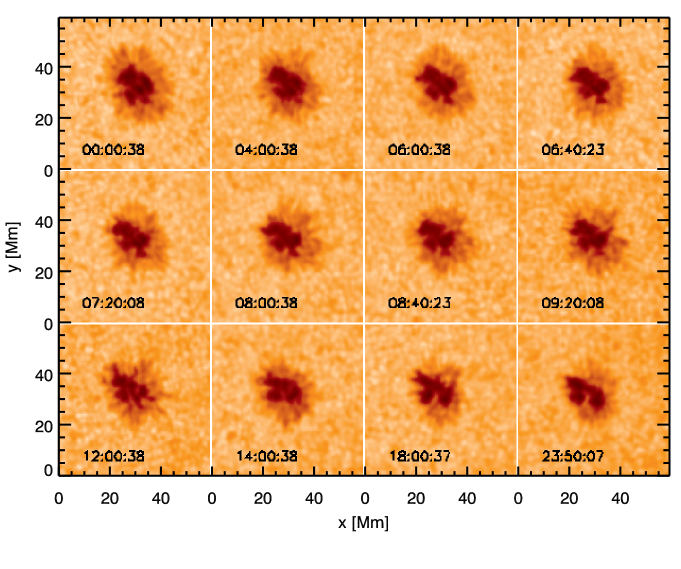
Figure 2: Intensity images from HMI/SDO showing the evolution of the spot on September 2, 2011.

At the VTT, we used the Tenerife Infrared Polarimeter 2 (TIP, ?) attached to the spectrograph to scan a map of the sunspot. We selected the spectral lines Fe i 1078.3 nm and Si i 1078.6 nm, which both split into Zeeman triplets with an effective Landé factor of 1.5. The scan consists of 150 steps with a 0^′′. 36 spacing. Four independent exposures with different states of the ferro-electric liquid crystals are required to obtain the full Stokes-vector, and we accumulated eight cycles. A single exposure took 250 ms, thus, about 10 s were needed per scan step. The scan was started at 08:09 UT and lasted 26 min. In addition to TIP, we mounted a CCD-camera centered on the line Ca ii 854.2 nm (see ?). Because this detector could not be synchronized with the polarimeter and has a low sensitivity at this wavelength, we integrated over 7.5 s. The image was stabilized by the Kiepenheuer Adaptive Optics System (KAOS, ?). A continuum image recombined from the TIP scans and a core image from the ionized calcium line are given in Fig. 1 together with the corresponding area covered by the Hinode scans.

The spot was in its decaying phase as shown in Fig 2, which displays selected HMI intensity images. The total series consists of 144 measurements taken every 10 min during September 2. At 00:00 UT, the umbra was still completely surrounded by a penumbra, while the umbra was already irregular but still continuous. During the time of the spectropolarimetric observations, the penumbra had almost disappeared on the eastern side. Later, the umbra split into two parts.

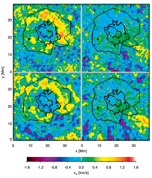
Figure 3: Horizontal velocities derived from LCT. The left column displays the radial component, the right column exhibits the tangential component. The upper panels show results from the Ca ii H filtergrams and the lower ones those from G-band. White contours show the boundary of the umbra, black contours the outer edge of the penumbra and the moat. Positive values indicate radial velocities away from the spot or counterclockwise tangential motions.

With the Hinode satellite we used the spectropolarimeter (HSP, ?) to take another map of the full Stokes-vector in the lines Fe i 630.15 nm and Fe i 630.25 nm. This map was started at 07:34 UT covering an area of 123^′′ $\times$ 123^′′ with 400 steps and a spacing of 0^′′. 3. In addition, we took filtergrams in Ca ii H and G-band every 32 s with the Broad-band Filter Imager (BFI) of the Solar Optical Telescope (SOT, ?). These filtergrams cover an area of 111^′′ $\times$ 111^′′  with a pixel size of 0^′′. 11 $\times$ 0^′′. 11. Such images were obtained over a period of three hours.

Strength and orientation of the magnetic field, and Doppler velocities from the photospheric lines were derived with the code Stokes Inversion based on Response functions (SIR, ?). We performed the inversions separately for the four spectral lines and considered the magnetic field and velocity to be height independent at least for the height range where the line profiles are affected by these quantities. Only the temperature was height dependent with three nodes. In preparation of the inversions, we subtracted 8% undispersed straylight from the TIP data and kept the amount of dispersed straylight fixed at 5% (typical VTT values, see ?). The magnetic azimuth ambiguity was resolved assuming that there is an azimuth center in the spot. This approach was sufficient for the TIP data. For the spatially more extended maps obtained with Hinode, we applied in addition the minimum energy code of ?. The coordinate system of the magnetic field was then rotated to the local reference frame. Finally, we corrected the geometrical foreshortening with the method described by ?.

3 Results

3.1 Velocity fields

The time series of Hinode filtergrams in Ca ii H and G-band were the base for a local correlation technique analysis (LCT) using the tools of ?. In Fig 3, we separate the horizontal velocities into a radial and a tangential component with respect to the center of the spot, as presented before by ?.

The moat flow is well visible around the spot, and it reaches a distance of another spot radius. This extension is less than the one investigated by ?, but still within the range given by ?. Velocities decrease from about 1000 m s^-1 at the penumbral boundary to about 200 m s^-1 at the outer edge of the moat. The moat flow is clearly detectable also on the side where the penumbra disappeared, but velocities close to the umbra are much smaller than on the opposite side of the spot. The tangential component is small inside the moat. Beyond the moat, the signature of the supergranulation becomes visible. The nearest neighboring supergranules cause a ring of velocities towards the spot, while an alternating pattern can be seen in the tangential component.

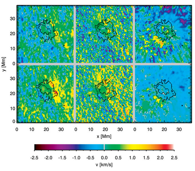
Figure 4: Doppler velocities from TIP (left, Si: upper panel, Fe: lower panel), from HSP (middle, Fe 630.15 top, Fe 630.25 bottom) and the infrared Ca line (right, line minimum top, bisector bottom). The chromospheric Ca ii IR velocities have been reduced by a factor of five to fit onto the same scale bar. Negative (blue) values correspond to blueshifts.

From the spectropolarimetric data, we also obtained Doppler velocities during the inversion process. To the core of the Ca ii 854.2 nm line, we applied a polynomial fit of fourth degree and calculated its minimum position, which gives us the velocity. In addition, we derived the bisector velocity at 0.275 of the continuum intensity. The line-of-sight velocities are shown in Fig 4. The Evershed effect is rather confined to deep photospheric layers. We see positive velocities outside the spot on the limb side, and a dominance of negative values on the center side. These velocities and their extensions are in agreement with the moat flow found by LCT. The most pronounced feature in the chromosphere is a downflow of more than 10 km s^-1 next to the spot on the center side. This downflow has no obvious counter part in photospheric layers. On the limb side, we see negative velocities, which are probably related to the inverse Evershed effect in the chromosphere.

3.2 The magnetic field

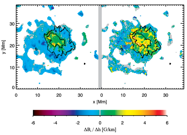
Figure 5: Gradients of the vertical magnetic field derived from the difference method from TIP (left) and Hinode (right) data.

The height dependence of $B_{\rm z}$ was derived in two different ways. The first method was to take the difference of $B_{\rm z}$ from two spectral lines divided by their height difference (difference method). To estimate the height difference, we used the temperature maps obtained for log $\tau$ = 0 and interpolated between the formation heights of the lines in a quiet-Sun atmosphere (Harvard Smithsonian Reference Atmosphere, ?) and in the umbral model M4 of ?. For the two iron lines from HSP, the height differences obtained this way are close to the 64 km determined by ? in the quiet Sun. This method was performed for the two TIP lines and the two HSP lines. The results for $\Delta B_{z}/\Delta z$ are displayed in Fig. 5.

The spot had a negative polarity, therefore $B_{\rm z}$ is negative, and a decrease of $|B_{\rm z}|$ with height appears as a positive number. In the umbra, we encounter a decrease of $|B_{\rm z}|$ by about 1 G km^-1 for the TIP data. Only close to the penumbral boundary, some locations exhibit up to 5 G km^-1. The decrease is much stronger for the HSP data. Here, we find values around 3 G km^-1 and more locations with about 5 G km^-1. In the penumbra, we find an increase of $|B_{\rm z}|$ for the TIP data, while the HSP data still exhibit a decrease. A possible explanation can be that Fe i 1078.3 nm is formed in deep layers, and the penumbral magnetic field might reside already above these layers.

The second method (derivative method) made use of the condition:

$$\rm{div}{\bf B}=\frac{\partial B_{x}}{\partial x}+\frac{\partial B_{y}}{\partial y}+\frac{\partial B_{z}}{\partial z}=0$$

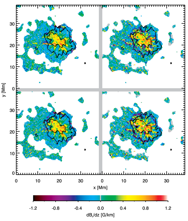
Figure 6: Vertical derivatives of the vertical component of the magnetic field strength derived from ${\rm div}{\bf B}=0$ for Si i 1078.6 nm (upper left), Fe i 1078.3 nm (lower left), Fe i 630.15 nm (upper right), and Fe i 630.25 nm (lower right).

This equation states that the vertical derivative must be compensated by the horizontal ones. The horizontal derivatives are determined from the difference of the values in the neighboring pixels (?). Such vertical derivatives were determined for all four lines and are shown in Fig. 6. With this method, we find maximum values of about 1 G km^-1 for ${\partial B_{z}}/{\partial z}$ from all four lines in the umbra, but also in some locations in the penumbra. For the outer penumbra, we encounter the opposite sign for this derivative. These results are in a good agreement with difference results obtained from the TIP data, while there are discrepancies for the HSP data. Remarkable is the fine structure seen in the HSP results, indicating the importance of high spatial resolution to obtain proper results from this method.

4 Discussion and Conclusions

The problem of the discrepancy between different methods to determine the height dependence of the magnetic field still exists, but there are indications that it becomes smaller with higher spatial resolution. Nevertheless, the difference method yields high values for the HSP data, but especially for these lines, the height differences are reliable. It would be much easier to argue that the formation layers of the TIP lines are not accurate enough, because the two lines are formed close to each other in the umbra, and it could be that they are closer together than estimated, resulting in a larger height gradient. A correct determination of the height dependence of the magnetic field might be provided in the near future by extending the geometric height scale algorithm of ? to an entire sunspot. So far, this method has been applied only to a small region of a sunspot. The spot is surrounded by an outward moat flow, as it is clearly visible from the LCT analysis. Photospheric Doppler shifts show opposite signs on both sides of the spot, and they can be interpreted as an outward flow, too. The extension of the moat is about one radius of the spot, in agreement with previous investigations, (e.g. ?). We still detect the moat flow on the side where the penumbra already disappeared, but more pronounced in the outer moat. This finding agrees with ?, but disagrees with the results of ?. Probably one has to distinguish between cases where a penumbra did not form because of the presence of another spot or pore of the same polarity (?) and cases where the penumbra disappears because the spot is decaying. In the chromosphere, the Doppler shifts have the opposite direction and exhibit the inverse Evershed effect. Remarkable is a downflow of more than 10 km s^-1 close to the spot which has no photospheric counterpart.

With the next generation of solar telescopes that are going into operation now, the New Solar Telescope at the Big Bear Solar Observatory (?) and GREGOR solar telescope at Tenerife (?) a big step towards better resolution will be done, and that will shed more light on the problems investigated in this contribution.

References

References

- Balthasar, H.: 2006, A&A 449, 1169.
- Balthasar, H. and Gömöry, P.: 2008, A&A 488, 1085.
- Balthasar, H. and Muglach, K.: 2010, A&A 511, A67.
- Balthasar, H. and Schmidt, W.: 1993, A&A 279, 243.
- Beck, C., Rezaei, R., and Fabbian, D.: 2011, A&A 535, A129.
- Beck, C., Rezaei, R., and Puschmann, K. G.: 2012, A&A 544, A46.
- Cao, W., Gorceix, N., Coulter, R. et al.: 2010, Astron. Nachr. 331, 636.
- Collados, M., Lagg, A., Díaz García, J.J. et al.: 2007,in: P. Heinzel, I. Dorotovič, R.J. Rutten (eds.), The physics of chromospheric plasmas ASPCS 368, 611.
- Couvidat,S., Schou, J., Shine, R. A. et al.: 2012, Sol. Phys. 275, 285.
- Deng, N., Choudhary, D. P., Tritschler, A. et al.: 2007,ApJ 671, 1013.
- Faurobert, M., Aime, C., Périni, C. et al.: 2009, A&A 507, L29.
- Gingerich, O., Noyes, R. W., Kalkofen, W., and Cuny, Y.: 1971, Sol. Phys. 18, 347.
- Hagyard, M. J., Teuber, D., West, E. A. et al.: 1983, Sol. Phys. 84, 13.
- Hofmann, A. and Rendtel, J.: 1989, Astron. Nachr. 310, 61.
- Ichimoto, K. Lites, B. W., Elmore, D. et al.: 2008, Sol. Phys. 249, 233.
- Kollatschny, W., Stellmacher, G., Wiehr, E., and Falipou, M. A.: 1980, A&A 86, 245.
- Kosugi, T., Matsuzaki,K., Sakao, T. et al.: 2007, Sol. Phys. 243, 3.
- Künzel, H.: 1969, Astron. Nachr. 291, 265.
- Leka, K. D., Barnes, G., Crouch, A. D. et al.: 2009, Sol. Phys. 260, 83.
- Martínez Pillet, V., Katsukawa, Y., Puschmann, K. G., and Ruiz Cobo, B.: 2009, ApJ 701, L79.
- Puschmann, K. G., Ruiz Cobo, B., and Martínez Pillet, V.: 2010, ApJ 720, 1417.
- Rempel, M.: 2011, ApJ 729, 5.
- Ruiz Cobo, B. and del Toro Iniesta, J.C.: 1992, ApJ 398, 375.
- Schmidt,W., von der Lühe, O., Volkmer, R. et al.: 2012, Astron. Nachr. 333, 796.
- Schou, J., Borrero, J. M., Norton, A. A. et al.: 2012b, Sol. Phys. 275, 327.
- Schou, J., Scherrer, P. H., Bush, R. I. et al.: 2012a, Sol. Phys. 275, 229.
- Sheeley, N. R.: 1972, Sol. Phys. 25, 98.
- Sobotka, M. and Roudier, T.: 2007, A&A 472, 277.
- Tsuneta, S., Ichimoto, K., Katsukawa, Y. et al.: 2008, Sol. Phys. 249, 167.
- Vargas Domínguez, S., Bonet, J. A., and Martínez Pillet, V. et al.: 2007, ApJ 600, L165.
- Verma, M. and Denker, C.: 2011, A&A 529, A153.
- Verma, M., Balthasar, H., Deng., N. et al.: 2012, A&A 538, A109.
- von der Lühe, O., Soltau, D., Berkefeld, T., and Schelenz, T.: 2003, Proc. SPIE 4853, 187.
- Wittmann, A.: 1974, Sol. Phys. 36, 29.