The spectrum of the relativistic radiation of electric charges and dipoles in their free falling into a black hole

Abstract

The free fall of electric charges and dipoles, radial and freely falling into the Schwarzschild black hole event horizon, was considered. Inverse effect of electromagnetic fields on the black hole is neglected. Dipole was considered as a point particle, so the deformation associated with exposure by tidal forces are neglected. According to the theorem, "the lack of hair"  of black holes, multipole magnetic fields must be fully emitted by multipole fall into a black hole. The spectrum of electromagnetic radiation power for these multipoles (monopole and dipole) was found. Differences were found in the spectra for different orientations of the falling dipole. A general method has been developed to find radiated electromagnetic multipole fields for the free falling multipoles into a black hole (including higher order multipoles — quadrupoles, etc.). The electromagnetic spectrum can be compared with observational data from stellar mass and smaller black holes.

1 Introduction

It is known Thorn1998 ; Frolov1998 , black hole has no "Hair", so all multipole moments of the electromagnetic fields disappear as the system of charges close to the horizon of the Schwarzschild black hole. Field problem for static point charge has been solved by Linet Linet1976 . In this problem it has been shown, in particular, that the field of a point charge close to the field of a charged black hole with the same charge, when the charge become close to the horizon. So all electric and magnetic multipoles moments should be radiated, when the charge (or a system of charges or currents) approach to the horizon of the Shwartzshild black hole.

Loss in the energy is defined essentially by bremsstrahlung, when monopole’s (unit charge) motion is accelerated. This is dipole radiation, since his power is inversely proportional to the $c^{3}$, and radiated field components are inversely proportional to the $c^{2}$.

The existence of dipole radiation is unobvious in the case when the massive dipole fall into black hole, because both charges of dipole are moving and accelerated in the same direction, and the signs of the charges are opposite. However, increasing curvature of space leads to the radiation of the dipole type (see section 4).

Complete analogy can be made with quadrupole radiation of gravitational waves in the orbital motion of the two masses (whose power is inversely proportional to ${c^{5}}$) in quadrupole approximation. In this case the signs of charges and masses are same, and velocities and accelerations are oppositely directed.

2 The law of motion of free falling particle

Let’s consider the radial free falling charge or electric dipole with mass $m$ on the Schwarzschild black hole horizon. Schwarzschild metric has the form :

$$ds^{2}=\left(1-\frac{r_{g}}{r}\right)dt^{2}-\left(1-\frac{r_{g}}{r}\right)^{-1}dr^{2}-r^{2}\,(d\theta^{2}+\sin^{2}\theta\,d\varphi^{2}).$$ (1)

Here ${r_{g}=2M}$ is the radius of the horizon of the Shwartzshild black hole. As you know, rapidly moving charge radiates. There is no radiation in the local neighborhood of the charge in their own co-moving frame .

The acceleration of a massive particle is defined by well-known expressions in a rigid system of reference at rest with respect to the black hole (seeLandau1988 , §87):

$$\frac{du^{i}}{ds}=-\Gamma^{i}_{kj}u^{k}u^{j}.$$ (2)

Here $u^{i}$ is component of 4-velocity and ${\Gamma^{i}_{kj}}$ are Christoffel symbols. We have for a Schwarzschild black hole (see Landau1988 , §100, 102) :

$$\Gamma^{r}_{tt}(r)=\frac{r_{g}}{2r^{2}}(1-r_{g}/r)\,,\quad\Gamma^{r}_{rr}(r)=-\frac{r_{g}}{2r^{2}(1-r_{g}/r)}\,,\quad{\dot{r}}_{e}=-\left(1-\frac{r_{g}}{r_{e}}\right)\sqrt{\frac{r_{g}/r_{e}-r_{g}/r_{0}}{1-r_{g}/r_{0}}},\,\,$$ (3)

$$v^{2}(r_{e})\equiv({\dot{r}}_{e})^{2}\frac{|g_{rr}|}{g_{tt}}=\frac{r_{g}/r_{e}-r_{g}/r_{0}}{1-r_{g}/r_{0}}\,,\quad u^{t}(r_{e})=\frac{\sqrt{1-r_{g}/r_{0}}}{1-r_{g}/r_{e}},\quad u^{r}(r_{e})=-\sqrt{r_{g}/r_{e}-r_{g}/r_{0}}\,.\,\,$$ (4)

Here ${r_{e}(t)}$ is the radius of the particle, ${r_{0}}$ is the radius at which the falling of the particle has been started and ${v(t)}$ is a three-dimensional velocity of the particle in the Schwarzschild coordinates.

The law of motion ${t(r_{e})}$ of the test particle is noticed in many papers (Frolov1998 , §2.4), which is free falling in the Schwarzschild field by radial trajectory from an infinite radius:

$$\frac{t(r_{e})}{r_{g}}=const-\frac{2}{3}\left(\frac{r_{e}}{r_{g}}\right)^{3/2}-2\sqrt{\frac{r_{e}}{r_{g}}}+\ln\left[\frac{\sqrt{r_{e}/r_{g}}+1}{\sqrt{r_{e}/r_{g}}-1}\right].$$ (5)

We need a similar law for a fall from a finite radius $r_{0}$.

The original formula is :

$$t(r_{e})=\sqrt{r_{e}(r_{0}-r_{e})(r_{0}/r_{g}-1)}+\frac{(r_{0}+2r_{g})\sqrt{r_{0}/r_{g}-1}}{2}\cdot\arccos\left(\frac{2r_{e}}{r_{0}}-1\right)+$$

$$+r_{g}\cdot\ln\left[\frac{2\sqrt{r_{e}(r_{0}-r_{e})(r_{0}/r_{g}-1)}+r_{0}+r_{e}(r_{0}/r_{g}-2)}{r_{0}(r_{e}/r_{g}-1)}\right].$$ (6)

So the initial conditions correspond to ${t{(r_{e}=r_{0})}=0}$.

Let’s imagine that there are clocks showing Schwarzschild time $t$ along the entire trajectory of the falling particle. Time ${\Delta t+\Delta t_{1}}$ passed as long as the light signal from the clock (which the particle flies by) reaches the observer. The time interval ${\Delta t}$ is the distance between the particle (when the particle flies past the clock) and its initial location (at the radius $r_{0}$). The time interval ${\Delta t_{1}=const}$ corresponds to the distance between the initial radius $r_{0}$ and a distant observer.

According to Landau1988 , §101 for period ${\Delta t}$ we have

$$\Delta t=r_{0}-r_{e}+r_{g}\ln\left[\frac{r_{0}-r_{g}}{r_{e}-r_{g}}\right].$$ (7)

It is assumed here and below, that the distant observer is almost on the same line, as the particle. Dependence on a small angle ${\theta<<\pi}$ can be negleted (in linear approximation) between radius vectors of the observer and of the particle in the formula (7).

Measurement of fall velocity of the particle by a distant observer must be described by time ${T(r_{e})\equiv t+\Delta t+\Delta t_{1}}$:

$$T(r_{e})=\sqrt{r_{e}(r_{0}-r_{e})(r_{0}/r_{g}-1)}+\frac{(r_{0}+2r_{g})\sqrt{r_{0}/r_{g}-1}}{2}\cdot\arccos\left(\frac{2r_{e}}{r_{0}}-1\right)+$$

$$+r_{g}\cdot\ln\left[\frac{2\sqrt{r_{e}(r_{0}-r_{e})(r_{0}/r_{g}-1)}+r_{0}+r_{e}(r_{0}/r_{g}-2)}{r_{0}(r_{e}/r_{g}-1)}\right]+r_{0}-r_{e}+r_{g}\ln\left[\frac{r_{0}-r_{g}}{r_{e}-r_{g}}\right]+const.\quad$$ (8)

Falling particle reach the horison in infinite time due to the logarithms in (6), (7) and (8).

Let’s introduce required notations:

$$a\equiv\sqrt{1-r_{g}/r_{e}},\quad b\equiv\sqrt{r_{g}/r_{e}-r_{g}/r_{0}},\quad c_{1}\equiv\sqrt{1-r_{g}/r_{0}}\,.$$ (9)

We have according to expressions (6) and (7):

$$\frac{dT}{dr_{e}}=\frac{1}{\dot{r}_{e}}-\frac{1}{1-r_{g}/r_{e}}=-\frac{b+c_{1}}{a^{2}b},$$ (10)

$$\beta(r_{e})\equiv\frac{dr_{e}}{dT}=-\frac{a^{2}b}{b+c_{1}}.$$ (11)

It is important to note, that ${\beta=0}$ for ${r_{e}=0}$ and ${r_{e}=r_{g}}$ (as well as for the quantity ${\dot{r}_{e}}$).

Physical meaning of the $\beta$ is observable (by a distant observer) velocity of the falling particle.

3 Spectral density of radiation

We use different method, than in the work Zerilli1970 ; Davis1971 ; Teukolsky1972 ; Yakovlev1975 ; Dymnikova1977 , to calculate the spectral density of the electromagnetic radiation.

The spectral density of the electromagnetic radiation from the radial current (which flows along ${\theta_{e}=0}$) is given by (Landau1988 , §66):

$$d{\cal E}_{\rm w}=-\frac{{\bf\hat{E}_{\rm w}^{\theta}}{\bf\hat{H}_{\rm w}^{\varphi}}}{4\pi^{2}}\cdot r^{2}\cdot do\cdot d{\rm w}\,,\quad do\equiv 2\pi\sin\theta\,d\theta\,.$$ (12)

Here ${{\bf\hat{E}_{\rm w}^{\theta}}({\rm w})}$ and ${{\bf\hat{H}_{\rm w}^{\varphi}}({\rm w})}$ are spectral densities of the physical components of electric and magnetic fields, which are orthogonal to the direction of wave propagation (at infinity); ${{\rm w}\equiv k_{t}}$ — the time component of the 4D null vector of photon $k_{j}$, and the components $k_{t}$ and $k_{\theta}$ are integrals of motion for each of the emitted photon.

General relativistic generalization of this formula is:

$$d{\cal E}_{\rm w}=-\frac{({\bf{F}_{\rm w}^{\theta t}}\sqrt{|g_{\theta\theta}g_{tt}|})({\bf{F}_{\rm w}^{\theta r}}\sqrt{|g_{\theta\theta}g_{rr}|})}{4\pi^{2}}\cdot r^{2}\cdot do\cdot d{\rm w}.$$ (13)

The expression (13) at infinity (far from the black hole) can be rewritten using that components of the electric and magnetic fields are equal by magnitude in the electromagnetic wave:

$$d{\cal E}_{\rm w}=-\frac{|{\bf{F}_{\rm w}^{\theta t}}|^{2}}{4\pi^{2}}\cdot r^{4}\cdot do\cdot d{\rm w}=-\frac{|{\bf{F}_{\rm w}^{\theta r}}|^{2}}{4\pi^{2}}\cdot r^{4}\cdot do\cdot d{\rm w}.$$ (14)

Thus radiated Fourier components of the field ${{\bf{F}_{\rm w}^{\theta t}}}$ and ${{\bf{F}_{\rm w}^{\theta r}}}$ at infinity must be inversely proportional to the square of the distance in order to satisfy the condition of energy conservation of electromagnetic waves.

The total energy radiated to infinity can be obtained either by integrating over frequency of expression (14), or by integration of the Poynting vector over time.

Spectral density tensor components ${{\bf{F}_{\rm w}^{mn}}}$ of the electromagnetic field and the contravariant components of the electromagnetic field ${F^{mn}}$ are associated with each other:

$${\bf{F}_{\rm w}^{mn}}=\int\limits_{-\infty}^{+\infty}F^{mn}\,\exp{\left[+i{\rm w}t\right]}\,dt,$$ (15)

$$F^{mn}=\frac{1}{2\pi}\int\limits_{-\infty}^{+\infty}{\bf{F}_{\rm\Omega}^{mn}}\,\exp{\left[-i\Omega t\right]}\,d\Omega.$$ (16)

Thus the spectral densities are obtained from the field components by the usual Fourier transform.

Because we assume, that beginning of the fall of the particle is the time ${t=0}$ for a distant observer, in this moment the radiation field must be absent (${F^{mn}_{\makebox{\scriptsize rad.}}=0}$ for ${t<0}$). This corresponds to half of the sum of the even and odd components of the radiation field, provided that the components we believe matching in absolute value.

(${|F^{mn}_{\makebox{\scriptsize rad.even.}}|=|F^{mn}_{\makebox{\scriptsize rad.odd.}}|=|F^{mn}_{\makebox{\scriptsize rad.}}|}$).

Then the Fourier transformation of (15)-(16) for the radiation fields can be rewritten as:

$${\bf{F}_{\rm w}^{mn}}=\int\limits_{0}^{\infty}F^{mn}\,\frac{1}{2}\left(\sin\left[{\rm w}t\right]+\cos\left[{\rm w}t\right]\right)\,dt=\int\limits_{0}^{\infty}F^{mn}\,\frac{1}{\sqrt{2}}\cos\left[{\rm w}t-\frac{\pi}{4}\right]\,dt,$$ (17)

$$F^{mn}=\frac{1}{4\pi}\int\limits_{0}^{\infty}{\bf{F}_{\rm\Omega}^{mn}}\,\left(\sin\left[\Omega t\right]+\cos\left[\Omega t\right]\right)\,d\Omega=\frac{\sqrt{2}}{4\pi}\int\limits_{0}^{\infty}{\bf{F}_{\rm\Omega}^{mn}}\,\cos\left[\Omega t-\frac{\pi}{4}\right]\,d\Omega.$$ (18)

In these formulas the sine corresponds to the odd component and the cosine corresponds to the even component of the radiation.

4 Radiation of a charge

We use the second pair of general relativistic Maxwell equations to find components of the spectral density ${{\bf{F}_{\rm w}^{mn}}}$ of the electromagnetic field (see Landau1988 , §90):

$$\partial_{i}\left(\sqrt{-g}F^{in}\right)=4\pi\sqrt{-g}j^{n}\,,\quad j^{n}(r,t,r_{0})=\sum\limits_{e}\frac{q_{e}\,u_{e}^{n}}{\sqrt{-g}\,u_{e}^{t}}\,\delta\left[r-r_{e}(t)\right]\cdot\delta(\theta)\cdot\delta(\varphi)\,.$$ (19)

Here ${\sqrt{-g}=r^{2}\sin\theta}$ and ${\delta\left[r-r_{e}(t)\right]}$ is delta function with a singularity at the point, where it is the charge at time $t$.

If ${r>r_{0}}$, the right side of equation (19) is always zero (4-vector current ${j^{n}=0}$), so we obtain following result by integrating of component $j^{t}$ of equation (19) over $\theta$ in ${[0,\,\theta]}$:

$$\int\limits_{0}^{\theta}\partial_{r}\left(\sqrt{-g}F^{rt}\right)\,d\theta+\sqrt{-g}F^{\theta t}=0$$ (20)

We rewrite (20) in the linear approximation in the small angle ${\theta<<\pi}$ as :

$$r^{2}F^{\theta t}=-\frac{\theta}{2}\partial_{r}\left[r^{2}F^{rt}\right]=\frac{\theta}{2}\partial_{r}\left[r^{2}F_{rt}\right]=\frac{\theta}{2}\partial_{r}\left[r^{2}(\partial_{r}A_{t}-\partial_{t}A_{r})\right]$$ (21)

Here $A_{i}$ is a 4-vector of the electromagnetic field of a falling charge in the stationary reference frame of a distant observer. Falling particle moves with a 4-speed $U^{i}$ relatively distant observer. Therefore expression (11) helps us to find the form of $U^{i}$ :

$$U^{i}\to\left\{\frac{1}{\sqrt{1-\beta^{2}}},\,\frac{\beta}{\sqrt{1-\beta^{2}}},\,0,\,0\right\}$$ (22)

Here and below the arrow indicates the limit as ${r/r_{g}\to\infty}$.

We use two invariants to find the components $A_{t}$ and $A_{r}$ in the frame of distant observer : ${inv_{1}=(A_{i}U^{i})=\tilde{A}_{t}}$ and ${inv_{2}=(A_{i}A_{j}g^{ij})=(\tilde{A}_{t})^{2}}$. Here ${\tilde{A}_{t}}$ is the only non-zero component of 4-vector ${\tilde{A}_{i}}$ of the electromagnetic field in the free falling frame reference associated with the particle. The expression for ${\tilde{A}_{t}}$ is known from work Linet1976 :

$$\tilde{A}_{t}=\frac{q_{e}}{rr_{e}}\left[\frac{(r-M)(r_{e}-M)-M^{2}\cos\theta}{\sqrt{(r-M)^{2}+(r_{e}-M)^{2}-M^{2}-2(r-M)(r_{e}-M)\cos\theta+M^{2}\cos^{2}\theta}}+M\right]$$ (23)

Here ${M=r_{g}/2}$ is the mass of the Schwarzschild black hole. In the linear approximation respect to the angle $\theta$ we obtain :

$$\tilde{A}_{t}{}_{(\theta=0)}=\frac{q_{e}(r-r_{g})}{r(r-r_{e})}\to\frac{q_{e}}{r}.$$ (24)

This shows that the required asymptotic of capacity has form of the Coulomb field in the free falling co-moving frame of reference. This essential and logical result is a consequence of the local inertial frame of reference in the falling "Einstein’s elevator."

Then we obtain the required components with omitting all intermediate calculations:

$$A_{t}=U_{t}\tilde{A}_{t}\to\frac{q_{e}}{r}\cdot\frac{1}{\sqrt{1-\beta^{2}}},$$ (25)

$$A_{r}=U_{r}\tilde{A}_{t}\to-\frac{q_{e}}{r}\cdot\frac{\beta}{\sqrt{1-\beta^{2}}}.$$ (26)

Expression (21) can be written in the limit ${r/r_{g}\to\infty}$ as :

$$F^{\theta t}\to-\frac{\theta}{2r^{2}}\cdot\partial_{r}\left[r^{2}\partial_{t}A_{r}\right]\to-\frac{\theta q_{e}}{2r^{2}}\cdot Z\,,\quad Z\equiv\frac{d}{dt}\left[\frac{\beta}{\sqrt{1-{\beta}^{2}}}\right]\,.$$ (27)

Here ${F^{\theta t}}$ is the tangential electric field of the radiation of a point charge when it is in the distance ${r_{e}}$ from the black hole. It should be noted that this field is dipolar, since it is proportional to $r_{g}$ and inversely proportional to the square of the speed of light.

We will get from (27) using the derivative with respect to time:

$$Z=\frac{\dot{r}_{e}}{\left(1-{\beta}^{2}\right)^{3/2}}\cdot\frac{\partial{{\beta}}}{\partial r_{e}}=-\frac{r_{g}a^{2}(b+c_{1})[a^{2}c_{1}-2b^{2}(b+c_{1})]}{2c_{1}r_{e}^{2}[(b+c_{1})^{2}-a^{4}b^{2}]^{3/2}}$$ (28)

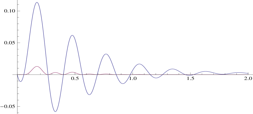
Figure 1: Radial fall of a point charge $q_{e}$ from radius ${r_{0}=5r_{g}}$ into the black hole.
Curve with variable sign and greater amplitude is the spectral density (Fourier transform) of the radiation field ${{\bf F_{\rm w}^{\theta t}}}$ of the argument ${({\rm w}r_{g})}$ in units ${\left[q_{e}\theta/r^{2}\right]}$.
Curve with fixed sign and lower amplitude is the square of ${{\bf F_{\rm w}^{\theta t}}}$, which is the power spectrum of electromagnetic radiation (14).

We obtain by substituting (27) and (28) in the Fourier transform (17):

$${\bf{F}_{\rm w}^{\theta t}}=\int\limits_{0}^{\infty}\frac{\cos\left[{\rm w}t-\frac{\pi}{4}\right]}{\sqrt{2}}\,F^{\theta t}\,dt=-\frac{\theta q_{e}}{r^{2}}\int\limits_{0}^{\infty}\frac{\cos\left[{\rm w}t-\frac{\pi}{4}\right]}{2\sqrt{2}}\,\partial_{t}\left[\frac{\beta}{\sqrt{1-{\beta}^{2}}}\right]\,dt$$ (29)

We obtain by replacing in (29) integration variable: ${dt=dr_{e}/{\dot{r}_{e}}}$, according to (9) for the spectral density of the radiation field:

$${\bf{F}_{\rm w}^{\theta t}}=-\frac{\theta q_{e}}{r^{2}}\int\limits_{0}^{\infty}\frac{{\rm w}\,\sin[{\rm w}t-\frac{\pi}{4}]\,\beta}{2\sqrt{2}\sqrt{1-{\beta}^{2}}}\,dt=\frac{\theta q_{e}}{r^{2}}\int\limits_{r_{g}}^{r_{0}}\frac{{\rm w}\,c_{1}\,\sin\left[{\rm w}t(r_{e})-\frac{\pi}{4}\right]}{2\sqrt{2}\sqrt{(b+c_{1})^{2}-a^{4}b^{2}}}\,dr_{e}$$ (30)

We used here the integration by parts and we noted that ${\beta=0}$ in points ${r_{e}=0}$ and ${r_{e}=r_{g}}$. The function ${t(r_{e})}$ is given by expression (6).

Results obtained using (30) are shown in Figure 1. The spectral density of the radiation field of a charge is shown below. Here we use posibility of integration (29) in parts, according to the expression (26) and (30).

$${\bf{F}_{\rm w}^{\theta t}}=\frac{\theta{\rm w}}{r}\cdot{\bf A_{r{\rm w}}}$$ (31)

Here ${\bf A_{i{\rm w}}}$ is the Fourier transform of the retarded vector potential for the field of the charge. It corresponds to the usual definition of the Fourier components of the radiation field (${{\bf|\hat{E}_{\rm w}^{\theta}|}={\rm w}\sin\theta|\vec{\bf A}_{\rm w}|}$ — see Landau1988 , §66), and it is possible by ability of integration by parts in (29). But dipole field representation in the form (31) is not possible, as it will be shown in the next section.

5 Dipole radiation

The value of the dipole is defined as: ${d_{0}\equiv q_{e}l_{0}=const}$. We assume the dipole as point particle (${l_{0}<<<r_{g}}$) and neglect the deformation related to effects of tidal forces. We denote the radius of the dipole location: ${r_{d}\equiv(r_{1}+r_{2})/2}$, then respectively replace ${r_{e}\to r_{d}}$ in all expressions for dipoles.

5.1 Transverse orientation of the dipole

First we choose the orientation of the dipole across the radius (the simplest case). Then ${l_{0}=r_{d}\Delta\theta_{d}}$, so the expression (27) for the tangential electric field of the dipole radiation in this case will be rewritten as :

$$F^{\theta t}_{d_{\perp}}=\Delta\theta_{d}\cdot\frac{\partial F^{\theta t}}{\partial\theta}=\frac{-d_{0}Z}{2r_{d}r^{2}}=\frac{d_{0}}{r^{2}}\cdot\frac{r_{g}a^{2}(b+c_{1})[a^{2}c_{1}-2b^{2}(b+c_{1})]}{4c_{1}r_{d}^{3}[(b+c_{1})^{2}-a^{4}b^{2}]^{3/2}}$$ (32)

The function ${F^{\theta t}_{d_{\perp}}{}_{(t,r)}}$ is the tangential electric field of the dipole radiation at the time of its location at a distance ${r_{d}}$ from the black hole (for transverse orientation).

Figure 2: Radial fall of a dipole from radius ${r_{0}=5r_{g}}$ on the black hole.
For transversely oriented dipole (top): variable sign curve with greater amplitude is the spectral density (Fourier transform) of the radiation field ${{\bf{F}_{\rm w{d_{\perp}}}^{\theta t}}}$ of the argument ${({\rm w}r_{g})}$, in units of ${\left[d_{0}/(r_{g}r^{2})\right]}$. Fixed sign curve with lower amplitude is the square of ${{\bf{F}_{\rm w{d_{\perp}}}^{\theta t}}}$, which is proportional to the power spectrum (14) of electromagnetic radiation.

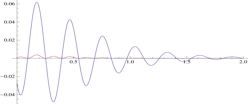
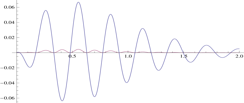
Figure 3: The same thing for longitudinally oriented dipole is ${{\bf{F}_{\rm w{d_{\parallel}}}^{\theta t}}}$, in units of ${\bf\left[d_{0}\theta/(r_{g}r^{2})\right]}$.

   

So the spectral density of the radiation field of a dipole takes the form in the transverse orientation:

$${\bf F_{{\rm w}d_{\perp}}^{\theta t}}=\int\limits_{0}^{\infty}\frac{F^{\theta t}_{d_{\perp}}\,\cos\left[{\rm w}t-\frac{\pi}{4}\right]}{\sqrt{2}}\,dt=\frac{d_{0}}{r^{2}}\int\limits_{r_{g}}^{r_{0}}\frac{r_{g}\,\cos[{\rm w}t(r_{d})-\frac{\pi}{4}]\,(b+c_{1})[a^{2}c_{1}-2b^{2}(b+c_{1})]}{4\sqrt{2}br_{d}^{3}[(b+c_{1})^{2}-a^{4}b^{2}]^{3/2}}\,dr_{d}\quad$$ (33)

Here the variable of integration was replaced with ${dt=dr_{d}/{\dot{r}_{d}}}$, as in the expression (30).

It is important to note that the dipole radiation is independent of $\theta$ in the linear approximation by the angle ${\theta<<\pi}$ in the case of the transverse orientation (since the radiation pattern of the dipole is located just in the transverse direction).

5.2 Longitudinal orientation of of the dipole

Now let’s choose the orientation of the dipole along the radius. Length of the dipole can be calculated using following formula taking into account the curvature of space:

$$l_{0}\approx[r_{2}(t)-r_{1}(t)]/\sqrt{1-r_{g}/r_{d}}$$ (34)

Hence it follows

$$\Delta r_{d}\equiv r_{2}(t)-r_{1}(t)=a\cdot l_{0}\,,\quad\Delta r_{0}=c_{1}\cdot l_{0}.$$ (35)

Here $\Delta$ denotes the change at constant time $t$, so differential must be zero:

$$dt=\frac{\partial t}{\partial r_{0}}\cdot\Delta r_{0}+\frac{\partial t}{\partial r_{d}}\cdot\Delta r_{d}=0.$$ (36)

Expression (27) for a dipole can be written as:

$$F^{\theta t}_{d_{\parallel}}=\Delta F^{\theta t}\equiv\frac{\partial F^{\theta t}}{\partial r_{0}}\cdot\Delta r_{0}+\frac{\partial F^{\theta t}}{\partial r_{d}}\cdot\Delta r_{d}=\left[\frac{\partial F^{\theta t}}{\partial r_{0}}-\frac{\partial F^{\theta t}}{\partial r_{d}}\cdot\frac{\partial t}{\partial r_{0}}\cdot{\dot{r}_{d}}\right]\cdot c_{1}\cdot l_{0}.$$ (37)

Similarly to the case of the transverse orientation of the dipole the spectral density of the radiation field for the dipole in the longitudinal orientation takes the form:

$${\bf{F}_{\rm w{d_{\parallel}}}^{\theta t}}=\int\limits_{0}^{\infty}\frac{F^{\theta t}_{d_{\parallel}}\,\cos\left[{\rm w}t-\frac{\pi}{4}\right]}{\sqrt{2}}\,dt=\frac{d_{0}\theta}{r^{2}}\int\limits_{r_{g}}^{r_{0}}\frac{c_{1}\,\cos\left[{\rm w}t(r_{d})-\frac{\pi}{4}\right]}{2\sqrt{2}}\cdot\left[\frac{\partial Z}{\partial r_{0}}-{\dot{r}_{d}}\cdot\frac{\partial t}{\partial r_{0}}\cdot\frac{\partial Z}{\partial r_{d}}\right]\,\frac{dr_{d}}{\dot{r}_{d}}\quad.$$ (38)

The derivatives necessary for calculation of the quadrature (with regard to the expression (28)) are given in Appendix (see (39), (40) and (41)).

Plots of the power spectrum for the transverse and longitudinal dipole orientations are shown in Figure 3 and Figure 3, respectively.

6 Discussion and conclusions

As shown in previous sections, the radiation both falling monopole and falling dipole ((32) and (37)) are dipolar, because radiated field components are proportional to $r_{g}$ (28), that is inversely proportional to $c^{2}$.

The total energy of the radiation received by integration over time of the Poynting vector is ${{\cal E}=\frac{1}{4\pi}\int\limits(F^{\theta t})^{2}r^{4}\,do\,dt}$. It is equal ${{\cal E}^{e}\approx 0.0016q_{e}^{2}/r_{g}}$ for the monopole and ${{\cal E}^{d}\approx 0.0007d_{0}^{2}/r_{g}^{3}}$ for the dipole, taking into account the angular distribution of power (see Ross1971 or Landau1988 , §67). In addition, the energy of the radiation exceeds their rest energy for the falling electrons in the field of black holes with a mass less than $10^{14}{g}$. It speaks about the infidelity of above calculations for radiation in the classical theory for primordial black holes (with a mass less than ${10^{14}}$ g). In these cases it is necessary to use other theory (quantum gravity).

Found spectrum of dipole radiation depends on the orientation of the dipole.

Wavelength characteristic $\lambda_{m}$ depends on the specific value of ${r_{0}}$ and on the orientation of the dipole at the maximum of the radiation. $\lambda_{m}$ is approximately ${20r_{g}}$, when ${r_{0}=5r_{g}}$. Therefore it’s possible to observe this radiation near the maximum for a relatively small black hole (with a mass ${M<\sim M_{\odot}}$). If you’ll try to observe this radiation at shorter wavelengths, spectral power decreases approximately as ${{\rm w}^{-4}}$ in the local maximum .

Since this radiation has a spectrum characteristic, it can be registered for the rare cases of falling magnetized planets (or asteroids) on black holes of stellar mass or even in rare cases, when pulsars fall into the black hole.

Aknowledgments

We are particularly grateful to K.A. Bronnikov for many useful discussions on the subject and for valuable comments.

This work was supported by RFBR, project codes: 12-02-00276-a, 11-02-00244-a, 11-02-12168-ofi-m-2011, Scientific School-2915.2012.2 "Formation of large-scale structure of the Universe and cosmological processes" Programme "Nonstationary Phenomena in the objects of the universe 2012"  and the Federal Target Program "Scientific and pedagogical Staff of Innovative Russia 2009-2013"   16.740.11.0460.

.1 APPENDIX: necessary for the integration of quadrature (38) expressions

We denote ${x\equiv r_{g}/r_{d}}$, ${y\equiv r_{g}/r_{0}}$ and give the necessary expressions:

$$\frac{\partial Z}{\partial r_{0}} = \frac{(x-1)^{2}x^{2}y^{2}}{4r_{g}^{2}(1-y)^{3/2}\sqrt{x-y}\left[1-x^{3}+x^{2}(y+2)-2xy+2\sqrt{(1-y)(x-y)}-y\right]^{5/2}}$$ (39)

$$\times \left[2x^{4}\sqrt{x-y}+x^{3}\left(2\sqrt{1-y}-7\sqrt{x-y}\right)\right.$$

$$+ \left.2\left(x^{2}-2x-15\right)y^{2}\left(\sqrt{x-y}+\sqrt{1-y}\right)+x^{2}\left(9\sqrt{x-y}-14\sqrt{1-y}\right)\right.$$

$$+ \left.y\left\{-x^{3}\left(\sqrt{x-y}+2\sqrt{1-y}\right)+x^{2}\left(2\sqrt{1-y}-\sqrt{x-y}\right)+x\left(29\sqrt{x-y}+42\sqrt{1-y}\right)\right.\right.$$

$$+ \left.\left.37\sqrt{x-y}+22\sqrt{1-y}\right\}-x\left(29\sqrt{x-y}+18\sqrt{1-y}\right)-7\sqrt{x-y}-2\sqrt{1-y}\right]$$

$$\frac{dt}{dr_{0}}=\frac{1-(x+1)y/(2x)+y^{2}}{\sqrt{(1-y)(x-y)}}+\frac{\sqrt{1-y}(2y+1)}{2\sqrt{x-y}}+\frac{3\arccos\left(2y/x-1\right)}{4\sqrt{y(1-y)}}$$ (40)

$$\frac{\partial Z}{\partial r_{d}} = \frac{x^{3}\left[(2-y)y(x-y)+2\sqrt{(1-y)(x-y)}+1-y\right]^{-1/2}}{4r_{g}^{2}\sqrt{(1-y)(x-y)}\left[(2-x)x(x-y)+2\sqrt{(1-y)(x-y)}+1-y\right]^{2}}$$ (41)

$$\times \left[2x^{6}\sqrt{x-y}-x^{5}\left(17\sqrt{x-y}+18\sqrt{1-y}\right)+x^{4}\left(8\sqrt{x-y}-26\sqrt{1-y}\right)\right.$$

$$- \left.4x^{3}\left(25\sqrt{x-y}+14\sqrt{1-y}\right)+16\left(x^{2}+4x-3\right)y^{3}\left(\sqrt{x-y}+\sqrt{1-y}\right)\right.$$

$$+ \left.x^{2}\left(62\sqrt{x-y}+78\sqrt{1-y}\right)+2y^{2}\left\{x^{4}\left(\sqrt{x-y}+\sqrt{1-y}\right)-x^{3}\left(25\sqrt{x-y}+29\sqrt{1-y}\right)\right.\right.$$

$$- \left.\left.x^{2}\left(79\sqrt{x-y}+91\sqrt{1-y}\right)+x\left(33\sqrt{x-y}+61\sqrt{1-y}\right)+22\sqrt{x-y}+10\sqrt{1-y}\right\}\right.$$

$$+ \left.y\left\{-x^{5}\left(\sqrt{x-y}+2\sqrt{1-y}\right)+12x^{4}\left(3\sqrt{x-y}+5\sqrt{1-y}\right)\right.\right.$$

$$+ \left.\left.\left.2x^{3}\left(50\sqrt{x-y}+71\sqrt{1-y}\right)-4x^{2}\left(3\sqrt{1-y}-26\sqrt{x-y}\right)-x\left(151\sqrt{x-y}+104\sqrt{1-y}\right)\right.\right.\right.$$

$$+ \left.\left.8\sqrt{x-y}+12\sqrt{1-y}\right\}+x\left(17\sqrt{x-y}-10\sqrt{1-y}\right)-4\sqrt{x-y}\right]$$

It is interesting that all these expressions are singular at the point ${r_{d}=r_{0}}$, but their combination in the formula (38), is finite.

References

• (1) Black Holes: The Membrane Paradigm (1998), K.S. Thorne, R.H. Price, D.A. Macdonald ed.
• (2) V.P. Frolov and I.D. Novikov, Black Hole Physics. Basic Concepts and New Developments (Kluver AP, 1998).
• (3) B.Linet, J. Phys. A 9, 1081 (1976).
• (4) L.D. Landau and E.M. Lifshitz, Field Theory (Moscow, Science, 1988).
• (5) F.J. Zerilli, Phys. Rev. D 2, 2141 (1970).
• (6) M. Davis, R. Ruffini, W.H. Press and R.H. Price, Phys. Rev. Lett. 27, 1466 (1971).
• (7) S.A. Teukolsky, Phys. Rev. Lett. 29, 1114 (1972).
• (8) D.G. Yakovlev, JETP 41, 179 (1975).
• (9) I.G. Dymnikova, Astrophysics and Space Science 51, 229 (1977).
• (10) D.K. Ross, Astron. Soc. Pacific 83, 633 (1971).