Normal and superconducting properties of LiFeAs explained in the framework of four-band Eliashberg Theory

Abstract

In this paper we propose a model to reproduce superconductive and normal properties of the iron pnictide LiFeAs in the framework of the four-band $s\pm$ wave Eliashberg theory. A confirmation of the multiband nature of the system rises from the experimental measurements of the superconductive gaps and resistivity as function of temperature. We found that the most plausible mechanism is the antiferromagnetic spin fluctuation and the estimated values of the total antiferromagnetic spin fluctuation coupling constant in the superconductive and normal state are $\lambda_{\rm tot}=2.00$ and $\lambda_{\rm tot,tr}=0.77$.

Recent ARPES measurements of iron superconductor LiFeAs report four slightly anisotropic gaps GapUmez . Their isotropic values at 8 K are given by $\Delta_{\rm 1}=5.0$ meV, $\Delta_{\rm 2}=2.6$ meV, $\Delta_{\rm 3}=3.6$ meV, $\Delta_{\rm 4}=2.9$ meV and the critical temperature for this compound is $T_{\rm c}=18$ K Tapp .

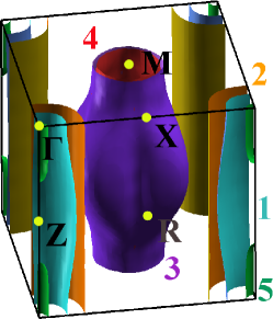
Figure 1: Fermi surface of LiFeAs computational .

FS	1	2	3	4	5	TOT
N(0)	0.556	0.646	0.616	0.370	0.039	2.228
$\omega_{p}^{\parallel ab}$	1.131	1.455	1.581	1.161	0.639	2.980
$\omega_{p}^{\parallel c}$	0.202	0.034	0.890	0.365	0.319	1.523

Table 1: Fermi Surface resolved Kohn Sham properties: the Fermi density of states $N(0)$ is given in states/spin/eV and plasma frequencies $\omega_{p}$ in eV. $ab$ label the in-plane and $c$ for the out-of-plane direction of the diagonals of the plasma tensor PDdolghi .

In an other work Us we disregarded the anisotropic part of the gap values and we tried to reproduce the experimental data in the framework of $s\pm$ wave multiband Eliashberg theory. At first, we calculated Us ; computational ; KS ; PBE ; espresso ; PDdolghi the Fermi surface, depicted in FIG. 1: Five different sheets are present, with two electron pockets centered near the M-point of the Brillouin zone and three hole pockets around the $\Gamma$-point. The 5-th sheet can be disregarded thanks to its low density of states and size Us as can be seen in TABLE 1. In this way a four-band s-wave Eliashberg model EE ; ema can be used and eight coupled equations for the gaps $\Delta_{i}(i\omega_{n})$ and the renormalization functions $Z_{i}(i\omega_{n})$ have to be solved. If $i$ is the band index (that ranges between $1$ and $4$) and $\omega_{n}$ are the Matsubara frequencies, the imaginary-axis equations are:

$$\omega_{n}Z_{i}(i\omega_{n}) = \omega_{n}+\pi T\sum_{m,j}\Lambda^{Z}_{ij}(i\omega_{n},i\omega_{m})N^{Z}_{j}(i\omega_{m})+$$ (1)

$$+\sum_{j}\big{[}\Gamma_{\rm ij}+\Gamma^{M}_{\rm ij}\big{]}N^{Z}_{j}(i\omega_{n})\,,$$

$$Z_{i}(i\omega_{n})\Delta_{i}(i\omega_{n}) = \pi T\sum_{m,j}\big{[}\Lambda^{\Delta}_{ij}(i\omega_{n},i\omega_{m})-\mu^{*}_{ij}(\omega_{c})\big{]}\times$$ (2)

$$\times\Theta(\omega_{c}-|\omega_{m}|)N^{\Delta}_{j}(i\omega_{m})$$

$$+\sum_{j}[\Gamma_{\rm ij}+\Gamma^{M}_{\rm ij}]N^{\Delta}_{j}(i\omega_{n})\,;$$

where $\Gamma_{\rm ij}$ and $\Gamma^{M}_{\rm ij}$ are the non magnetic and magnetic impurity scattering rates, $\Theta(\omega_{c}-|\omega_{m}|)$ is the Heaviside function and $\omega_{c}$ is a cutoff energy. Moreover, $\mu^{*}_{ij}(\omega_{\rm c})$ are the elements of the $4\times 4$ Coulomb pseudopotential matrix and $N^{\Delta}_{j}(i\omega_{m})=\Delta_{j}(i\omega_{m})/{\sqrt{\omega^{2}_{m}+\Delta^{2}_{j}(i\omega_{m})}}$, $N^{Z}_{j}(i\omega_{m})=\omega_{m}/{\sqrt{\omega^{2}_{m}+\Delta^{2}_{j}(i\omega_{m})}}$. Finally,

$$\Lambda^{Z}_{ij}(i\omega_{n},i\omega_{m})=\Lambda^{ph}_{ij}(i\omega_{n},i\omega_{m})+\Lambda^{sf}_{ij}(i\omega_{n},i\omega_{m})$$

$$\Lambda^{\Delta}_{ij}(i\omega_{n},i\omega_{m})=\Lambda^{ph}_{ij}(i\omega_{n},i\omega_{m})-\Lambda^{sf}_{ij}(i\omega_{n},i\omega_{m}).$$

Here the superscripts sf and ph mean “antiferromagnetic spin fluctuations” and “phonons”, respectively. In particular,

$$\Lambda^{ph,sf}_{ij}(i\omega_{n},i\omega_{m})=2\int_{0}^{+\infty}d\Omega\Omega\frac{\alpha^{2}_{ij}F^{ph,sf}(\Omega)}{(\omega_{n}-\omega_{m})^{2}+\Omega^{2}},$$

and the electron-boson coupling constants are defined as

$$\lambda^{ph,sf}_{ij}=2\int_{0}^{+\infty}d\Omega\,\frac{\alpha^{2}_{ij}F^{ph,sf}(\Omega)}{\Omega}.$$ (3)

The solution of eqs.(1) and (2) requires a huge number of input parameters, then drastic approximations, compatible with the goal of reproducing the essential physics of the problem, are necessary to make the model solvable. As for many other pnictides we assumed that Us : i) the total electron-phonon coupling constant is small Boeri ; ii) spin fluctuations mainly provide interband coupling Umma1 . This means that we can set $\lambda^{ph}_{ii}=\lambda^{ph}_{ij}=0$, $\mu^{*}_{ii}(\omega_{\rm c})=\mu^{*}_{ij}(\omega_{\rm c})=0$, i.e. the electron-phonon coupling constant and the Coulomb pseudopotential in first approximation compensate each other and $\lambda^{sf}_{ii}=0$ (only interband SF coupling) Umma1 . However, within these assumptions, we were not able to reproduce the observed gap values, and in particular the high value of $\Delta_{1}$. In order to solve this problem it is necessary to introduce an intraband coupling in the first band ($\lambda_{11}\neq 0$).
The final matrix of the electron-boson coupling constants becomes

$$\lambda_{ij}=\left(\begin{array}[]{cccc}\lambda_{11}&0&\lambda_{13}&\lambda_{14}\\ 0&0&\lambda_{23}&\lambda_{24}\\ \lambda_{31}=\lambda_{13}\nu_{13}&\lambda_{32}=\lambda_{23}\nu_{23}&0&0\\ \lambda_{41}=\lambda_{14}\nu_{14}&\lambda_{42}=\lambda_{24}\nu_{24}&0&0\\ \end{array}\right)$$ (4)

where $\nu_{ij}=N_{i}(0)/N_{j}(0)$ and $N_{i}(0)$ is the normal density of states at the Fermi level for the $i$-th band ($i=1,2,3,4$). We choose spectral functions with Lorentzian shape Umma1 ; Inosov i.e:

$$\alpha_{ij}^{2}F_{ij}(\Omega)=C_{ij}\big{\{}L(\Omega+\Omega_{ij},Y_{ij})-L(\Omega-\Omega_{ij},Y_{ij})\big{\}}$$ (5)

where $L(\Omega\pm\Omega_{ij},Y_{ij})=\frac{1}{(\Omega\pm\Omega_{ij})^{2}+Y_{ij}^{2}}$ and $C_{ij}$ are normalization constants, necessary to obtain the proper values of $\lambda_{ij}$ while $\Omega_{ij}$ and $Y_{ij}$ are the peak energies and half-widths of the Lorentzian functions, respectively Umma1 . In all the calculations we set $\Omega_{ij}=\Omega_{ij}^{sf}=\Omega_{0}^{sf}=8$ meV Taylor , and $Y_{ij}=Y_{ij}^{sf}=\Omega_{ij}^{sf}/2$ Inosov . The cut-off energy is $\omega_{c}=18\,\Omega_{0}^{sf}$ and the maximum quasiparticle energy is $\omega_{max}=21\,\Omega_{0}^{sf}$. Bandstructure calculations (see TABLE 1) provide information about the factors $\nu_{ij}$ that enter the definition of $\lambda_{ij}$. In the end the model contains five free parameters: The coupling constants $\lambda_{13},\,\lambda_{23},\,\lambda_{14},\,\lambda_{24}$ and $\lambda_{11}$. First of all we solved the imaginary-axis Eliashberg equations (1) and (2) (actually we continued them analytically on the real-axis by using the Padé approximant technique) and we fixed the free parameters in order to reproduce the gap values at low temperature. The large number of free parameters (five) may suggest that it is possible to find different sets that produce the same results. On the contrary, as a matter of fact, the predominantly interband character of the model drastically reduce the number of possible choices. At this point there are no more free parameters. We can calculate the critical temperature and it turns out to be very close to experimental one  Tapp : $T^{calc}_{c}=18.6$ K. In TABLE 2 the obtained results are summarized. The problem of this model is the necessity of a so large intraband term $\lambda_{11}$ in order to give a physical interpretation of the experimental data Us .

	$\lambda_{11}$	$\lambda_{tot}$	$\lambda_{13}$	$\lambda_{23}$	$\lambda_{14}$	$\lambda_{24}$	$\Delta_{1}$	$\Delta_{2}$	$\Delta_{3}$	$\Delta_{4}$	$T_{c}$
Exper.	-	-	-	-	-	-	5.0	2.6	3.6	2.9	18
Theor.	0.0	1.8	1.78	0.66	0.45	0.52	3.7	2.6	3.6	2.9	15.9
Theor.	2.1	2.0	1.15	0.80	0.45	0.30	5.0	2.6	3.6	2.9	18.6

Table 2: In the first row are shown the experimental data. The second row concerns the pure intraband case ($\lambda_{ii}=0.0$) while the third one concerns the case with a large intraband term ($\lambda_{11}=2.1$). The critical temperatures are given in K and the gap values in meV.

Regarding the normal state Heyer , the resistivity saturation at high temperature Kasahara suggests that the presence of several sheets in the Fermi surface also affects the normal state transport properties.
First of all we noticed (see FIG. 2) that at low temperature $\rho(T)\propto T^{\rm 2}$ and this could indicate that a non-phononic mechanism plays a relevant role in the physics of this compound Gur2D .
To begin with, we tried to fit the data within a one-band model Allen ; grim (see eq. (6) with $i=1$) where the phonon spectra has been taken from ref. BorisPH and the plasma energy has been obtained by first principle calculation (see TABLE 1). The transport coupling constant and the value of the impurities are considered as free parameters. The obtained values are reported in TABLE 3, in particular $\lambda_{\rm tr,tot}=0.32$ which is in agreement with the calculated value of the trasport electron-phonon coupling constant phonon . However, as can be seen in FIG. 2, within a one-band model (black dashed line) the experimental data cannot be reproduced.
Phenomenological model PhenModel proposed to explain saturation at high temperature generally assume the presence of parallel conductivity channels where one of them has a strong temperature dependence and another one is characterized by a temperature-independent contribution.

	$\lambda_{\rm tr,tot}$	$\lambda_{\rm tr,3}$	$\lambda_{\rm tr,4}$	$\gamma_{\rm 1}$	$\gamma_{\rm 2}$	$\gamma_{\rm 3}$	$\gamma_{\rm 4}$	$\Omega_{\rm 0}$
ph 1 band	0.32	-	-	0.90	-	-	-	-
ph 4 bands	0.14	0.44	0.10	5100	5100	0.65	550	-
sf 4 bands	0.77	1.70	1.70	164	164	4.87	1.52	47

Table 3: The first and second rows concern the phonon case while the third one concerns the case of the antiferromagnetic spin fluctuation spectral function. The $\gamma_{\rm i}$ and $\Omega_{\rm 0}$ are given in meV.

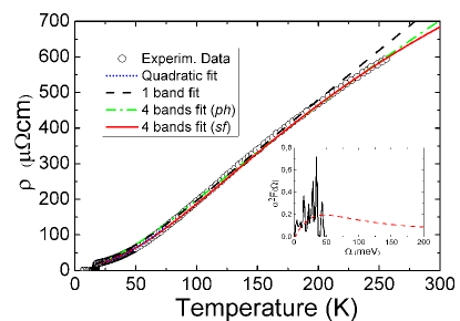
Figure 2: Temperature dependence of resistivity in LiFeAs. Experimental data and calculated fits are reported. The black dashed line comes from a single-band model. Within a four-band model two different cases have been considered, one is obtained with the phononic spectra (green dash-dotted line) and one with the antiferromagnetic spin fluctuation spectra (red solid line). The inset shows the two normalized spectral function that have been used, the phonon spectra (black solid line) and the antiferromagnetic spin fluctuation spectra (red dashed line)

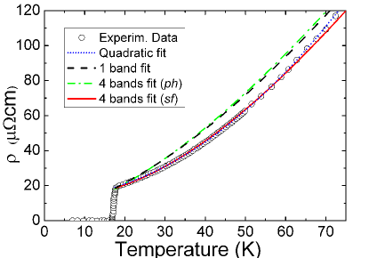
Figure 3: Magnification of the previous figure. Resistivity at low temperature.

In the wake of the model proposed for the superconducting state, we propose a multiband model MgB2 ; DolghiBaK for analyzing the resistivity data. We will examine two possible mechanism responsible of resistivity: Phonons and antiferromagnetic spin fluctuations. The theoretical expression of the resistivity as function of temperature MgB2 ; DolghiBaK is given by the equation:

$$\frac{1}{\rho_{\rm c}(T)}=\frac{\varepsilon_{\rm 0}}{\hbar}\sum_{i=1}^{4}\frac{(\hbar\omega_{\rm pl,i})^{\rm 2}}{\gamma_{\rm i}+W^{\prime}_{\rm i}(T)},$$ (6)

where $\omega_{\rm pl,i}$ is the bare plasma frequency of the $i$-band and

$$W^{\prime}_{\rm i}(T)=4\pi k_{\rm B}T\int_{0}^{\infty}d\Omega\left[\frac{\hbar\Omega/2k_{\rm B}T}{\sinh\big{(}\hbar\Omega/2k_{\rm B}T\big{)}}\right]^{\rm 2}\frac{\alpha_{\rm tr,i}^{\rm 2}F_{\rm tr,i}(\Omega)}{\Omega},\\$$ (7)

here $\gamma_{\rm i}=\sum_{j=1}^{4}\Gamma_{\rm ij}+\Gamma^{M}_{\rm ij}$ is the sum of the inter- and intra-band non magnetic and magnetic impurity scattering rates present in the Eliashberg equations and

$$\alpha_{\rm tr,i}^{\rm 2}F_{\rm tr,i}(\Omega)=\sum_{j=1}^{4}\alpha_{\rm tr,ij}^{\rm 2}F_{\rm tr,ij}(\Omega),$$ (8)

where $\alpha^{\rm 2}_{\rm tr}(\Omega)F_{\rm tr,ij}(\Omega)$ are the transport spectral functions related to the Eliashberg functions Allen .
If a normalized transport spectral function $\alpha^{\rm 2}_{\rm tr}(\Omega)F^{\prime}_{\rm tr,i}(\Omega)$ is defined, then $\alpha^{\rm 2}_{\rm tr}(\Omega)F_{\rm tr,ij}(\Omega)=\lambda_{\rm tr,ij}\alpha^{\rm 2}_{\rm tr}(\Omega)F^{\prime}_{\rm tr,ij}(\Omega)$ where the coupling constants are defined as for the standard Eliashberg functions.
In order to build a model as simple as possible, we chose all the normalized transport spectral functions to be equal, then $\alpha^{\rm 2}_{\rm tr}(\Omega)F^{\prime}_{\rm tr,i}(\Omega)=\lambda_{\rm tr,i}\alpha^{\rm 2}_{\rm tr}(\Omega)F^{\prime}_{\rm tr}(\Omega)$ where $\lambda_{\rm i}=\sum_{j=1,..4}\lambda_{\rm ij}$.
It has been shown that, at least for iron pnictides, this model can have a theoretical support DolghiBaK depending on the electronic structure of the compound. The basic idea, based on ARPES and de Haas-van-Alphen data, is that the transport is drown mainly by the electronic bands and that the hole bands have a weaker mobility dHvA . Then the impurities are mostly present in the hole bands and $\gamma_{\rm 1,2}\gg\gamma_{\rm 3,4}$, while the transport coupling is much higher in bands 3 e 4 and this means that, at least as a first approximation, $\lambda_{\rm 1}$ and $\lambda_{\rm 2}$ can be fixed to be zero. In this way we will have two contributions almost temperature independent and two which change the slope of the resistivity with the temperature DolghiBaK .
Let us start with the phononic case. For simplicity we considered all the spectral function to be proportional to the phonon spectra used also in the previous fit BorisPH . As mentioned above the transport spectral functions are similar to the standard Eliashberg functions. The main difference is the behavior for $\Omega\rightarrow 0$ Allen , where the transport function behaves like $\Omega^{4}$ instead of $\Omega^{2}$ as in the superconducting state. So the condition $\alpha^{\rm 2}_{\rm tr}(\Omega)F_{\rm tr}(\Omega)\propto\Omega^{\rm 4}$ has been imposed in the range $0<\Omega<k_{\rm B}T_{\rm D}/10$ and then

$$\alpha^{\rm 2}_{\rm tr}(\Omega)F^{\prime}_{\rm tr}(\Omega) = b_{\rm i}\Omega^{\rm 4}\vartheta(k_{\rm B}T_{\rm D}/10-\Omega)$$

$$+c_{\rm i}\alpha^{\rm 2}_{\rm tr}(\Omega)F^{\prime\prime}_{\rm tr}(\Omega)\vartheta(\Omega-k_{\rm B}T_{\rm D}/10),$$

where $T_{\rm D}=240$ K is the Debye temperature TD , the constant $b_{\rm i}$ and $c_{\rm i}$ are fixed by imposing the continuity in $k_{\rm B}T_{\rm D}/10$, and the normalization to 1 and $\alpha^{\rm 2}_{\rm tr}(\Omega)F^{\prime\prime}_{\rm tr}(\Omega)$ is proportional to electron-phonon spectral function BorisPH . $\alpha^{\rm 2}_{\rm tr}(\Omega)F^{\prime}_{\rm tr}(\Omega)$ is shown in the inset of FIG. 3.
All the plasma frequencies are fixed by first principle calculations (see TABLE I) and the coupling constants are considered as free parameters as well as the impurities parameters. The best fit is obtained with $\lambda_{\rm tr,tot}=0.14$, as reported in TABLE 3, which is in agreement with the hypothesis that the phonon coupling in LiFeAs is very weak and the value of $\lambda_{tr,4}$ almost does not influence the final result. However the experimental data are not perfectly reproduced, as can be seen by looking the green dash-dotted curve in FIG. 3 and in FIG. 3, moreover a huge quantity of impurity has been necessary to obtain this theoretical curve and this is not in agreement with the good quality of single crystal Kasahara .
Then we considered the case of antiferromagnetic spin fluctuations. Now for $\Omega\rightarrow 0$ the transport function behaves like $\Omega^{3}$ instead of $\Omega$ as in the superconducting state. So the condition $\alpha^{\rm 2}_{\rm tr}(\Omega)F_{\rm tr}(\Omega)\propto\Omega^{\rm 3}$ has been imposed in the range $0<\Omega<\Omega_{\rm 0}/10$ and then $\alpha^{\rm 2}_{\rm tr}(\Omega)F^{\prime}_{\rm tr}(\Omega)=b_{\rm i}\Omega^{\rm 3}\vartheta(\Omega_{\rm 0}/10-\Omega)+c_{\rm i}\alpha^{\rm 2}_{\rm tr}(\Omega)F^{\prime\prime}_{\rm tr}(\Omega)\vartheta(\Omega-\Omega_{\rm 0}/10)$ and the constant $b_{\rm i}$ and $c_{\rm i}$ are fixed in the same way as before.
We choose as $\alpha^{\rm 2}_{\rm tr}(\Omega)F^{\prime\prime}_{\rm tr}(\Omega)$ the theoretical antiferromagnetic spin fluctuation function in the normal state Popovich

$$\alpha_{\rm tr}^{\rm 2}F^{\prime\prime}(\Omega)\propto\frac{\Omega_{\rm 0}\Omega}{\Omega^{\rm 2}+\Omega_{\rm 0}^{\rm 2}}\vartheta(\Omega-\Omega_{\rm 0}),$$ (9)

where $\Omega_{\rm 0}$ is a free parameter: from the fit of experimental data we obtain $\Omega_{\rm 0}=47$ meV.
Also in this case the value of the free parameters are reported in TABLE 3 and FIG. 2 depicts the obtained results with the red solid line as well as the spectral function (in the inset). The curve obtained by using the spin fluctuation spectra better reproduce the experimental with a total coupling given by $\lambda_{\rm tr,tot}=0.77$ consistent with expectations, indeed is smaller than the value in the superconducting state. Moreover the parameters seems to better represent the LiFeAs sample: this is a stoichiometric compound and the data have been taken from measurements on a single crystal sample, then the presence of a huge amount of impurities is not supported.
Of course we have done a draft simplification because the more plausible situation is the coexistence of two mechanisms but certainly the antiferromagnetic spin fluctuactions constitute the main mechanism. In conclusion we can say that in this compound the antiferromagnetic spin fluctuations play an important role also in the normal state, moreover information about the energy peak of the spectral function and the total transport coupling constant have been extracted.

References

- (1) K. Umezawa, Y. Li, H. Miao, K. Nakayama, Z.-H. Liu, P. Richard, T. Sato, J. B. He, D.-M. Wang, G. F. Chen, H. Ding, T. Takahashi, and S.-C. Wang, Phys. Rev. Lett. 108, 037002 (2012).
- (2) J.H. Tapp, Z. Tang, B. Lv, K. Sasmal, B. Lorenz, P.C. W. Chu, and A.M. Guloy, Phys. Rev. B 78, 060505(R) (2008).
- (3) G.A. Ummarino, S. Galasso, and A. Sanna, submitted.
- (4) Electronic structure calculations are done within Kohn-Sham KS density functional theory in the PBE PBE approximation for the exchange correlation functional and using the experimental lattice structure Tapp . Ultrasoft pseudopotentials are used to describe core states, while valence wavefunctions are expanded in planewaves with a 40 Ry cutoff (400 Ry for charge expansion). We use the implementation provided by the ESPRESSO packageespresso . A coarse grid of 202016 -points is explicitly calculated and then Fourier interpolated to compute accurate Fermi velocities and plasma frequencies.
- (5) W. Kohn and L.J. Sham Phys. Rev. 140, A1133 (1965).
- (6) J.P. Perdew, K. Burke, and M. Ernzerhof, Phys. Rev. Lett. 77, 3865 (1996).
- (7) P. Giannozzi et Al. J. Phys. Condens. Matter 21, 395502 (2009).
- (8) A.A. Golubov, A. Brinkman, O.V. Dolgov, J. Kortus, and O. Jepsen, Phys. Rev. B 66, 054524 (2002).
- (9) G.M. Eliashberg, Sov. Phys. JETP 11, 696 (1960).
- (10) L. Benfatto, E. Cappelluti, and C. Castellani, Phys. Rev. B 80, 214522 (2009).
- (11) L. Boeri, M. Calandra, I.I. Mazin, O.V. Dolgov, and F. Mauri, Phys. Rev. B 82, 020506(R) (2010).
- (12) G.A. Ummarino, M. Tortello, D. Daghero, and R.S. Gonnelli , Phys. Rev. B 80, 172503 (2009); G.A. Ummarino, Phys. Rev. B 83, 092508 (2011).
- (13) E.A. Taylor, M.J. Pitcher, R.A. Ewings, T.G. Perring, S.J. Clarke, and A.T. Boothroyd, Phys. Rev. B 83 220514(R) (2011).
- (14) D.S. Inosov, J.T. Park, P. Bourges, D.L. Sun, Y. Sidis, A. Schneidewind, K. Hradil, D.Haug, C.T. Lin, B. Keimer, and V. Hinkov, Nature Physics 6, 178-181 (2010).
- (15) O. Heyer, T. Lorenz, V.B. Zabolotnyy, D.V. Evtushinsky, S.V. Borisenko, I. Morozov, L. Harnagea, S. Wurmehl, C. Hess, and B. Büchner, Phys. Rev. B 84, 064512 (2011).
- (16) S. Kasahara, K. Hashimoto, H. Ikeda, T. Terashima, Y. Matsuda, and T. Shibauchi, Phys. Rev. B 85, 060503(R) (2012).
- (17) M. Gurvitch, Phys. Rev. Lett. 56, 647 (1986).
- (18) P.B. Allen, Phys. Rev. B 17 3725-34 (1978).
- (19) G. Grimvall, ”The electron-phonon interaction in metals” (North-Holland, 1981).
- (20) A. A. Kordyuk, V.B. Zabolotnyy, D.V. Evtushinsky, T.K. Kim, I.V. Morozov, M.L. Kulić, R. Follath, G. Behr, B.Büchner, and S.V. Borisenko, Phys. Rev. B 83, 134513 (2011).
- (21) G.Q. Huang, Z.W. Xing, and D.Y. Xing, Phys. Rev. B 82 014511 (2010).
- (22) M. Gurvich, Phys Rev B 24, 7404 (1981); Z. Fisk and G.W. Webb, Phys. Rev. Lett. 36, 1084 (1976); Yu.A. Nefydov, A.M. Shuavaev, and M.R. Trunin, Europhys. Lett. 72 638 (2005).
- (23) L. Gozzelino, B. Minetti, G.A. Ummarino, R. Gerbaldo, G. Ghigo, F. Laviano, G. Lopardo, G. Giunchi, E. Perini, and E. Mezzetti, Supercond. Sci. Technol. 22, 065007 (2009).
- (24) A.A Golubov, O.V. Dolgov, A.V. Boris, A. Charnukha, D.L. Sun, C.T. Lin, A.F. Shevchun, A.V. Korobenko, M.R. Trunin, and V.N. Zverev, JETP Letters Volume 94, Number 4 (2011), 333-337.
- (25) F. Rullier-Albenque, D. Colson, A. Forget, and H. Alloul, Phys. Rev. Lett. 109, 187005 (2012).
- (26) F. Wei, F. Chen, K. Sasma, B. Lv, Z.J. Tang, Y.Y. Xue, A.M. Guloy, and C.W. Chu, Phys. Rev. B 81, 134527 (2010).
- (27) P. Popovich, A. V. Boris, O. V. Dolgov, A. A. Golubov, D. L. Sun, C. T. Lin, R. K. Kremer, and B. Keimer, Phys. Rev. Lett. 105, 027003 (2010).
- (28)