Testing Information Causality for General Quantum Communication Protocols

Abstract

Information causality was proposed as a physical principle to put upper bound on the accessible information gain in a physical bi-partite communication scheme. Intuitively, the information gain cannot be larger than the amount of classical communication to avoid violation of causality. Moreover, it was shown that this bound is consistent with the Tsirelson bound for the binary quantum systems. In this paper, we test the information causality for the more general (non-binary) quantum communication schemes. In order to apply the semi-definite programming method to find the maximal information gain, we only consider the schemes in which the information gain is monotonically related to the Bell-type functions, i.e., the generalization of CHSH functions for Bell inequalities in a binary schemes. We determine these Bell-type functions by using the signal decay theorem. Our results support the proposal of information causality. We also find the maximal information gain by numerical brute-force method for the most general 2-level and 2-setting quantum communication schemes. Our results show that boundary for the information causality bound does not agree with the one for the Tsirelson bound.

I Introduction

The advantage of quantum information has been well exploited in improving the efficiency and reliability for the computation and communication in the past decades. However, even with the help of the seemingly non-local quantum correlation resources, the trivial communication complexity still cannot be reached. The communication complexity could be understood as the bound on the accessible information gain between sender and receiver. Recently, this bound on the information gain is formulated as a physical principle, called the information causality. It states that the information gain in a physical bi-partite communication scheme cannot exceed the amount of classical communication. Intuitively, this is a reasonable and physical constraint. Otherwise, one can predict what your distant partite tries to hide from you and do something to violate causality. For some particular communication schemes with physical resources shared between sender and receiver, it was shown IC ; Our that the bound from the information causality is equivalent to the Tsirelson bound T2 for the binary quantum systems.

By treating information causality as a physical principle, one can disqualify some of the no-signaling theories no-signal from being the physical theories if they yield the results violating the information causality. In this way, it may help to single out quantum mechanics as a physical theory by testing the information causality for all possible quantum communication schemes. For example, some efforts along this line was done in dIC .

However, most of the tests on the information causality were performed only for the binary communication schemes. It is then interesting to test the information causality for the more general communication schemes. In this paper we will perform the testes for the d-level quantum systems, with the more general communication protocols and the more general physical resources shared between sender and receiver. Our results agree with the bound set by the information causality. In the rest of Introduction, we will briefly review the concept of information causality to motivate this work and also outline the strategy of our approach.

Information causality can be presented through the following task of random access code (RAC): Alice has a database of $k$ elements, denoted by the vector $\vec{a}=(a_{0},a_{1},,,a_{k-1})$. Each element $a_{i}$ is a d-level digit (dit) and is only known to Alice. A second distant party, Bob is given a random variable $b\in{0,1,2,,,k-1}$. The value of $b$ is used to instruct Bob in guessing the dit $a_{b}$ optimally after receiving a dit $\alpha$ sent by Alice. In this context, the information causality can be formulated as follows:

$$I=\sum_{i=0}^{k-1}I(a_{i};\beta|b=i)\leq\log_{2}d\;.$$ (1)

where $I(a_{i};\beta|b=i)$ is Shannon’s mutual information between $a_{i}$ and Bob’s guessing dit $\beta$ under the condition $b=i$. Then, $I$ is the information gain of the communication scheme which is bounded by the amount of the classical communication encoded in $\alpha$.

Figure 1: Ingredients of the communication schemes considered in this paper

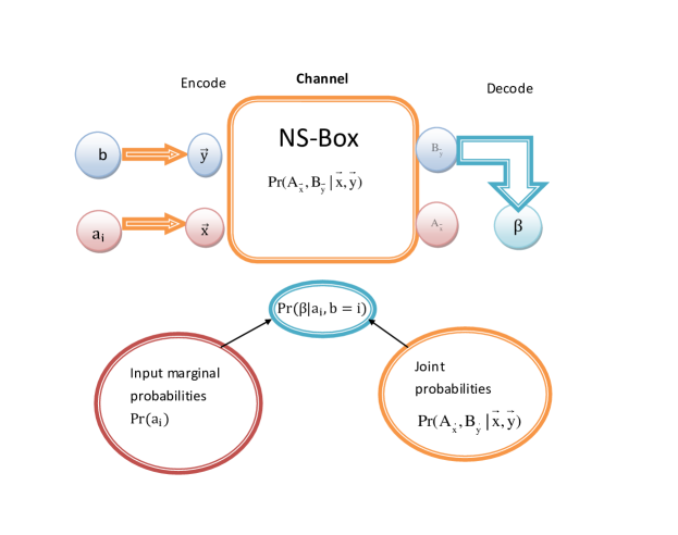
The above information gain $I$ is determined by three parts of the communication scheme: (1) the exact RAC protocol, (2) the communication channel and (3) the input marginal probabilities denoted by $\Pr(a_{i})$. This is shown in Fig 1. The purpose of RAC encoding is for Alice to encode her data $\vec{a}$ into $\vec{x}$ and Bob to do his $b$ into $\vec{y}$. The details will be given in section II.

The second part in our communication scheme is a given channel specified by the pre-shared correlation between Alice and Bob, the so-called no-signaling box (NS-box). The aforementioned encoded data $\vec{x}$ and $\vec{y}$ are the input of the NS-box which then yields the corresponding outputs $A_{\vec{x}}$ and $B_{\vec{y}}$, respectively. Bob will then combine $B_{\vec{y}}$ with the classical information sent from Alice to guess $\vec{a}$. Most importantly, the NS-box is characterized by the conditional joint probabilities $\Pr(A_{\vec{x}},B_{\vec{y}}|\vec{x},\vec{y})$, and should satisfy the following no-signaling condition no-signal

$$\sum_{B_{\vec{y}}}\Pr(A_{\vec{x}},B_{\vec{y}}|\vec{x},\vec{y})=\Pr(A_{\vec{x}}|\vec{x})\quad\mbox{and}\quad\sum_{A_{\vec{x}}}\Pr(A_{\vec{x}},B_{\vec{y}}|\vec{x},\vec{y})=\Pr(B_{\vec{y}}|\vec{y}),\qquad\forall\vec{x},\vec{y}.$$ (2)

This implies that superluminal signaling is impossible.

Now comes the third part in our communication scheme: the input marginal probabilities. They are usually assumed to be uniform and not treated as variables. However, when evaluating information gain $I$ in (1), we need the conditional probabilities $\Pr(\beta|a_{i},b=i)$, which are related to both the joint probabilities $\Pr(A_{\vec{x}},B_{\vec{y}}|\vec{x},\vec{y})$ of the NS-box and the input marginal probabilities $\Pr(a_{i})$. In this work, we will consider the more general communication schemes with variable and non-uniform $\Pr(a_{i})$ and evaluate the corresponding information gain.

Naively, one would like to find the information gain of our communication schemes by maximizing the information gain $I$ over $\Pr(a_{i})$ and $\Pr(A_{\vec{x}},B_{\vec{y}}|\vec{x},\vec{y})$. The joint probabilities of the NS-box $\Pr(A_{\vec{x}},B_{\vec{y}}|\vec{x},\vec{y})$ should be realized by the quantum correlations. However, we will show that this maximization problem is not a convex problem so that it cannot be solved by numerical recipes.

To by-pass this no-go situation, we choose two ways to proceed. The first way is to consider an alternative convex optimization problem, whose object function and the information gain $I$ are monotonically related under some special assumptions. It turns out that the alternative convex optimization problem is to find the maximal quantum violation of the Bell-type inequality. This can be thought as finding the generalized Tsirelson bound. We will call the corresponding inequality for the generalized Tsirelson bound the Tsirelson-type inequality, or simply the Tsirelson inequality. Correspondingly, the object function is the LHS of the Bell-type inequality, which we will call the Bell-type function, or simply Bell function.

For the binary 2-setting communication schemes, the Bell-type function is the famous CHSH function. However, for the general schemes one should try to find the appropriate Bell-type functions. In this paper, we generalize the construction method developed in Our to obtain such Bell-type functions. This method is based on the signal decay theorem proposed in Evans1 ; Evans2 . We further show that these Bell-type functions are monotonically related to $I$ for the communication schemes with unbiased (i.e., symmetric and isotropic) $\Pr(\beta|a_{i},b=i)$ and i.i.d. inputs $\{a_{i}\}$ with uniform $\Pr(a_{i})$. Therefore, for such schemes we can optimize the information gain $I$ by applying the semi-definite programing (SDP) method Acin ; Acinl to obtain the maximum of the Bell-type function for the quantum communication schemes, i.e., the Tsirelson bound.

On the other hand, if we would like to consider the more general communication schemes rather than the aforementioned ones so that the above monotonic relation between $I$ and the object function fails, then we will use the second way. This is just to maximize the information gain $I$ over $\Pr(a_{i})$ and $\Pr(A_{\vec{x}},B_{\vec{y}}|\vec{x},\vec{y})$ by brutal force numerically without relying on the convex optimization. As limited by the power of our computation facilities, we will only consider the binary 2-setting communication schemes. Our results show that the bound required by the information causality is not saturated by the scheme saturating the Tsirelson bound. Instead, it is saturated by the case saturating the CHSH inequality.

The paper is organized as follows. In the next section we will define our communication schemes in details and then derive the Bell-type functions for the schemes with unbiased $\Pr(\beta|a_{i},b=i)$ and i.i.d. inputs with uniform $\Pr(a_{i})$. In section III, we will show that maximizing the information gain $I$ over $\Pr(A_{\vec{x}},B_{\vec{y}}|\vec{x},\vec{y})$ and $\Pr(a_{i})$ is not a convex optimization problem. We also prove that the Bell-type functions and the information gain $I$ are monotonically related under some assumptions. In section IV, we briefly review the semidefinite programming (SDP) proposed in Acin ; Acinl , and then apply it to solve the convex optimization problem and find out the generalized Tsirelson bound. We use the result to evaluate the corresponding information gain $I$ and compare with the bound required by the information causality. In V, we will use the numerical brute-force method to maximize $I$ for general binary 2-setting schemes. Finally, we conclude our paper in section VI with some discussions. Besides, several technical detailed results are given in the Appendices.

II The generalized Bell-type functions from the signal decay theorem

In the Introduction, we have briefly described our communication scheme. Here we describe the details of the encoding/decoding in the RAC protocol: Alice encodes her data $\vec{a}$ as $\vec{x}:=(x_{1},\cdots,x_{k-1})$ with $x_{i}=a_{i}-a_{0}$, and Bob does his input $b$ as $\vec{y}:=(y_{1},\cdots,y_{k-1})$ with $y_{i}=\delta_{b,i}$ for $b\neq 0$ and $\vec{y}=0$ for $b=0$. The dit-string $\vec{x}$ and $\vec{y}$ are the inputs of the NS-box. The corresponding outputs of the NS-box are $A_{\vec{x}}$ and $B_{\vec{y}}$, respectively. More specifically, the dit sent by Alice is $\alpha=A_{\vec{x}}-a_{0}$, and the pre-shared correlation is defined by the conditional probabilities $\Pr(B_{\vec{y}}-A_{\vec{x}}=\vec{x}\cdot\vec{y}|\vec{x},\vec{y})$ between the inputs and outputs of the NS-box. Accordingly, Bob’s optimal guessing dit $\beta$ can be chosen as $B_{\vec{y}}-\alpha$. This is because $\beta=B_{\vec{y}}-A_{\vec{x}}+a_{0}=\vec{x}\cdot\vec{y}+a_{0}$ as long as $B_{\vec{y}}-A_{\vec{x}}=\vec{x}\cdot\vec{y}$ holds. In this case, Bob guesses $a_{b}$ perfectly. Take $d=3$ and $k=3$ as an example for illustration: Bob’s optimal guess bit is

$$\beta=\vec{x}\cdot\vec{y}+a_{0}=(a_{1}-a_{0},a_{2}-a_{0})\cdot(y_{0},y_{1})+a_{0}.$$ (3)

If Bob’s input $\vec{y}=(y_{0},y_{1})=(0,0)$, $\beta=a_{0}$; if $\vec{y}=(y_{0},y_{1})=(1,0)$, $\beta=a_{1}$; and if $\vec{y}=(y_{0},y_{1})=(0,1)$, $\beta=a_{2}$. Bob can guess $a_{b}$ perfectly.

Using the above RAC protocol, Alice and Bob have $d^{k-1}$ and $k$ measurement settings, respectively. Each of the measurement settings will give $d$ kinds of outputs. However, the noise of the NS-box affects the successful probability so that Bob can not always guess $a_{b}$ correctly. If the NS-box is a quantum mechanical one, then the conditional probabilities $\Pr(B_{\vec{y}}-A_{\vec{x}}=\vec{x}\cdot\vec{y}|\vec{x},\vec{y}])$ should be constrained by the Tsirelson-type inequalities, so are the joint probabilities $\Pr(A_{\vec{x}},B_{\vec{y}}|\vec{x},\vec{y})$. Then the question is how? For $d=2$ and $k=2$, the quantum constraint comes from the well-known Tsirelson inequality. That is, the maximal quantum violation of the CHSH inequality is $2\sqrt{2}$, i.e., $|C_{0,0}+C_{0,1}+C_{1,0}-C_{1,1}|\leq 2\sqrt{2}$. Note that, each term of CHSH function $C_{\vec{x},\vec{y}}$ can be expressed in terms of joint probabilities as $\Pr(00|\vec{x},\vec{y})-\Pr(01|\vec{x},\vec{y})-\Pr(10|\vec{x},\vec{y})+\Pr(11|\vec{x},\vec{y})$. Therefore, this is the constraint for $\Pr(A_{\vec{x}},B_{\vec{y}}|\vec{x},\vec{y})$ to be consistent with quantum mechanics.

However, there is no known Tsirelson-type inequalities for the cases with $d>2$. Despite that, in Our , we find a systematic way to construct $d=2$ and $k\geq 2$ Tsirelson-type inequalities by the signal decay theorem Evans1 ; Evans2 . We will generalize this method to $d>3$ case to yield suitable Bell-type functions. To proceed, we first recapitulate the derivation for $d=2$ cases.

Signal decay theory quantifies the loss of mutual information when processing the data through a noisy channel. Consider a cascade of two communication channels: $X\hookrightarrow Y\hookrightarrow Z$, then intuitively we have

$$I(X;Z)\leq I(X;Y).$$ (4)

Moreover, if the second channel is a binary symmetric one, i.e.,

$$\Pr(Z|Y)=\left(\begin{array}[]{cc}\frac{1}{2}(1+\xi)&\frac{1}{2}(1-\xi)\\ \frac{1}{2}(1-\xi)&\frac{1}{2}(1+\xi)\end{array}\right),$$

then the signal decay theorem says

$$\frac{I(X;Z)}{I(X;Y)}\leq\xi^{2}.$$ (5)

This theorem has been proven to yield a tight bound in Evans1 ; Evans2 . Note that the equality is held only when $\Pr(Y|X=0)$ and $\Pr(Y|X=1)$ are almost indistinguishable. For more detail, please see appendix A.

In Our , we set $X=a_{i}$, $Y=a_{0}+\vec{x}\cdot\vec{y}$ and $Z=\beta$. By construction, the bit $a_{i}$ is encoded as $a_{0}+\vec{x}\cdot\vec{y}$ such that $I(a_{i};a_{0}+\vec{x}\cdot\vec{y})=1$. Using the tight bound of (5), we can get

$$I(a_{i}\;;\beta|b=i)\leq\xi_{i}^{2}.$$ (6)

For our RAC protocol, the index of the $\xi_{i}$ is the vector $\vec{y}$. It is then easy to see that $\xi_{\vec{y}}$ is related to both the input marginal probabilities $\Pr(a_{i})$ and the joint probabilities of the NS-box by

$$\frac{1+\xi_{\vec{y}}}{2}=\sum_{\{\vec{x}\}}\Pr(\vec{x})\Pr\left(B_{\vec{y}}-A_{\vec{x}}=\vec{x}\cdot\vec{y}|\vec{x},\vec{y}\;\right).$$ (7)

Assuming that Alice’s database is i.i.d., we can then sum over all the mutual information between $\beta$ and $a_{i}$ to arrive

$$\sum_{i}I(a_{i}\;;\beta|b=i)\leq\sum_{i}\xi_{i}^{2}.$$ (8)

Though the object on the RHS is quadratic, we can linearize it by the Cauchy-Schwarz inequality, i.e., $|\sum_{i}\xi_{i}|\leq\sqrt{k\sum_{i}\xi_{i}^{2}}$. For $d=k=2$ case with uniform input marginal probabilities $\Pr(a_{i})$, it is easy to show that $\sum_{i}\xi_{i}\leq\sqrt{2}$ (or $\sum_{i}\xi_{i}^{2}\leq 1$) is nothing but the conventional Tsirelson inequality. Moreover, in Our we use the SDP algorithm in Wehner to generalize to $d=2$ and $k>2$ cases and show that the corresponding Tsirelson-type inequality is

$$\sum_{i}\xi_{i}\leq\sqrt{k}.$$ (9)

This is equivalent to say $\sum_{i}\xi^{2}\leq 1$. From the signal decay theorem (6) this implies that the maximal information gain in our RAC protocol with the pre-shared quantum resource is consistent with the information causality (1).

We now generalize the above construction to $d>2$ cases. First, we start with $d=3$ case by considering a cascade of two channels $X\hookrightarrow Y\hookrightarrow Z$ with the second one a 3-input, 3-output symmetric channel. Again, we want to find the upper bound of $\frac{I(X;Z)}{I(X;Y)}$. In the Appendix A we show that the ratio reaches an upper bound whenever three conditional probabilities $\Pr(Y|X=i)$ with $i=0,1,2$ are almost indistinguishable. Moreover, it can be also shown that the upper bound of the ratio is again given by (5) for the symmetric channel between $Y$ and $Z$ specified by

$$\Pr(Z|Y)=\left(\begin{array}[]{ccc}\frac{2\xi+1}{3}&\frac{1-\xi}{3}&\frac{1-\xi}{3}\\ \frac{1-\xi}{3}&\frac{2\xi+1}{3}&\frac{1-\xi}{3}\\ \frac{1-\xi}{3}&\frac{1-\xi}{3}&\frac{2\xi+1}{3}\end{array}\right).$$ (13)

One can generalize the above to the higher $d$ cases for the symmetric channel between $Y$ and $Z$ specified as follows: $\Pr(Z=i|Y=i)=\frac{(d-1)\xi+1}{d}$ and $\Pr(Z=s\neq i|Y=i)=\frac{1-\xi}{d}$ with $i\in\{0,1,...,d-1\}$. Again we will arrive (5). Based on the signal decay theorem with $X:=a_{i}$, $Y:=a_{0}+\vec{x}\cdot\vec{y}$ and $Z:=\beta$ and assuming that Alice’s input probabilities are i.i.d., we can sum over all the mutual information between each $a_{i}$ and $\beta$ and obtain

$$\sum_{i=0}^{k-1}I(\beta;a_{i}|b=i)\leq\sum_{i=0}^{k-1}\xi_{i}^{2}\log_{2}(d).$$ (14)

In our RAC protocol, the noise parameter $\xi_{\vec{y}}$ (or $\xi_{i}$) can be expressed as

$$\xi_{\vec{y}}=\frac{d\sum_{\vec{x}}\Pr(\vec{x})\Pr(B_{\vec{y}}-A_{\vec{x}}=\vec{x}\cdot\vec{y}|\vec{x},\vec{y})-1}{d-1}.$$ (15)

As for the $d=2$ case, we assume the upper bound of (14) is capped by the information causality to yield a quadratic constraint on the noise parameters. Again, using the Cauchy-Schwarz inequality to linearize the quadratic constraint, we find $\sum_{\vec{y}}\xi_{\vec{y}}\leq\sqrt{k}$. Especially, if the input marginal probabilities $\Pr(a_{i})$ are uniform, then this inequality yields a constraint on $\Pr(A_{\vec{x}},B_{\vec{y}}|\vec{x},\vec{y})$. Using (15), the LHS of this inequality can be thought as a Bell-type function, and our task is to check if the RHS matches with the Tsirelson bound or not.

Then, it is ready to ask the question: If the joint probabilities of a NS-box achieve the Tsirelson bound, does the same NS-box used in our RAC protocol also saturate the information causality bound? Next, we are going to address this question.

III Convexity and information gain

1 Feasibility for maximizing information gain by convex optimization

In order to test the information causality for more general communication schemes, we have to maximize the information gain $I$ over the conditional probabilities $\Pr(\beta|a_{i},b=i)$ determined by the joint probabilities $\Pr(A_{\vec{x}},B_{\vec{y}}|\vec{x},\vec{y})$ and $\Pr(a_{i})$. One way to achieve this task is to formulate the problem as a convex optimization programming, so that we may exploit some numerical recipes such as CVXOPT to carry out the task.

Minimizing a function with the equality or inequality constraints is called convex optimization. The object function could be linear or non-linear. For example, SDP is a kind of convex optimization with a linear object function. Regardless of linear or non-linear object functions, the minimization (maximization) problem requires them to be convex (concave). Thus, if we define the information gain $I$ as the object function for maximization in the context of information causality, we have to check if it is concave.

A concave function $f(x)$ ($f:\mathbb{R}^{n}\rightarrow\mathbb{R}$) should satisfy the following condition:

$$f(\lambda x_{1}+(1-\lambda)x_{2})\geq\lambda f(x_{1})+(1-\lambda)f(x_{2}),$$ (16)

where $x_{1}$ and $x_{2}$ are $n$-dimensional real vectors, and $0<\lambda<1$.

Mutual information between input $X$ and output $Z$ can be written as

$$I(X;Z)=H(Z)-H(Z|X)\\ =H(Z)-\sum_{i}\Pr(X=i)H(Z|X=i),$$ (17)

where $H(Z)=-\sum_{i}\Pr(Z=i)\log_{2}\Pr(Z=i)$ is the entropy function. We will study the convexity of $I(X;Z)$ by varying over the marginal probabilities $\Pr(X)$ and the channel probabilities $\Pr(Z|X)$.

The following theorem is mentioned in Tomas . If we fix the channel probabilities $\Pr(Z|X)$ in (17), then $I(X;Z)$ is a concave function with respect to $\Pr(X)$. This is the usual way in obtaining the channel capacity, i.e., maximizing information gain $I$ over the input marginal probabilities for a fixed channel.

However, in the context of information causality, the conditional probabilities $\Pr(\beta|a_{i},b=i)$ (or $\Pr(Z|X)$) are related to both the joint probabilities of the NS-box and the input marginal probabilities $\Pr(a_{i})$. This means that the above twos will be correlated if we fix $\Pr(\beta|a_{i},b=i)$. This cannot fit to our setup in which we aim to maximize the information gain $I$ by varying over the joint probabilities of NS-box and the input marginal probabilities $\Pr(a_{i})$. For example, in $d=2$ and $k=2$ case, $\Pr(\beta|a_{i},b=i)$ is given by

$$\Pr(\beta|a_{i},b=i)=\left(\begin{array}[]{cc}\alpha_{i}&1-\alpha_{i}\\ 1-\lambda_{i}&\lambda_{i}\end{array}\right).$$

where

$$\alpha_{0}:=\Pr(\beta=0|a_{0}=0,b=0) =\sum_{\ell=0}^{1}\Pr(B_{y}-A_{x}=0|x=\ell,y=0)\Pr(a_{1}=\ell),$$ (18)

$$\lambda_{0}:=\Pr(\beta=1|a_{0}=1,b=0) =\sum_{\ell=0}^{1}\Pr(B_{y}-A_{x}=0|x=\ell,y=0)\Pr(a_{1}=1-\ell),$$ (19)

$$\alpha_{1}:=\Pr(\beta=0|a_{1}=0,b=1) =\sum_{\ell=0}^{1}\Pr(B_{y}-A_{x}=\ell|x=\ell,y=1)\Pr(a_{0}=\ell),$$ (20)

$$\lambda_{1}:=\Pr(\beta=1|a_{1}=1,b=1) =\sum_{\ell=0}^{1}\Pr(B_{y}-A_{x}=\ell|x=\ell,y=1)\Pr(a_{0}=1-\ell).$$ (21)

From the above, we see that $\Pr(\beta|a_{i},b=i)$ cannot be fixed by varying over $\Pr(B_{y}-A_{x}|x,y)$ and $\Pr(a_{i})$ independently. Similarly, for higher $d$ and $k$ protocols, we will also have the constraints between the above three probabilities. Thus, maximizing the information gain for the information causality is different from the usual way of finding the channel capacity.

To achieve the goal of maximizing the information gain $I$ over the input marginal probabilities $\Pr(a_{i})$ and the joint probabilities $\Pr(B_{\vec{y}}-A_{\vec{x}}|\vec{x},\vec{y})$ which can be realized by quantum mechanics, we should check if it is a convex (or concave) optimization problem or not. If yes, then we can adopt the numerical recipe as CVXOPT to carry out the task. Otherwise, we can either impose more constraints for our problem or just do it by brutal force. It is known that Hassian one can check if maximizing function $f(y_{1},\cdots,y_{n})$ over $y_{i}$’s is a concave problem or not by examining its Hessian matrix

$$H(f)=\left(\begin{array}[]{cccc}\frac{\partial^{2}f}{\partial y_{1}^{2}}&\frac{\partial^{2}f}{\partial y_{1}y_{2}}&\cdots&\frac{\partial^{2}f}{\partial y_{1}y_{n}}\\ \frac{\partial^{2}f}{\partial y_{2}y_{1}}&\frac{\partial^{2}f}{\partial y_{2}^{2}}&\cdots&\frac{\partial^{2}f}{\partial y_{2}y_{n}}\\ \vdots&\vdots&\ddots&\vdots\\ \frac{\partial^{2}f}{\partial y_{n}y_{1}}&\frac{\partial^{2}f}{\partial y_{n}y_{2}}&\cdots&\frac{\partial^{2}f}{\partial y_{n}^{2}}\\ \end{array}\right).$$ (26)

For the maximization to be a concave problem, the Hessian matrix should be negative semidefinite. That is, all the odd order principal minors of $H(f)$ should be negative and all the even order ones should be positive. Note that each first-order principal minor of $H(f)$ is just the second derivative of $f$, i.e. ${\partial^{2}f\over\partial y_{i}^{2}}$. So, the problem cannot be concave if ${\partial^{2}f\over\partial y_{i}^{2}}>0$ for some $i$.

With the above criterion, we can now show that the problem of maximizing $I$ over $\Pr(B_{\vec{y}}-A_{\vec{x}}|\vec{x},\vec{y})$ and $\Pr(a_{i})$ cannot be a concave problem. To do this, we rewrite the information gain $I$ defined in (1) as following:

$$I=\sum_{i=0}^{k-1}\sum_{n=0}^{d-1}\sum_{j=0}^{d-1}\Pr(\beta=n,a_{i}=j|b=i)\log_{2}\frac{\Pr(\beta=n,a_{i}=j|b=i)}{\Pr(\beta=n|b=i)\Pr(a_{i}=j)}.$$ (27)

Furthermore, one can express the above in terms of $\Pr(B_{\vec{y}}-A_{\vec{x}}|\vec{x},\vec{y})$ and $\Pr(a_{i})$ by the following relations

$$\Pr(\beta=n,a_{i}=j|b=i) =\sum_{\{a_{k\neq i}\}}\Pr(B_{\vec{y}}-A_{\vec{x}}=n-a_{0}|\vec{x},\vec{y})\Pr(a_{i}=j)\;\Pi_{k\neq i}\Pr(a_{k}),$$ (28)

$$\Pr(\beta=n|b=i) =\sum_{j=0}^{d-1}\Pr(\beta=n,a_{i}=j|b=i),$$ (29)

where $\vec{x}$ and $\vec{y}$ in the above are given by the RAC encoding, i.e., $\vec{x}:=(x_{1},\cdots,x_{k-1})$ with $x_{i}=a_{i}-a_{0}$ and $\vec{y}:=(y_{1},\cdots,y_{k-1})$ with $y_{i}=\delta_{b,i}$ for $b\neq 0$ and $\vec{y}=0$ for $b=0$.

Moreover, both $\Pr(B_{\vec{y}}-A_{\vec{x}}|\vec{x},\vec{y})$ and $\Pr(a_{i})$ are subjected to the normalization conditions of total probability. Thus we need to solve these conditions such that the information gain $I$ is expressed as the function of independent probabilities. After that, we can evaluate the corresponding Hessian matrix to examine if the maximization of $I$ over these probabilities is a concave problem or not.

For illustration, we first consider the $d=2$ and $k=2$ case. By using the relations (28) and the normalization conditions of total probability to implement the chain-rule while taking derivative, we arrive

$$\frac{\ln 2\cdot\partial^{2}I}{\partial(\Pr(B_{y}-A_{x}=0|x=0,y=0))^{2}}=$$

$$-(\frac{1}{\Pr(\beta=0|b=0)}+\frac{1}{\Pr(\beta=1|b=0)})(\Pr(a_{0}=0)\Pr(a_{1}=0)-\Pr(a_{0}=1)\Pr(a_{1}=1))^{2}$$

$$+(\Pr(a_{0}=0)\Pr(a_{1}=0))^{2}(\frac{1}{\Pr(\beta=0,a_{0}=0|b=0)}+\frac{1}{\Pr(\beta=1,a_{0}=0|b=0)})$$

$$+(\Pr(a_{0}=1)\Pr(a_{1}=1))^{2}(\frac{1}{\Pr(\beta=0,a_{0}=1|b=0)}+\frac{1}{\Pr(\beta=1,a_{0}=1|b=0)}).$$ (30)

Obviously, (1) cannot always be negative. This can be seen easily if we set $\Pr(a_{0})=1-\Pr(a_{1})$ so that the first term on the RHS of (1) is zero. Then, the remaining terms are non-negative definiteness. This then indicates that maximizing $I$ over the joint probabilities is not a concave problem.

The check for the higher $d$ and $k$ cases can be done similarly, and the details can be found in the Appendix B. Again, we can set all the $\Pr(a_{i})$ to be uniform so that we have

$$\frac{d^{2k}\ln 2\cdot\partial^{2}I}{\partial(\Pr(B_{\vec{y}}-A_{\vec{x}}=0|\vec{x}=\vec{0},\vec{y}=\vec{0}))^{2}}=$$

$$\sum_{n=0}^{d-1}(\frac{1}{\Pr(a_{0}=n,\beta=n|b=0)}+\frac{1}{\Pr(a_{0}=n,\beta=n+1-d|b=0)})>0.$$ (31)

2 Convex optimization for the unbiased conditional probabilities with i.i.d. and uniform input marginal probabilities

Recall that we would like to check if the boundaries of the information causality and the generalized Tsirelson bound agree or not. To achieve this, we may maximize the information gain $I$ with the joint probabilities $\Pr(A_{\vec{x}},B_{\vec{y}}|\vec{x},\vec{y})$ realized by quantum mechanics. Or, we may find the generalized Tsirelson bound and then evaluate the corresponding information gain $I$ which can be compared with the bound of information causality. These two tasks are not equivalent but complementary. However, unlike the first task, the second task will be concave problem as known in Wehner ; Acinl . The only question in this case is if the corresponding information gain $I$ is monotonically related to the Bell-type functions or not. If yes, then finding the generalized Tsirelson bound is equivalent to maximizing the information gain $I$ in our communication schemes. The answer is partially yes as we will show this monotonic relation holds only for the unbiased conditional probabilities $\Pr(\beta|a_{i},b=i)$ with i.i.d. and uniform input marginal probabilities $\Pr(a_{i})$.

The unbiased conditional probabilities $\Pr(\beta|a_{i},b=i)$ are symmetric and isotropic. This is defined as follows. One can construct a matrix $CP$ with the matrix elements $CP_{j+1,k+1}=\Pr(\beta=k|a_{i}=j,b=i)$ with $j,k\in\{0,1,...,d-1\}$. If all the rows of matrix $CP$ are permutation for each other and all columns are also permutation for each other, the conditional probabilities $\Pr(\beta|a_{i},b=i)$ are symmetric. Moreover, if the symmetric conditional probabilities $\Pr(\beta|a_{i},b=i)$ for different $i$ are the same, the conditional probabilities $\Pr(\beta|a_{i},b=i)$ are isotropic.

Assuming Alice’s input is i.i.d., we have Shannon entropy $H(\beta|b=i)=\log_{2}d$. As $\Pr(\beta|a_{i},b=i)$ are unbiased, they are symmetric so that $\Pr(\beta=t|a_{i}=j,b=i)=\frac{(d-1)\xi_{i}+1}{d}$ for $t=j$, and $\Pr(\beta=t|a_{i}=j,b=i)=\frac{1-\xi_{i}}{d}$ for $t\neq j$. Thus, the information gain $I$ becomes

$$I=k\log_{2}d+\sum_{i=0}^{k-1}[\frac{(d-1)\xi_{i}+1}{d}\log_{2}(\frac{(d-1)\xi_{i}+1}{d})+(1-\frac{(d-1)\xi_{i}}{d})\log_{2}(\frac{1-\xi_{i}}{d})].$$ (32)

Moreover, $\Pr(\beta|a_{i},b=i)$ are also isotropic, therefore $\xi_{i}=\xi$ $\forall i$. For such a case the information gain $I$ can be further simplified to

$$I=k[\log_{2}d+\frac{(d-1)\xi+1}{d}\log_{2}(\frac{(d-1)\xi+1}{d})+(1-\frac{(d-1)\xi}{d})\log_{2}(\frac{1-\xi}{d})].$$ (33)

The value of $\xi$ is in the interval $[0,1]$. As $\xi$ is the noise parameter of the channel with input $a_{i}$ and output $\beta$, then $\xi=0$ for the completely random channel and $\xi=1$ for the noiseless one, i.e., $\Pr(\beta=t|a_{i}=j,b=i)=\frac{1}{d}$ for $\xi=0$ and $\Pr(\beta=t|a_{i}=t,b=i)=1$ for $\xi=1$.

We can show that the information gain $I$ is monotonically increasing with the Bell-type functions parameterized by the noise parameter $\xi$. To see this, we calculate the first and second derivative of $I$ with respect to $\xi$ and obtain

$$\frac{dI}{d\xi}=\frac{d-1}{d}\log\frac{(d-1)\xi+1}{1-\xi},$$

$$\frac{d^{2}I}{d\xi^{2}}=\frac{d-1}{d}(\frac{d-1}{(d-1)\xi+1}+\frac{1}{1-\xi}).$$

From the above, we see that $\frac{dI}{d\xi}$ is always positive for $\xi\in[0,1]$. Moreover, it is easy to see that $I$ is minimal at $\xi=0$ since $\frac{d^{2}I}{d\xi^{2}}=d-1>0$. Thus, if the RAC protocol has i.i.d. and uniform input marginal probabilities, the information gain $I$ is a monotonically increasing function of $\xi$ for the the unbiased conditional probabilities $\Pr(\beta|a_{i},b=i)$.

IV Finding the quantum violation of the Bell-type inequalities from the hierarchical semi-definite programming

We now will prepare for numerically evaluating the maximum of the Bell-type function

$$\sum_{\vec{y}}\xi_{\vec{y}}\qquad\mbox{with $\xi_{\vec{y}}$ given in (\ref{xi}) \; and \; $\Pr(a_{i})={1\over d},\;\forall a_{i},i$.}$$ (34)

It is monotonic increasing with information gain $I$ under some assumptions. In order to ensure that the maximum of (34) can be obtained by quantum resource, we have to use the same method as in Acin ; Acinl . In Acin ; Acinl , they checked if a given set of probabilities can be reproduced from quantum mechanics or not. This task can be formulated as solving a hierarchy of semidefinite programming (SDP).

1 Projection operators with quantum behaviors

We will now briefly review the basic ideas in Acin ; Acinl and then explain how to use it for our program. In Acin ; Acinl they use the projection operators for the following measurement scenario. Two distant partite Alice and Bob share a NS-box. Alice and Bob input $X$ and $Y$ to the NS-box, respectively, and obtain the corresponding outputs $a\in A$ and $b\in B$. Here $A$ and $B$ are used to denote the set of all possible Alice’s and Bob’s measurement outcomes, respectively. We use $X(a)$ and $Y(b)$ to denote the corresponding inputs. These outcomes can be associated with some sets of projection operators $\{E_{a}:a\in A\}$ and $\{E_{b}:b\in B\}$. The joint probabilities of the NS-box can then be determined by the quantum state $\rho$ of the NS-box and the projection operators as following:

$$\Pr(a,b)=\mbox{Tr}(E_{a}E_{b}\rho).$$ (35)

Note that $\Pr(a,b)$ is the abbreviation of $\Pr(A_{\vec{x}},B_{\vec{y}}|\vec{x},\vec{y})=\mbox{Tr}(E_{A_{\vec{x}}}E_{B_{\vec{y}}}\rho)$ defined in the previous sections.

If $E_{a}$ and $E_{b}$ are the genuine quantum operators, then they shall satisfy (i) hermiticity: $E^{{\dagger}}_{a}=E_{a}$ and $E^{{\dagger}}_{b}=E_{b}$; (ii) orthogonality: $E_{a}E_{a^{\prime}}=\delta_{aa^{\prime}}$ if $X(a)=X(a^{\prime})$ and $E_{b}E_{b^{\prime}}=\delta_{b,b^{\prime}}$ if $Y(b)=Y(b^{\prime})$; (iii) completeness: $\Sigma_{a\in X}E_{a}=\mathbb{I}$ and $\Sigma_{b\in Y}E_{b}=\mathbb{I}$; and (iv) commutativity: $[E_{a},E_{b}]=0$.

In our measurement scenario, the distant partite Alice and Bob perform local measurements so that property (iv) holds. On the other hand, the property (iii) implies no-signaling as it leads to (2) via (35). Furthermore, this property also implies that there is redundancy in specifying Alice’s operators $E_{a}$’s with the same input since one of them can be expressed by the others. Thus, we can eliminate one of the outcomes per setting and denote the corresponding sets of the remaining outcomes for the input $X$ by $\tilde{A}_{X}$ (or $\tilde{B}_{Y}$ for Bob’s outcomes with input $Y$). The collection of such measurement outcomes $\bigoplus_{X}\tilde{A}_{X}$ is denoted as $\tilde{A}$. Similarly, we denote the collection of Bob’s independent outcomes as $\tilde{B}$.

Using the reduced set of projection operators $\{E_{a}:a\in\tilde{A}\}$ and $\{E_{b}:b\in\tilde{B}\}$, we can construct a set of operators $\emph{O}=\{O_{1},O_{2},...,O_{i},...\}$. Here $O_{i}$ is some linear function of products of operators in $\{\mathbb{I}\cup\{E_{a}:a\in\tilde{A}\}\cup\{E_{b}:b\in\tilde{B}\}\}$. The set O is characterized by a matrix $\Gamma$ given by

$$\Gamma_{ij}=\mbox{Tr}(O^{{\dagger}}_{i}O_{j}\rho).$$ (36)

By construction, $\Gamma$ is non-negative definite, i.e.,

$$\Gamma\succeq 0.$$ (37)

This can be easily proved as follows. For any vector $v\in\mathbb{C}^{n}$ (assuming $\Gamma$ is a $n$ by $n$ matrix), one can have

$$v^{{\dagger}}\Gamma v=\Sigma_{s,t}v^{*}_{s}\mbox{Tr}(O^{{\dagger}}_{s}O_{t}\rho)v_{t}=\mbox{Tr}(V^{{\dagger}}V\rho)\geq 0.$$ (38)

Recall that our goal is to judge if a given set of joint probabilities such as (35) can be reproduced by quantum mechanics or not. In this prescription, the joint probabilities are then encoded in the matrix $\Gamma$ satisfying the quantum constraints (35) and (37). However, $\Gamma$ contains more information than just joint probabilities (35). For examples, the terms appearing in the elements of $\Gamma$ such as $\mbox{Tr}(E_{a}E_{a^{\prime}}\rho),\mbox{Tr}(E_{b}E_{b^{\prime}}\rho)$ for $X(a)\neq X(a^{\prime})$ and $Y(b)\neq Y(b^{\prime})$ can not be expressed in terms of the joint probabilities of the NS-box. This is because these measurements are performed on the same partite (either Alice or Bob) and are not commutative. Therefore, to relate the joint probabilities of the NS-box to the matrix $\Gamma$, we need to find the proper combinations of $\Gamma_{ij}$ so that the final object can be expressed in terms of only the joint probabilities. Therefore, given the joint probabilities, there shall exist some matrix functions $F_{q}$’s such that the matrix $\Gamma$ is constrained as follows:

$$\Sigma_{s,t}(F_{q})_{s,t}\Gamma_{s,t}=g_{q}$$ (39)

where $g_{q}$’s are the linear functions of joint probabilities $\Pr(a,b)$’s.

We then call the matrix $\Gamma$ a certificate if it satisfies (37) and (39) for a given set of joint probabilities of NS-box. The existence of the certificate will then be examined numerically by SDP. If the certificate does not exist, the joint probabilities cannot be reproduced by quantum mechanics.

Examples on how to construct $F_{q}$ and $g_{q}$ for some specific NS-box protocols can be found in Acin ; Acinl . For illustration, here we will explicitly demonstrate the case not considered in Acin ; Acinl , that is the $k=2$, $d=3$ RAC protocol. We will use the notation which we defined in the previous sections. We start by defining the set of operators $\mathcal{E}=\{\mathcal{E}_{i}\}:=\mathbb{I}\cup\{E_{A_{x}}:A_{x}\in\{0,1\},x\in\{0,1,2\}\}\cup\{E_{B_{y}}:B_{y}\in\{0,1\},y\in\{0,1\}\}$ with the operator label $i\in\{0,1,2,...,m_{a},....,m_{a}+m_{b}\}$. The operator $\mathcal{E}_{i=0}$ is the identity operator $\mathbb{I}$, and $\mathcal{E}_{1<i\leq m_{a}}\in E_{A_{x}}$, $\mathcal{E}_{m_{a}<i\leq m_{a}+m_{b}}\in E_{B_{y}}$.

The associated quantum constraints can be understood as the relations between joint probabilities $\Pr(a,b)$ and $\mbox{Tr}(\mathcal{E}^{\dagger}_{a}\mathcal{E}_{b}\rho)$ (or marginal probabilities $\Pr(a)$ and $\mbox{Tr}(\mathbb{I}\mathcal{E}_{a}\rho)$). That is,

$$\mbox{Tr}(\rho)=1,\qquad\mbox{Tr}(\mathbb{I}E_{A_{x}}\rho)=\Pr(A_{x}|x),\qquad\mbox{Tr}(\mathbb{I}E_{B_{y}}\rho)=\Pr(B_{y}|y),$$

$$\mbox{Tr}(E_{A_{x}}E_{A_{x}^{\prime}}\rho)=\delta_{A_{x},A_{x}^{\prime}}\Pr(A_{x}|x),\mbox{Tr}(E_{B_{y}}E_{B_{y}^{\prime}}\rho)=\delta_{B_{y},B_{y}^{\prime}}\Pr(B_{y}|y),$$

$$\mbox{Tr}(E_{A_{x}}E_{B_{y}}\rho)=\Pr(A_{x},B_{y}|x,y).$$ (40)

Note that these equations also hold when permuting the operators, i.e., $\mbox{Tr}(E_{A_{x}}E_{B_{y}}\rho)=\mbox{Tr}(E_{B_{y}}E_{A_{x}}\rho)$.

Moreover, we can make the matrix $\Gamma$ to be real and symmetric by redefining it as $\Gamma=(\Gamma^{*}+\Gamma)/2$. Thus, in the following we will only display the upper triangular part of $\Gamma$. We then use the quantum constraints (1) to construct $F_{q}$ and $g_{q}$ by comparing them with (39). We then see that every constraint in (1) yields a matrix function $F_{q}$ which has only one non-zero element, and also yields a function $g_{q}$ which is either zero or contains only a single term of a marginal or joint probabilities. These constraints can be further divided into four subsets labeled by $q=(q_{1},q_{2},q_{3},q_{4})$ as follows:

1. The labels $q_{1},q_{2}\in\{0,1,...,m_{a}+m_{b}\}$ are used to specify the marginal probabilities $\mbox{Tr}(\mathbb{I}\mathcal{E}_{q_{1}}\rho)$ and $\mbox{Tr}(\mathcal{E}^{\dagger}_{q_{2}}\mathcal{E}_{q_{2}}\rho)$. The corresponding matrix functions $F_{q}$ are given by $(F_{q_{1}})_{s,t}=\delta_{s,1}\delta_{t,q_{1}+1}$ and $(F_{q_{2}})_{s,t}=\delta_{s,q_{2}+1}\delta_{t,q_{2}+1}$, and the $g_{q_{1}}$ and $g_{q_{2}}$ are the corresponding marginal probabilities.

2. The label $q_{3}\in\{1,...,d^{k-1}+k\}$ is used to specify the probabilities associated with the orthogonal operator pairs, $\mbox{Tr}(\mathcal{E}_{2q_{3}-1}\mathcal{E}_{2q_{3}}\rho)$. The matrix element $(F_{q_{3}})_{s,t}=\delta_{s,2q_{3}}\delta_{t,2q_{3}+1}$, and $g_{q_{3}}=0$.

3. The label $q_{4}\in\{1,...,m_{a}m_{b}\}=4(2x+A_{x})+(2y+B_{y}+1)$ is used to specify the joint probabilities of the NS-box. The corresponding $F_{q}$ and $g_{q}$ are given by $(F_{q_{4}})_{s,t}=\delta_{s,2x+A_{x}+2}\delta_{t,m_{a}+2y+B_{y}+2}$, and $g_{q_{4}}=\Pr(A_{x},B_{y}|x,y)$.

Considering the above set of quantum constraint, we can define the associated $\Gamma$ matrix

$$\Gamma=\scriptsize\left(\begin{array}[]{ccccccccccc}1&\Pr(0|0)_{A}&\Pr(1|0)_{A}&\Pr(0|1)_{A}&\Pr(1|1)_{A}&\Pr(0|2)_{A}&\Pr(1|2)_{A}&\Pr(0|0)_{B}&\Pr(1|0)_{B}&\Pr(0|1)_{B}&\Pr(1|1)_{B}\\ &\Pr(0|0)_{A}&0&\chi_{0}&\chi_{1}&\chi_{2}&\chi_{3}&\Pr(00|00)&\Pr(01|00)&\Pr(00|01)&\Pr(01|01)\\ &&\Pr(1|0)_{A}&\chi_{4}&\chi_{5}&\chi_{6}&\chi_{7}&\Pr(10|00)&\Pr(11|00)&\Pr(10|01)&\Pr(11|01)\\ &&&\Pr(0|1)_{A}&0&\chi_{8}&\chi_{9}&\Pr(00|10)&\Pr(01|10)&\Pr(00|11)&\Pr(01|11)\\ &&&&\Pr(1|1)_{A}&\chi_{10}&\chi_{11}&\Pr(10|10)&\Pr(11|10)&\Pr(10|11)&\Pr(11|11)\\ &&&&&\Pr(0|2)_{A}&0&\Pr(00|20)&\Pr(01|20)&\Pr(00|21)&\Pr(01|21)\\ &&&&&&\Pr(1|2)_{A}&\Pr(10|20)&\Pr(11|20)&\Pr(10|21)&\Pr(11|21)\\ &&&&&&&\Pr(0|0)_{B}&0&\chi_{12}&\chi_{13}\\ &&&&&&&&\Pr(1|0)_{B}&\chi_{14}&\chi_{15}\\ &&&&&&&&&\Pr(0|1)_{B}&0\\ &&&&&&&&&0&\Pr(1|1)_{B}\\ \end{array}\right),$$ (52)

where $\Pr(A_{x}|x)_{A}$’s and $\Pr(B_{y}|y)_{B}$’s are the marginal probabilities for Alice and Bob, respectively, and $\Pr(A_{x},B_{y}|x,y)$’s are the joint probabilities of the NS-box. The elements $\chi_{i}$’s in the above cannot be defined by the given marginal and joint probabilities because they correspond to the probabilities of different measurement settings for only one party. Thus, they cannot appear in the constraints (39) but are still constrained by the non-negative definiteness of $\Gamma$.

Testing the existence of the certificate— The task of testing the existence of the certificate can be formulated as a SDP by defining the standard primal and the associated dual problems. The details can be found in Appendix C. The primal problem of SDP is subjected to certain conditions associated with a positive semi-definite matrix, which can be either linear equalities or inequalities. Each primal problem has an equivalent dual problem. Therefore, when the optimal value of the primal problem is the same as the optimal value of the dual problem, the feasible solution of the problem is obtained.

For our case the primal problem of SDP is as follows:

$$maximize\qquad \lambda$$ (53a)

$$subject\quad to\qquad \mbox{Tr}(F_{q}^{T}\Gamma)=g_{q},\qquad q=1,...,m,$$ (53b)

$$\Gamma-\lambda\mathbb{I}\succeq 0.$$ (53c)

Obviously, if the maximal value $\lambda\geq 0$ is obtained, the non-negative definiteness of $\Gamma$ is guaranteed under the quantum constraints (37).

On the other hand, the associated dual problem is given by

$$maximize\qquad \sum_{q}y_{q}g_{q},$$ (54a)

$$subject\quad to\qquad \sum_{q}y_{q}F_{q}^{T}\succeq 0,$$ (54b)

$$\sum_{q}y_{q}\mbox{Tr}(F_{q}^{T})=1.$$ (54c)

Note that the quantity $\sum_{q}y_{q}g_{q}$ is the Bell-type function since $g_{q}$’s are mainly the two-point correlation function. Therefore, maximizing this quantity is equivalent to finding the generalized Tsireslon bound. That is, if the solution of this SDP is feasible, then the associated certificate exists and there yields the generalized Tsireslon bound.

2 Hierarchy of the semi-definite programming

Different operator sets O’s yield different quantum constrains (35) and (37). There seems no guideline in choosing the set O and examining the existence of the corresponding certificate. However, it is easy to see that the certificates associated with different operator sets are equivalent. This can be seen as follows. Let us assume O and $\emph{O}^{\prime}$ are two linearly equivalent set of operators such that $O_{i}\in\emph{O}$ can be expressed by a linear combination of the elements in $\emph{O}^{\prime}$, i.e., $O_{i}=\sum_{j}C_{i,j}O_{j}^{{}^{\prime}}$. If there exists a matrix $\Gamma^{\prime}$ satisfying (37) and(39) for the corresponding operator set $\emph{O}^{\prime}$, then there will exist another matrix $\Gamma$ whose elements $\Gamma_{s,t}=\sum_{q,l}C_{q,s}^{*}\Gamma_{q,l}^{{}^{\prime}}C_{l,t}$ are also satisfying (37) and (39) for the set O. Therefore, we only need to stick to one set of operators in this linear equivalence class when examining the existence of the corresponding certificate.

Besides, a systematic way of constructing O is proposed in Acin ; Acinl so that the task of finding the certificate can be formulated as solving a hierarchy of SDP. This is constructed as follows. The length of the operator $O_{i}$, denoted by $|\emph{O}_{i}|$, is defined as the minimal number of projectors used to construct it. We can then divide the set O into different subsets labeled by the maximal length of the operators in the corresponding subset. Thus, we decompose the operator set O into a sequence of hierarchical operator sets denoted by $S_{n}$ where $n$ is the maximal length of the operators in $S_{n}$. That is,

$$S_{0}=\{{\mathbb{I}}\}$$

$$S_{1}=\{S_{0}\}\cup\{E_{a}:a\in\tilde{A}\}\cup\{E_{b}:b\in\tilde{B}\}$$

$$S_{2}=\{S_{0}\}\cup\{S_{1}\}\cup\{E_{a}E_{a^{\prime}}:a,a^{\prime}\in\tilde{A}\}\cup\{E_{b}E_{b^{\prime}}:b,b^{\prime}\in\tilde{B}\}\cup$$

$$\{E_{a}E_{b}:a\in\tilde{A},b\in\tilde{B}\}$$

$$...$$ (55)

Furthermore, to save the computer memory space used in the numerical SDP algorithm, in the above sequence we can add an intermediate set between $S_{n}$ and $S_{n+1}$, which is given by $S_{n+AB}:=\{S_{n}\}\cup\{S\in S_{n+1}|S=E_{a}E_{b}S^{\prime}:a\in\tilde{A},b\in\tilde{B}\}$. For example, when $n=1$ we have $S_{1+AB}=\{S_{1}\}\cup\{E_{a}E_{b}:a\in\tilde{A},b\in\tilde{B}\}$ such that $S_{1}\subseteq S_{1+AB}\subseteq S_{2}$. Note that $S_{1+AB}$ doesn’t have the product of the marginal projection operators in the form of $\{E_{a}E_{a^{\prime}}:a,a^{\prime}\in\tilde{A}\}$ and $\{E_{b}E_{b^{\prime}}:b,b^{\prime}\in\tilde{B}\}$. It is clear that $S_{1+AB}\subseteq S_{2}$. All the operators in O can be expressed in terms of the linear combination of the operators in $S_{n}$ for large enough $n$.

Figure 2: The geometric interpretation of collection $Q_{n}$

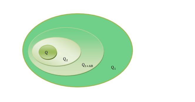
Since we know $S_{n}\subseteq S_{n+AB}\subseteq S_{n+1}$, the associated constraints produced by $S_{n+1}$ is stronger than $S_{n+AB}$ and $S_{n}$. We can start the task from $S_{1}$ then $S_{1+AB}$, $S_{2}$ and so on. Let the certificate matrix associated with the set $S_{n}$ be denoted as $\Gamma^{(n)}$. Finding the certificate associated with this sequence can be formulated as a hierarchical SDP. Once the given joint probabilities satisfy the quantum constraints (37) so that the associated certificate $\Gamma^{(n)}$ exists, we then denote the collection of these joint probabilities as $Q_{n}$. Since we know that the associated constraints are stronger than the previous steps of the hierarchical sequence, the collection $Q_{n}$ will become smaller for the higher $n$. That is, the non-quantum correlations will definitely fail the test at some step in the hierarchical SDP. The geometrical interpretation of the above fact is depicted in Fig 2.

It was shown in Acin ; Acinl that the probability is ensured to be quantum only when the certificate associated with $S_{n\rightarrow\infty}$ exists, i.e., for the joint probabilities in the collection $Q$ of Fig 2. In this sense, it seems that we have to check infinite steps. To cure this, a stopping criterion is proposed in Acin ; Acinl to terminate the check process at some step of the hierarchical SDP. This can ensure that the given joint probabilities are quantum at finite $n$ if the stopping criterion is satisfied.

The stopping criterion is satisfied when the rank of sub-matrix of $\Gamma^{(n)}$ is equal to the rank of $\Gamma^{(n)}$, i.e.,

$$rank(\Gamma_{X,Y}^{(n)})=rank(\Gamma^{(n)}).$$ (56)

The element of $\Gamma_{X,Y}^{(n)}$ is constructed by the operators in the set $S_{X,Y}:=\{S_{n-1}\}\bigcup\{S=E_{a}E_{b}S^{\prime}:a\in\tilde{A}_{X},b\in\tilde{B}_{Y},|S|\leq n\}$.

The above stopping criterion is for integer $n$. However, it was also generalized in Acinl for the intermediate certificate $\Gamma^{(n+AB)}$: the stopping criterion is satisfied if the following equation is satisfied for all the measurement settings $X$ and $Y$,

$$rank(\Gamma^{(n+XY)})=rank(\Gamma^{(n+AB)}),$$ (57)

so that the certificate $\Gamma^{(n+AB)}$ has a rank loop. Here $\Gamma^{(n+XY)}$ is the certificate associated with $S_{n+XY}:=\{S_{n}\}\cup\{S\in S_{n+1}|S=E_{a}E_{b}S^{\prime}:a\in\tilde{A}_{X},b\in\tilde{B}_{Y}\}$.

Now we are ready to implement the above criterion to numerically examine the quantum behaviors of the given joint probabilities for our RAC protocols with higher $k$ and $d$.

3 The quantum violation of the Bell-type inequalities and the corresponding information gain in the hierarchical semi-definite programming

Any Bell-type function including (34) can be written as the linear combination of joint probabilities, then the hierarchical SDP can be used to approach the quantum bound of the Bell-type functions (the generalized Tsirelson bound). Recall that the value of the Bell-type functions and the information gain $I$ are monotonically related for the unbiased conditional probabilities $\Pr(\beta|a_{i},b=i)$ with i.i.d. and uniform input marginal probabilities $\Pr(a_{i})$. After obtaining the maximum of the Bell-type functions at each step of the aforementioned hierarchical SDP, we can calculate the corresponding information gain $I$ and compare with the information causality. Since the quantum constraint is stronger in the hierarchical SDP and the collection of $Q_{n}$ will become smaller while $n$ is increasing. We then know that the bound of the Bell-type functions and the associated information gain $I$ will become tighter for larger $n$ and it will converge to the quantum bound for large enough $n$. Once the bound of information gain $I$ at some step of hierarchy doesn’t saturate the information causality, we can then infer that the quantum bound of information gain will not saturate the information causality, too.

First, let us discuss how to find the generalized Tsirelson bound of the Bell-type functions. As discussed before, the problem of finding the generalized Tsirelson bound can be reformulated as a SDP. The primal problem of this SDP is defined as

$$maximize\qquad \mbox{Tr}(C^{T}\Gamma^{(n)})$$ (58a)

$$subject\quad to\qquad \mbox{Tr}(F_{q}^{T}\Gamma^{(n)})=g_{q}(p),\quad q=1,\cdots,m;$$ (58b)

$$\Gamma^{(n)}\succeq 0.$$ (58c)

$$\mbox{Tr}(H_{w}^{T}\Gamma^{(1)})\geq 0,\quad w=1,\cdots,s;$$ (58d)

The matrix $C$ is given to make $\mbox{Tr}(C^{T}\Gamma^{(n)})$ the Bell-type functions which we would like to maximize. Eq. (58b) and (58c) are the quantum constraints discussed in the previous subsections so that the quantum behaviors are ensured during the SDP procedure. Moreover, with proper choice of the matrix $H_{w}$ , the condition (58d) is introduced to ensure the non-negativity of the joint probabilities which are the off-diagonal elements of $\Gamma^{(1)}$.

In the following we define the matrix $C$ for our case. Eq. (34), which can be expressed as the linear combination of the joint probabilities, i.e., $\sum_{\vec{x},\vec{y}}\Pr(B_{\vec{y}}-A_{\vec{x}}=\vec{x}\cdot\vec{y}|\vec{x},\vec{y})$, is the object for our SDP (58). Since we only consider $d-1$ marginal probabilities per measurement setting, we should further rewrite our object according to the completeness conditions, i.e., $\Sigma_{a\in X}E_{a}=\mathbb{I}$ and $\Sigma_{b\in Y}E_{b}=\mathbb{I}$. After rewriting, we can write down the matrix $C$ in (58). We take $d=3$, $k=2$ RACs protocol for example. For $\Gamma^{(1)}$,

$$C=\frac{1}{2}\left(\begin{array}[]{ccccccccccc}1.&2.&0.&0.&-1.&1.&1.&0.&3.&0.&0.\\ 2.&0.&0.&0.&0.&0.&0.&-1.&-2.&-1.&-2.\\ 0.&0.&0.&0.&0.&0.&0.&1.&-1.&1.&-1.\\ 0.&0.&0.&0.&0.&0.&0.&-1.&-2.&2.&1.\\ -1.&0.&0.&0.&0.&0.&0.&1.&-1.&1.&2.\\ 1.&0.&0.&0.&0.&0.&0.&-1.&-2.&-1.&1.\\ 1.&0.&0.&0.&0.&0.&0.&1.&-1.&-2.&-1.\\ 0.&-1.&1.&-1.&1.&-1.&1.&0.&0.&0.&0.\\ 3.&-2.&-1.&-2.&-1.&-2.&-1.&0.&0.&0.&0.\\ 0.&-1.&1.&2.&1.&-1.&-2.&0.&0.&0.&0.\\ 0.&-2.&-1.&1.&2.&1.&-1.&0.&0.&0.&0.\\ \end{array}\right).$$ (70)

The size of (70) is equal to the size of $\Gamma^{(1)}$ (the first step in our hierarchical SDP). If $n\neq 1$, the size of matrix $C$ will be bigger, we could define (70) as the sub-matrix of matrix $C$ and the other elements of $C$ are zero such that the object functions $\mbox{Tr}(C^{T}\Gamma^{(n)})$ are all equal for different steps of our hierarchical SDP.

For higher $d$ and $k$, we write down the quantum constraints (37) for $\Gamma^{(1)}$ and $\Gamma^{(1+AB)}$ and estimate its number in Appendix D. However, due to the limitation of the computer memory (we have $128GB$), we cannot finish all the tests of our hierarchical SDP but stop at level of $1+AB$. In our calculation, we take the $\sum_{\vec{x},\vec{y}}\Pr(B_{\vec{y}}-A_{\vec{x}}=\vec{x}\cdot\vec{y}|\vec{x},\vec{y})$ as the object of SDP, which is monotonically related to the Bell-type functions $\sum_{\vec{y}}\xi_{\vec{y}}$ in a straightforward way via (15).

At the $n=1$ level the numerical results of our SDP object $\sum_{\vec{x},\vec{y}}\Pr(B_{\vec{y}}-A_{\vec{x}}=\vec{x}\cdot\vec{y}|\vec{x},\vec{y})$ for various $k$ and $d$ are listed below:

k	d=2	d=3	d=4	d=5
2	3.4142	4.8284	6.2426	7.6569
3	9.4641	19.3923	32.7846	49.6410
4	24.0000	72.0000	160.0000
5	57.8885	255.7477

The entries in the table are the values of $\sum_{\vec{x},\vec{y}}\Pr(B_{\vec{y}}-A_{\vec{x}}=\vec{x}\cdot\vec{y}|\vec{x},\vec{y})$.

Similarly, at the $n=1+AB$ level the results for the same SDP object are listed below:

k	d=2	d=3	d=4	d=5
2	3.4142	4.6667	5.9530	7.1789
3	9.4641	18.6633
4	24.0000
5	57.8885

The stopping criterion is checked at the same time. Unfortunately, it is not satisfied for $\Gamma^{(1+AB)}$, this means that the bound associated with $\Gamma^{1+AB}$ is not the generalized Tsirelson bound. However, our numerical computational capacity cannot afford for the higher level calculations.

Few more remarks are in order: (i) Even we do not require $\Pr(\beta|a_{i},b=i)$ to be isotropic, i.e., uniform $\xi_{\vec{y}}$ for our SDP, the final results show that the $\Pr(\beta|a_{i},b=i)$’s maximizing the SDP object are isotropic for our level $n=1$ and $n=1+AB$ check. (ii) We find the bound at the $n=1$ level is the same as the bound derived from the signal decay theorem in section II. (iii) For $d=2$ case, the bound for the SDP object at the $n=1$ and $n=1+AB$ level are equal, which is also the same as the Tsirelson bound as gurantteed by Tsirelson’s theorem Wehner . Since the bound is already the Tsirelson bound, it will not change for the further steps of the hierarchical SDP. (iv) For $d>2$, the bound of the SDP object at the $n=1+AB$ level becomes tighter than the one at the $n=1$ level, as expected. However, it needs more numerical efforts to arrive the true tight bound for the quantum violation of the Bell-type inequalities, i.e., the generalized Tsireslon bound.

Since the conditional probabilities $\Pr(\beta|a_{i},b=i)$ are unbiased for the above SDP procedure, we can then obtain the value of the noise parameter $\xi$ and use (33) to evaluate the corresponding information gain $I$:

At the $n=1$ level,

	d=2	d=3	d=4	d=5
Information causality	1.0000	1.5850	2.0000	2.3220
k=2	0.7982	1.3547	1.7845	2.1357
k=3	0.7680	1.3360	1.7895	2.1680
k=4	0.7549	1.3333	1.8048
k=5	0.7476	1.3345

The entries are the corresponding information gain $I$ given by (33).

At the $n=1+AB$ level,

	d=2	d=3	d=4	d=5
Information causality	1.0000	1.5850	2.0000	2.3220
k=2	0.7982	1.1972	1.5478	1.7788
k=3	0.7680	1.1531
k=4	0.7549
k=5	0.7476

Note that our results support the information causality. This is because the maximal information gain $I$ evaluated from the joint probabilities constrained by the $n=1$ certificates is already smaller than the bound from the information causality. Thus, as implied by the geometric picture of Fig. 2, the the quantum bound on the information gain $I$ obtained in the large $n$ limit will also satisfy the information causality, at least for the unbiased conditional probabilities with i.i.d. and uniform input marginal probabilities. Moreover, for a given $d$ the maximal information gain $I$ from the certificates decreases as $k$ increases. However, it is hard to find the quantum bound of the information gain $I$ exactly because the stopping criterion fails at the $n=1+AB$ level. It needs more checks for higher $n$ certificate to arrive the quantum bound of the information gain $I$. However, we will not carry out this task due to the limitation of the computational power.

V Maximizing information gain for general conditional probabilities realized by quantum mechanics

Most of the RACs protocols discussed so far and in the literatures are under some assumptions such as i.i.d., uniform input marginal probabilities $\Pr(a_{i})$ for the unbiased conditional probabilities $\Pr(\beta|a_{i},b=i)$. If we want to test the information causality for more general cases, we should try to find the maximum of the information gain $I$ for the more general $\Pr(a_{i})$ and $\Pr(\beta|a_{i},b=i)$ but which can still be realized quantum mechanically.

The conditional probabilities $\Pr(\beta|a_{i},b=i)$ are the functions of the input marginal probabilities $\Pr(a_{i})$ and the joint probabilities of NS-box. Recall that from the proof of section III, we cannot formulate the problem of maximizing the information gain $I$ as a convex optimization programming over Alice’s input marginal probabilities and the joint probabilities of the NS-box. Thus, for the case with the more general conditional probabilities $\Pr(\beta|a_{i},b=i)$ but which can still be realized quantum mechanically, we are forced to solve the problem by brutal force. The procedure is as follows. Firstly, we divide the defining domains of the joint and Alice’s input marginal probabilities into many fine points. We then pick up the points satisfying the consistent relations for the given conditional probabilities $\Pr(\beta|a_{i},b=i)$. Secondly, we test if these joint probabilities can be reproduced by quantum mechanics or not. If they can, we then evaluate the corresponding information gain $I$. Thirdly, by comparing these information gain $I$’s, we can obtain the maximal one and then check if the information causality is satisfied or not. By this brute-force method, we can then obtain the distribution of information gain $I$ over the joint and the Alice’s input marginal probabilities produced by quantum mechanics. This yields far more than just the maximal information gain consistent with quantum mechanics. The price to pay is the cost for the longer computing time. Due to the restriction of the computer power, we can only work for $d=2$ and $k=2$ case.

We start the discussion for the case with the more general conditional probabilities $\Pr(\beta|a_{i},b=i)$ by fixing either the joint probabilities $\Pr(B_{y}-A_{x}|x,y)$ or the input marginal probabilities $\Pr(a_{i})$. Firstly, we assume the input probabilities are i.i.d. and uniform such that we could take the CHSH function as the Bell-type function. Therefore we could study the relation between the information gain $I$ and the quantum violation of the Bell-type inequalities. Note that, when requiring conditional probabilities $\Pr(\beta|a_{i},b=i)$ (18) to have the i.i.d. and uniform input marginal probabilities $\Pr(a_{i})$, the conditional probabilities $\Pr(\beta|a_{i},b=i)$ then becomes symmetric automatically. Secondly, in order to study the influence of the input marginal probabilities $\Pr(a_{i})$ on the information gain $I$, we pick up three sets of the joint probabilities $\Pr(B_{y}-A_{x}|x,y)$ constrained by quantum mechanics and then evaluate the corresponding information gain with different input marginal probabilities $\Pr(a_{i})$. Besides these conditional probabilities $\Pr(\beta|a_{i},b=i)$, in order to test if the information causality is always satisfied, we will consider the case with the most general conditional probabilities $\Pr(\beta|a_{i},b=i)$ but which can still be realized quantum mechanically. Namely, we do not impose any condition on the conditional probabilities $\Pr(\beta|a_{i},b=i)$ except the quantum constraints for the joint probabilities of the NS-box.

Before evaluating the corresponding information gain, the chosen joint probabilities $\Pr(B_{y}-A_{x}|x,y)$ should pass a test. For $d=2$ and $k=2$ RAC protocol, the quantum constraint is as follows:

$$G=\left(\begin{array}[]{cccc}1&\theta_{1}&C_{00}&C_{01}\\ &1&C_{10}&C_{11}\\ &&1&\theta_{2}\\ &&&1\\ \end{array}\right)\succeq 0,$$ (75)

where $C_{x,y}:=(-1)^{xy}[2\Pr(B_{y}-A_{x}=xy|x,y)-1]$ is the correlation function of the measurement setting $x$, $y$ for Alice and Bob, respectively. The condition was pointed out in Wehner ; Landau ; Acin ; Acinl and can be derived as the necessary and sufficient condition for the quantum correlation functions $C_{x,y}$ (or equivalently the joint probabilities $\Pr(B_{y}-A_{x}|x,y)$) by Tsirelson’s theorem T3 , in which the marginal probabilities $\Pr(A_{x}|x)$ and $\Pr(B_{y}|y)$ are unbiased. Actually, $G$ is the sub-matrix of the $n=1$ certificate $\Gamma^{(1)}$. Due to the positivity, (75) is satisfied once $\Gamma^{(1)}\succeq 0$.

Since the condition (75) is related to a positive semi-definite matrix, we need to use the numerical recipe to solve it. Once the joint probabilities are not fixed in the conditional probabilities $\Pr(\beta|a_{i},b=i)$, we have to pick up many sets of joint probabilities from their defining domains. This seems not efficient enough to test all possible sets of joint probabilities by SDP. Therefore, instead of using condition (75) we use a set of linear inequalities to test if the joint probabilities can be produced by quantum mechanics or not. In this way, the test will become simpler and more efficient. The linear inequalities are masa ; T2

$$|arcsin(C_{00})+arcsin(C_{01})+arcsin(C_{10})-arcsin(C_{11})|\leq\pi,$$ (76a)

$$|arcsin(C_{00})+arcsin(C_{01})-arcsin(C_{10})+arcsin(C_{11})|\leq\pi,$$ (76b)

$$|arcsin(C_{00})-arcsin(C_{01})+arcsin(C_{10})+arcsin(C_{11})|\leq\pi,$$ (76c)

$$|-arcsin(C_{00})+arcsin(C_{01})+arcsin(C_{10})+arcsin(C_{11})|\leq\pi.$$ (76d)

Actually, the condition (76) is equivalent to (75). If the linear inequalities (76) are satisfied, then we can find valid $\theta_{1}$ and $\theta_{2}$ to make condition (75) satisfied, and vise versa Landau ; Acin ; Acinl .

Once the corresponding correlation functions $C_{x,y}$ satisfy (76), we will know that these joint probabilities $\Pr(B_{y}-A_{x}|x,y)$ can be reproduced by quantum system. But we have to notice that some of them could also be expressed by the local hidden variable model. This means the shared correlation is local. Since the bound of the CHSH function for local correlations is different from the quantum non-local ones, we could use the value of the CHSH function to divide them.

1 Symmetric conditional probabilities with i.i.d. and uniform input marginal probabilities

We start with the most simple case: the $d=2$, $k=2$ RAC protocol with the symmetric conditional probabilities $\Pr(\beta|a_{i},b=i)$ and i.i.d., uniform input marginal probabilities $\Pr(a_{i})$. In this case, the CHSH function ($|C_{0,0}+C_{0,1}+C_{1,0}-C_{1,1}|$) is equivalent to the Bell-type function (34). Moreover, using the CHSH function and its three symmetric partners by shifting the minus sign, we could ensure that the shared correlations can be described by the local hidden variable model. Once the corresponding values of all these functions are less than $2$, the shared correlation is local. Otherwise, the shared correlation could be quantum non-local or beyond. The latter happens when some of these values are larger than $2\sqrt{2}$ which is nothing but the Tsirelson bound. When the Tsirelson bound is reached, the quantum violation of the CHSH inequality is the maximum.

Figure 3: Information gain v.s. the value of CHSH function for $d=2$, $k=2$ RAC (quantum) protocol with i.i.d. and uniform input marginal probabilities $\Pr(a_{i})$. The red part can be achieved also by sharing the local correlation.

Figure 4: Some points near the top region in Fig. 3.

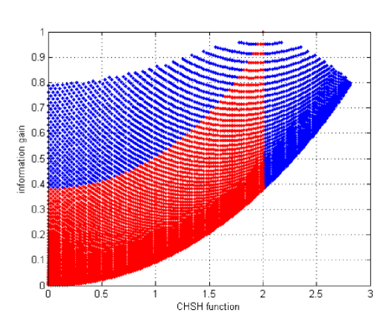
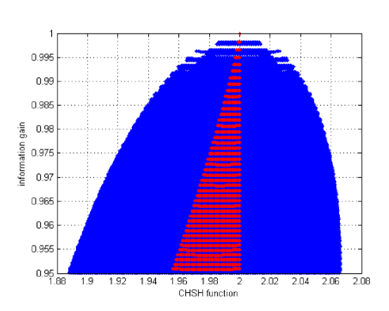
In our numerical calculations, we divide the defining domain of the joint probabilities $\Pr(B_{y}-A_{x}|x,y)$ into $100$ points. Follow the procedure of our brute-force method, we obtain the distribution of the information gain $I$ over the value of the CHSH function. The result is shown in Fig 3. for symmetric conditional probabilities $\Pr(\beta|a_{i},b=i)$ with i.i.d. and uniform input marginal probabilities $\Pr(a_{i})$. Note that, in Fig 3, all the points satisfy quantum constraint (76). We particularly use the red color to denote the points which also can be obtained by the local correlations, i.e., the value of the CHSH function and its three symmetric partners are all less than $2$. Moreover, it seems that the distribution of the information gain over the value of the CHSH function as shown in Fig 3 is not continuous. This is not the case but because we did not partition the defining domain of the joint probabilities fine enough.

In Fig 4 we partition more finely on the defining domain of the joint probabilities in the top region of Fig 3 and show that the empty region in Fig 3 is now filled. Similarly, the empty region on the top of Fig 4 could be filled again by the more fine partitioning.

The results in Fig 3 is consistent with the information causality since the maximal information gain for the local or quantum correlations is bound by 1, the bound suggested by information causality. However, the peculiar part of Fig 3 is that some of the local correlations can achieve the larger information gain than $I\simeq 0.8$, which is achieved by the correlations saturating the Tsireslon bound. This peculiar part is the red region above $I\simeq 0.8$ in Fig 3. Especially, the maximal information gain $I=1$ is reached when the shared correlation saturates the Bell inequality, i.e., the value of the CHSH function is equal to $2$. This indicates that the information gain is not monotonically related to the CHSH function. Or put this in the other way, the more amount of the quantum violation of Bell-type inequalities may not always yield the more information gain. We think it is interesting to understand this phenomenon in the future works.

Figure 5: Information gain vs the value of CHSH function for isotropic channels with i.i.d. and uniform input marginal probabilities.

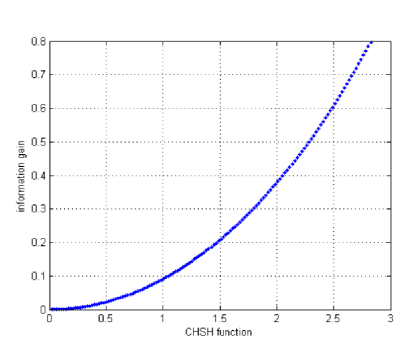
Form these symmetric conditional probabilities $\Pr(\beta|a_{i},b=i)$ realized quantum mechanically with i.i.d. and uniform input marginal probabilities $\Pr(a_{i})$, we pick up the isotropic ones ($\xi_{0}=\xi_{1}$) and obtain Fig 5. It shows that the information gain $I$ and the value of the CHSH function achieved by quantum mechanics are monotonically related. This explicitly demonstrate what we have discussed in the previous section.

2 Conditional probabilities with non-uniform input marginal probabilities

In the above conditional probabilities $\Pr(\beta|a_{i},b=i)$, the input marginal probabilities $\Pr(a_{i})$ are fixed to be i.i.d. and uniform $\Pr(a_{i})$. Now we would like to demonstrate the effect of non-uniform $\Pr(a_{i})$. In this case, we would like to vary $\Pr(a_{i})$ but keep the joint probabilities of the NS-box fixed. To see this effect for different conditional probabilities $\Pr(\beta|a_{i},b=i)$, we consider three different sets of the joint probabilities corresponding to (i) symmetric, (ii) symmetric and isotropic and (iii) asymmetric conditional probabilities $\Pr(\beta|a_{i},b=i)$.

To be more specific, for the case (i) the joint probabilities should be constrained by $\Pr(B_{y}-A_{x}=0|x,y=0)=1$ and $\Pr(B_{y}-A_{x}=xy|x,y=1)=\frac{1}{2}$ for $x=0,1$ such that the noise parameters are given by $\xi_{0}=1$ and $\xi_{1}=0$. For the case (ii) all the joint probabilities $\Pr(B_{y}-A_{x}=xy|x,y)$ are equal to $\frac{1}{2}(1+\frac{1}{\sqrt{2}})$ such that $\xi_{0}=\xi_{1}=\frac{1}{\sqrt{2}}$. For the case (iii) the joint probabilities are given by $\Pr(B_{y}-A_{x}=0|x=0,y)=\frac{1}{2}(1+\frac{1}{\sqrt{2}})$ and $\Pr(B_{y}-A_{x}=xy|x=1,y)=\frac{1}{2}$ for $y=0,1$. Obviously, it is asymmetric for general input marginal probabilities $\Pr(a_{i})$.

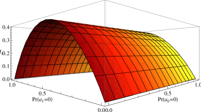
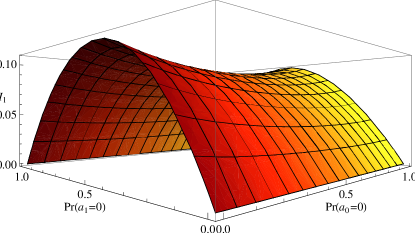
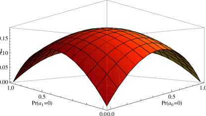
In the following discussion, we denote the mutual information $I(a_{0};\beta|b=0)$ as $I_{0}$ and $I(a_{1};\beta|b=1)$ as $I_{1}$, which are functions of two input marginal probabilities, namely, $\Pr(a_{0}=0)$ and $\Pr(a_{1}=0)$. Here $I_{i}$ can be thought as the mutual information between $a_{i}$ and $\beta$, and the corresponding noise parameter is $\xi_{i}$. The information gain $I$ is just $I=I_{0}+I_{1}$. Note that, $I_{0}$ does not depend on $\Pr(B_{y}-A_{x}=xy|x,y=1)$ and $I_{1}$ not on $\Pr(B_{y}-A_{x}=0|x,y=0)$. Thus, the conditional probabilities $\Pr(\beta|a_{0},b=0)$ for $I_{0}$ can be made symmetric by just requiring $\Pr(B_{y}-A_{x}=xy|x,y=0)$’s for $x=0,1$ are equal, and similarly for $\Pr(\beta|a_{1},b=1)$ for $I_{1}$ to be symmetric. An important feature for these symmetric conditional probabilities $\Pr(\beta|a_{0},b=0)$ is that $I_{i}$ will depend only on $\Pr(a_{i})$ not on $\Pr(a_{(i+1\mod 2)})$.

Figure 6: $I=I_{0}$ vs $\Pr(a_{0,1}=0$) for case (i).

Figure 7: Density plot of the Left figure.

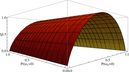
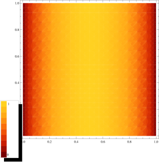
For case (i), conditional probabilities $\Pr(\beta|a_{i},b=i)$ $i=0,1$ are symmetric. Moreover, since $\xi_{0}=1$ and $\xi_{1}=0$ so that the corresponding channel between $a_{0}$ and $\beta$ for $\xi_{0}$ is noiseless and the corresponding channel between $a_{1}$ and $\beta$ for $\xi_{1}$ is completely noisy. This then leads to $I_{1}=0$ and $I=I_{0}$. The dependence of $I=I_{0}$ on one of the input marginal probabilities, i.e., $\Pr(a_{0}=0)$ only, is shown in Fig 7-7. Note that $I$ reaches its maximal value, $1$ at $\Pr(a_{0}=0)=\frac{1}{2}$ as expected for the symmetric conditional probabilities $\Pr(\beta|a_{0},b=0)$ with $\xi_{0}=1$. This point is nothing but the point of maximal $I$ in Fig 3. Note that this maximum saturates the bound by information causality. This implies that we can reach the causally-allowed bound on information gain by sacrificing one of the sub-set of the conditional probabilities, $\Pr(\beta|a_{1},b=1)$, without any comprise. This is a bit surprising.

Figure 8: $I_{0}$ vs $\Pr(a_{0,1}=0$) for case (ii).

Figure 9: $I_{1}$ vs $\Pr(a_{0,1}=0$) for case (ii).

Figure 10: $I$ vs $\Pr(a_{0,1}=0$) for case (ii).

Figure 11: Density plot of the Left figure.

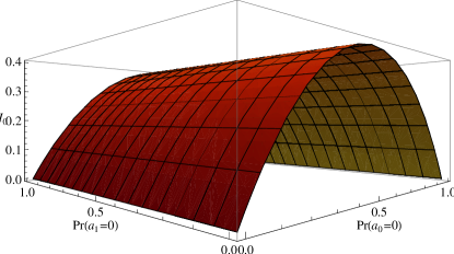
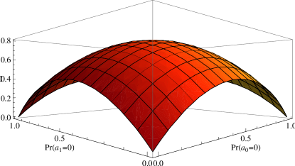
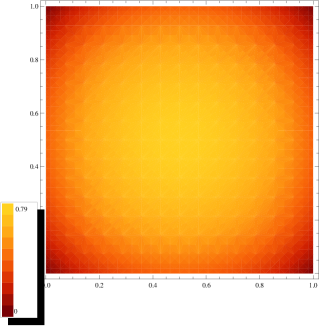
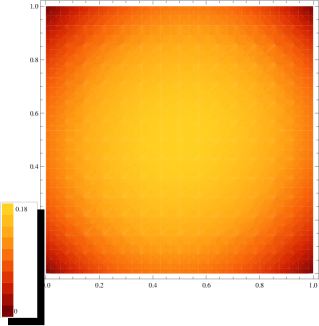
For case (ii), the conditional probabilities $\Pr(\beta|a_{i},b=i)$ for $i=0,1$ are both symmetric and isotropic, we then expect that the isotropy will also appear in the plot for $I$ vs the input marginal probabilities $\Pr(a_{i})$, and that $I_{0}$ and $I_{1}$ will have the same shape. This is indeed the case as shown in Fig 11-11. Note that $I_{i}$ only depends on $\Pr(a_{i})$ though $I=I_{0}+I_{1}$ depends on both. We see that the maximal value of $I$ occurs at the symmetric point, i.e., all the $Pr(a_{i})$ equal to $\frac{1}{2}$. However, the maximal value is $0.7983$ which is less than $1$ of the information causality but is the same value for the case of the Tsirelson bound.

Figure 12: $I_{0}$ vs $\Pr(a_{0,1}=0$) for case (iii).

Figure 13: $I_{1}$ vs $\Pr(a_{0,1}=0$) for case (iii).

Figure 14: $I$ vs $\Pr(a_{0,1}=0$) for case (iii).

Figure 15: Density plot of the Left figure.

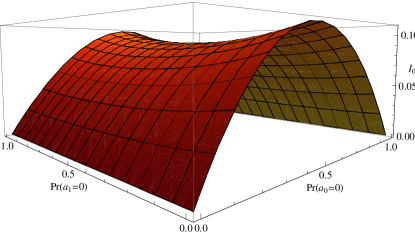
Finally, for case (iii), i.e., the particular asymmetric conditional probabilities $\Pr(\beta|a_{i},b=i)$, $I_{i}$’s are now dependent on both $\Pr(a_{i})$’s unlike in the previous two cases. However, the information gain $I$ has the isotropic form as in the case (ii) but with a far smaller maximal value at the symmetric point. The results are shown in Fig 15-15.

Our above results implies that the closer to $1$ is the $\Pr(B_{y}-A_{x}=xy|x,y)$, the larger is the information gain $I$. This is consistent with our RAC protocol as Bob can perfectly guess Alice’s inputs by using the PR box PRbox . Of course, the information causality ensures that the NS-box constrained by quantum mechanics can not be the PR box. Also, note that the maximum of $I$ occurs at the symmetric point of the input marginal probabilities $\Pr(a_{i})$ for case (ii) and (iii) but it is not the case for case (i). Therefore, the uniform input marginal probabilities $\Pr(a_{i})$ do not always lead to the maximal $I$.

3 Information causality for the most general conditional probabilities

After testing the information causality for the more general conditional probabilities $\Pr(\beta|a_{i},b=i)$ as discussed in the previous sections, we would wonder if the information causality holds for the most general conditional probabilities $\Pr(\beta|a_{i},b=i)$ or not, i.e., $\Pr(\beta|a_{i},b=i)$ without any additional constraint on the joint probabilities of the NS-box and the input marginal probabilities $\Pr(a_{i})$ except the necessary quantum and no-signaling constraints. For our $d=2$, $k=2$ RAC protocol, we check this by partitioning the defining domains of the probabilities into 100 points and then using the brute-force method to do the numerical check. We find that the information causality is always satisfied. This yields a more general support for the information causality.

Furthermore, we find that the information causality is saturated, i.e., $I=1$ when one of the sub-sets of conditional probabilities $\Pr(\beta|a_{i},b=i)$ corresponds to the noiseless channel between $a_{i}$ and $\beta$ and the other one corresponds to completely noisy channel. This is similar to the case (i) discussed in the previous subsection.

VI Conclusion

Information causality was proposed as a new physical principle and gives an intuitive picture on the meaning of causality from the information point of view. Therefore, to test its validity for general communication schemes will help to establish it as a physical principle. Motivated by this, in this work we try our best to extend the framework of the original proposal to the more general cases, such as the multi-level and multi-setting RAC protocols or lifting the symmetric and isotropic conditions on the conditional probabilities $\Pr(\beta|a_{i},b=i)$ or uniform condition on the input marginal probabilities $\Pr(a_{i})$. We then test the information causality for these general protocols by either adopting the SDP for numerical check, or using the brutal force method for the more general conditional probabilities $\Pr(\beta|a_{i},b=i)$. With all these efforts, our results are rewarding: we see that the information causality are preserved in all the protocols discussed in this work. This reinforce the validity of the information causality further than before. Though more checks for more general protocols should be always welcome. We also find that the information causality is saturated not by sharing the correlations saturating the Tsireslon bound, but by the ones which saturate the CHSH (or Bell) inequality. This then raises the issues on the intimate relation between the information gain and the quantum violation of the Bell-type inequalities. Especially, this result challenges our intuition that a channel can transfer more information by the quantum resources with the more amount of the violation of the Bell-type inequalities. We think our findings in this paper will shed some light on the related topics.

Appendix A Signal decay and data processing inequality for multi-nary channels

In this appendix, we will first sketch the key steps of Evans1 in obtaining the maximal bound on the signal decay for the binary noisy channels, and then generalize this derivation to the one for the multi-nary channels.

Our setup is to consider a cascade of two communication channels: $X\rightarrow Y\rightarrow Z$. The decay of the signal is implied by the data processing inequality, i.e.,

$$I(X;Z)\leq I(X;Y).$$ (77)

The mutual information $I(X;Y)=H(Y)-\sum_{i}\Pr(X=i)H(Y|X=i)$, where $H(Y)$ and $H(Y|X)$ are the Shannon entropies for the probabilities $\Pr(Y)$ and the conditional probabilities $\Pr(Y|X)$, respectively.

Furthermore, for the binary symmetric channel $A$ characterized by

$$A=\left({\begin{array}[]{cc}\frac{1+\xi}{2}&\frac{1-\xi}{2}\\ \frac{1-\xi}{2}&\frac{1+\xi}{2}\\ \end{array}}\right),$$ (80)

it was shown in Evans1 that the bound on the signal decay is characterized by the following bound

$$\frac{I(X;Z)}{I(X;Y)}\leq\xi^{2}.$$ (81)

Note that this bound is tighter than the one obtained in Pi , which is $\frac{I(X;Z)}{I(X;Y)}\leq\xi$.

In this appendix, we will generalize the above result to the one for the dinary channel characterized by $\Pr(Z=i|Y=i)=\xi$ and $\Pr(Z=s\neq i|Y=i)=\frac{1-\xi}{d-1}$ with $i\in\{0,1,...,d-1\}$, so that the signal decay is bound by

$$\frac{I(X;Z)}{I(X;Y)}\leq(\xi-\frac{1-\xi}{d-1})^{2}.$$ (82)

1 Sketch of the proof in Evans1

The derivation in Evans1 consists of two key steps. The first one is to show the following theorem for weak signal:

Theorem I: The ratio $\frac{I(X;Z)}{I(X;Y)}$ reaches its maximum if the conditional probabilities $\Pr(Y|X=0)$ and $\Pr(Y|X=1)$ are almost indistinguishable, i.e., $|\Pr(Y=0|X=0)-\Pr(Y=0|X=1)|\rightarrow 0$.

To prove this theorem we need the following lemma:

Lemma I: For any strictly concave function $f$ and $g$ on the interval $[0,1]$, and any $p\in[0,1]$, the ratio

$$r(x,y)=g_{2}(x,y,p)/f_{2}(x,y,p)$$ (83)

reaches its maximum in the limit $|x-y|\rightarrow 0$. Here $f_{2}(x,y,p)=f(px+(1-p)y)-pf(x)-(1-p)f(y)$ denotes the second order difference of the function $f$ with the weight $p$, and similarly for the $g_{2}(x,y,p)$.

We sketch the proof of this lemma, which will be useful when generalizing to the multi-nary channel. We assume that the ratio $r$ reaches its maximum at $x=x^{*}$ and $y=y^{*}$, and for concreteness assuming $x^{*}<y^{*}$. Note that $0<r<\infty$ due to the concave $f$ and $g$. We can perform affine transformation to scale this maximal value of $r(x^{*},y^{*},p)$ to be $1$, and also to make $f(x^{*})=g(x^{*})$ and $f(y^{*})=g(y^{*})$. This immediately leads to $f(px^{*}+(1-p)y^{*})=g(px^{*}+(1-p)y^{*})$. That is, there is a point $z^{*}=px^{*}+(1-p)y^{*}$ inside the interval $[x^{*},y^{*}]$ at which $f$ also equals to $g$. Use this fact, it is easy to convince oneself that either $r(z^{*},y^{*})\geq r(x^{*},y^{*})$ or $r(x^{*},z^{*})\geq r(x^{*},y^{*})$. For more subtle details, please see Evans1 . By repeating this procedure we prove the lemma.

Observe that $I(X;Y)$ and $I(X;Z)$ are the second order difference of the (concave) entropy functions $H(Y)$ and $H(Z)$, respectively with the weight $p=\Pr(X=0)$. We can then prove the Theorem I by the above lemma.

The second step is first to rewrite the ratio $\frac{I(X;Z)}{I(X;Y)}$ in terms of relative entropy $D(p\|q):=\sum_{x}\Pr(p=x)log\frac{\Pr(p=x)}{\Pr(q=x)}$, that is,

$$\frac{I(X;Z)}{I(X;Y)}=\frac{\sum_{i=0}^{1}\Pr(X=i)D(\Pr(Y|X=i)\cdot A\|\Pr(Y)\cdot A)}{\sum_{i=0}^{1}\Pr(X=i)D(\Pr(Y|X=i)\|\Pr(Y))}.$$ (84)

Then, based on the above theorem we can parameterize the conditional probabilities $\Pr(Y|X=0)=\vec{p}+\vec{\epsilon}$ where $\vec{p}=\sum_{i=0}^{1}\Pr(X=i)\Pr(Y|X=i)$ and $\vec{\epsilon}=(\epsilon,-\epsilon)$ with $\epsilon$ being sufficiently small. With this condition, (84) can be simplified to

$$\frac{I(X;Z)}{I(X;Y)}\approx\frac{D((\vec{p}+\vec{\epsilon})\cdot A\parallel\vec{p}\cdot A)}{D(\vec{p}+\vec{\epsilon}\parallel\vec{p})}.$$ (85)

Note that the ratio now does not depend on $\Pr(X)$.

Finally, given the binary channel (80) we can expand the relative entropy in terms of $\epsilon/\Pr(Y)$, so for the ratio $\frac{I(X;Z)}{I(X;Y)}$. Then, fixing $\epsilon$ and then varying the first order term of the ratio $\frac{I(X;Z)}{I(X;Y)}$ in the above expansion over $\vec{p}$, we obtain the bound in (81).

2 Generalizing to the multi-nary channels

We now generalize the above derivation to the trinary noisy channels, then the generalization to the dinary channel will just follows. The key steps are similar to the binary ones. The first step is to use the same method to prove the following theorem:

Theorem II: The ratio $\frac{I(X;Z)}{I(X;Y)}$ reaches its maximum only when all the three conditional probabilities $\Pr(Y|X=i)$ with $i=0,1,2$ are almost indistinguishable.

The strategy to prove this theorem is to observe that we can treat the pair $(\Pr(Y=0|X=i),\Pr(Y=1|X=i))$ for each $i$ (note that $\Pr(Y=2|X=i)$ is not independent of this pair) as a point inside the unit square $([0,1],[0,1])$. Then the three points $\Pr(Y|X=i)$ for $i=0,1,2$ form a triangle. We can then follow the same way of proving the Lemma I in the previous subsection for the trinary case. First, we assume the maximal value of $r$ occurs at all three vertices of some triangle. We then perform the affine transformation to rescale this maximal value to $1$, and to make $f=g$ (or more specifically $H(Y|X=i)=H(Z|X=i)$) at the three vertices of the above triangle. This then immediately leads to that there exists some point inside the triangle such that $f=g$. We can use this point to construct a smaller triangle with any two of the vertices of the original triangle and show that the ratio $r$ for this new triangle is greater than the one for the original larger triangle. Repeating this procedure we can prove the above theorem. It is also clear that we can generalize the theorem for the multi-nary channels by generalizing the triangle to the concave body of the higher dimensional space.

Here, we should point out that one can always reduce the concave body to the linear interval one, so that we can reduce to the situation for the binary case. That is, we set all the conditional probabilities except one to be equal, and then study the closeness condition of the remaining two distinct conditional probabilities for the maximal ratio of $\frac{I(X;Z)}{I(X;Y)}$. In the following, we will always restrict to such a situation.

We then go to the second step as for the binary channel, that is to use Theorem II to reduce the problem of maximizing $\frac{I(X;Z)}{I(X;Y)}$ to the one of maximizing the ratio of relative entropies. We rewrite the ratio of two mutual information as following,

$$\frac{I(X;Z)}{I(X;Y)}=\frac{\sum_{i=0}^{2}\Pr(X=i)D(\Pr(Y|X=i)\cdot A\|\Pr(Y)\cdot A)}{\sum_{i=0}^{2}\Pr(X=i)D(\Pr(Y|X=i)\|\Pr(Y))}.$$ (86)

To simplify the expression for further manipulations, we denote the average probability distribution of $Y$ as $\vec{p}=\sum_{i=0}^{2}\Pr(X=i)\Pr(Y|X=i)$, and parameterize the probability $\Pr(Y|X=0)=\vec{p}+\vec{\epsilon}_{0}$ and $\Pr(Y|X=1)=\vec{p}+\vec{\epsilon}_{1}$. Thus, the probability $\Pr(Y|X=2)$ is forced to be $\vec{p}-\frac{\Pr(X=0)}{\Pr(X=2)}\vec{\epsilon}_{0}-\frac{\Pr(X=1)}{\Pr(X=2)}\vec{\epsilon}_{1}$. The parameter vectors $\vec{\epsilon}_{0}$ and $\vec{\epsilon}_{1}$ should be sufficiently small as required by Theorem II to have maximal ratio $\frac{I(X;Z)}{I(X;Y)}$. Furthermore, we will further reduce the triangle to the linear interval case by assuming $\vec{\epsilon}_{0}=\vec{\epsilon}_{1}$, i.e., $\Pr(Y|X=0)=\Pr(Y|X=1)$.

The ratio (86) then becomes

$$\frac{I(X;Z)}{I(X;Y)}\approx\frac{D((\vec{p}+\vec{\epsilon_{0}})\cdot A\parallel\vec{p}\cdot A)}{D(\vec{p}+\vec{\epsilon_{0}}\parallel\vec{p})}.$$ (87)

Note again the ratio now does not depend on $\Pr(X)$.

Before serious expansion of (87) in the power of $\vec{\epsilon}_{0}$, we need to specify $\vec{p}=({\scriptstyle\Pr(Y=0),\Pr(Y=1),\Pr(Y=2)})$ and $\vec{\epsilon}_{0}=({\scriptstyle v_{0},v_{1},v_{2}})$. Note that, $v_{0}+v_{1}+v_{2}=0$. As for the bi-nary channel, we expand the relative entropy in terms of $\frac{v_{i}}{\Pr(Y=i)}$. The leading term of the expansion for the denominator of (87) is found to be

$$D(\vec{p}+\epsilon_{0}\parallel\vec{p})=\frac{1}{2ln2}\sum_{i=0}^{1}\frac{v_{i}^{2}}{\Pr(Y=i)}.$$ (88)

To find the expansion of the numerator, we need to specify the channel $A$ between $Y$ and $Z$. The generic trinary channel is given by

$$A=\Pr(Z|Y)=\left({\begin{array}[]{ccc}a_{1}&a_{2}&a_{3}\\ b_{1}&b_{2}&b_{3}\\ c_{1}&c_{2}&c_{3}\end{array}}\right),$$ (92)

where the elements of the channel should satisfy $a_{1}+a_{2}+a_{3}=1$, $b_{1}+b_{2}+b_{3}=1$, and $c_{1}+c_{2}+c_{3}=1$. Then, the leading term in the expansion of the numerator of (87) is found to be

$${\textstyle D((\vec{p}+\vec{\epsilon_{0}})\cdot A\parallel\vec{p}\cdot A)=\frac{1}{2ln2}(\frac{v_{0}a_{1}+v_{1}b_{1}+v_{2}c_{1}}{p(Z=0)}+\frac{v_{0}a_{2}+v_{1}b_{2}+v_{2}c_{2}}{p(Z=1)}+\frac{v_{0}a_{3}+v_{1}b_{3}+v_{2}c_{3}}{p(Z=2)})}.$$ (93)

For simplicity, we only consider the symmetry trinary channel as follows

$$A=\Pr(Z|Y)=\left({\begin{array}[]{ccc}\xi&\frac{1-\xi}{2}&\frac{1-\xi}{2}\\ \frac{1-\xi}{2}&\xi&\frac{1-\xi}{2}\\ \frac{1-\xi}{2}&\frac{1-\xi}{2}&\xi\end{array}}\right).$$ (97)

Then, (93) then becomes

$$D((\vec{p}+\vec{\epsilon_{0}})\cdot A\parallel\vec{p}\cdot A)=(\frac{3\xi-1}{2})^{2}\frac{1}{2ln2}\sum_{i=0}^{2}\frac{v_{i}^{2}}{\Pr(Z=i)}.$$ (98)

Since we know that for symmetric channel, the maximal mutual information is achieved for uniform input probabilities. Thus, we assume uniform $\Pr(Y)$ and $\Pr(Z)$ so that (87) depends only on variable $\xi$. We then obtain

$$\frac{I(X;Z)}{I(X;Y)}\leq(\frac{3\xi-1}{2})^{2}.$$ (99)

This is the generalization of (81) for binary channel to the trinary one.

Similarly, we can generalize the above derivation to the dinary channels. If the channel between $Y$ and $Z$ is a dinary and symmetry channel specified as follows: $\Pr(Z=i|Y=i)=\xi$ and $\Pr(Z=s\neq i|Y=i)=\frac{1-\xi}{d-1}$ with $i\in\{0,1,...,d-1\}$, then the bound of the ratio $\frac{I(X;Z)}{I(X;Y)}$ is given by (82).

Appendix B The concavity of information gain

In this appendix, we want to prove the information gain $I$ is not a concave function to joint probabilities $\Pr(B_{\vec{y}}-A_{\vec{x}}|\vec{x},\vec{y})$ and input marginal probabilities $\Pr(a_{i})$. Thus, we could not formulate the problem (maximizing information gain $I$) as a convex optimization programming.

First, we re-express information gain $I$ by $\Pr(B_{\vec{y}}-A_{\vec{x}}|\vec{x},\vec{y})$ and $\Pr(a_{i})$. If maximizing information gain is a concave function to these probabilities, the second order partial derivative of mutual information respecting to each probability should be negative. Here, we find a violation when calculating $\frac{\partial^{2}I}{\partial(\Pr(B_{\vec{y}}-A_{\vec{x}}=0|\vec{x}=0,\vec{y}=0))^{2}}$. In following paragraphs, we denote the joint probabilities $\Pr(B_{\vec{y}}-A_{\vec{x}}=0|\vec{x}=0,\vec{y}=0)$ as $V$.

The information gain can be rewritten as

$$I=\sum_{i=0}^{k-1}I_{b=i},$$ (100)

where $I_{b=i}$ is equal to $I(a_{i};\beta|b=i)$. Since the joint probability $V$ only contribute to $I_{b=0}$, we only need to calculate $\frac{\partial^{2}I_{b=0}}{\partial V^{2}}$. The reexpression of $I_{b=0}$ is

$$I_{b=0}=\sum_{n=0}^{d-1}\sum_{j=0}^{d-1}\Pr(\beta=n,a_{0}=j|b=0)log_{2}\frac{\Pr(\beta=n,a_{0}=j|b=0)}{\Pr(\beta=n|b=0)\Pr(a_{0}=j|b=0)}.$$ (101)

Therefore, the first order partial derivative respecting to $\Pr(B_{\vec{y}}-A_{\vec{x}}=0|\vec{x}=0,\vec{y}=0)$ is

$$\frac{\partial I_{b=0}}{\partial V}=$$

$$\sum_{n=0}^{d-1}\sum_{j=0}^{d-1}\frac{\partial\Pr(a_{0}=j,\beta=n|b=0)}{\partial V}log_{2}\frac{\Pr(a_{0}=j,\beta=n|b=0)}{\Pr(\beta=n|b=0)\Pr(a_{0}=j|b=0)}$$

$$+\frac{1}{ln2}(\frac{\partial\Pr(a_{0}=j,\beta=n|b=0)}{\partial V}-\frac{\Pr(a_{0}=j,\beta=n|b=0)}{\Pr(\beta=n|b=0)}\frac{\partial\Pr(\beta=n|b=0)}{\partial V})$$ (102)

We can express $\Pr(a_{0}=j,\beta=n|b=0)$ as the combination of joint probabilities $\Pr(B_{\vec{y}}-A_{\vec{x}}|\vec{x},\vec{y})$ and input marginal probabilities $\Pr(a_{i})$ to obtain $\frac{\partial\Pr(a_{0}=j,\beta=n|b=0)}{\partial V}$.
Since joint probabilities $\Pr(B_{\vec{y}}-A_{\vec{x}}|\vec{x},\vec{y})$ are subjected to the normalization conditions of total probability, if $n-j\neq(d-1)$,

$${\scriptstyle\Pr(a_{0}=j,\beta=n|b=0)=\sum_{a_{k\neq 0}}\Pr(B_{\vec{y}}-A_{\vec{x}}=n-j|\vec{x},\vec{y}=0)\Pr(a_{0}=j)\;\Pi_{k\neq 0}\Pr(a_{k})};$$ (103)

if $n-j=(d-1)$,

$${\scriptstyle\Pr(a_{0}=j,\beta=n|b=0)=\sum_{a_{k\neq 0}}(1-\sum_{t=0}^{d-2}\Pr(B_{\vec{y}}-A_{\vec{x}}=t|\vec{x},\vec{y}=0))\Pr(a_{0}=j)\;\Pi_{k\neq 0}\Pr(a_{k})},$$ (104)

where $\vec{x}$ in the above functions is given by the RAC encoding, i.e., $\vec{x}:=(x_{1},\cdots,x_{k-1})$ with $x_{i}=a_{i}-a_{0}$

Now, we can calculate the derivatives. The patrial derivative

$$\frac{\partial\Pr(a_{0}=j,\beta=n|b=0)}{\partial V}$$ (105)

is not equal to zero for two cases, the first one is $j=n$, we can obtain $\;\Pi_{k}\Pr(a_{k}=n)$ for (105). The second case is $n-j=(d-1)$, we can obtain $\;-\Pi_{k}\Pr(a_{k}=n-(d-1))$. Therefore, since $\Pr(\beta=n|b=0)=\sum_{j}\Pr(a_{0}=j,\beta=n|b=0)$, we can obtain

$$\frac{\partial\Pr(\beta=n|b=0)}{\partial V} =\Pi_{k}\Pr(a_{k}=n)-\Pi_{k}\Pr(a_{k}=n-(d-1)).$$ (106)

Put above result to (B), for fixed $j$, we can find that $\sum_{n=0}^{d-1}\frac{\partial\Pr(a_{0}=j,\beta=n|b=0)}{\partial V}=0$, thus the second term of (B) will vanish.

We then can calculate the second order derivative

$$\frac{\partial^{2}I_{b=0}}{\partial V^{2}}=\frac{1}{ln2}\sum_{n=0}^{d-1}\sum_{j=0}^{d-1}(\frac{\partial\Pr(a_{0}=j,\beta=n|b=0)}{\partial V})^{2}\frac{1}{\Pr(a_{0}=j,\beta=n|b=0)}$$

$$-\frac{2}{\Pr(\beta=n|b=0)}\frac{\partial\Pr(a_{0}=j,\beta=n|b=0)}{\partial V}\frac{\partial\Pr(\beta=n|b=0)}{\partial V}+(\frac{\partial\Pr(\beta=n|b=0)}{\partial V})^{2}\frac{\Pr(a_{0}=j,\beta=n|b=0)}{(\Pr(\beta=n|b=0))^{2}}$$ (107)

For $d=2$ and $k=2$, (B) becomes

$$\frac{\partial^{2}I}{\partial V^{2}}=\frac{1}{ln2}[(\Pr(a_{0}=0)\Pr(a_{1}=0))^{2}(\frac{1}{\Pr(a_{0}=0,\beta=0|b=0)}+\frac{1}{\Pr(a_{0}=0,\beta=1|b=0)})$$

$$+(\Pr(a_{0}=1)\Pr(a_{1}=1))^{2}(\frac{1}{\Pr(a_{0}=1,\beta=0|b=0)}+\frac{1}{\Pr(a_{0}=1,\beta=1|b=0)})$$

$$-(\frac{1}{\Pr(\beta=0|b=0)}+\frac{1}{\Pr(\beta=1|b=0)})(\Pr(a_{0}=0)\Pr(a_{1}=0)-\Pr(a_{0}=1)\Pr(a_{1}=1))^{2}]$$

Once $\Pr(a_{0}=0)=1-\Pr(a_{1}=0)$, the above function is non-negative.

For higher $d$ and $k$, once the input marginal probabilities $\Pr(a_{i})$ are uniform. We then can obtain

$$\frac{\partial^{2}I}{\partial V^{2}}=\frac{\partial^{2}I_{b=0}}{\partial V^{2}}=$$

$$\frac{1}{ln2}\sum_{n=0}^{d-1}\frac{1}{d^{2k}}(\frac{1}{\Pr(a_{0}=n,\beta=n|b=0)}+\frac{1}{\Pr(a_{0}=n,\beta=n-(d-1)|b=0)})$$

$$>0$$ (109)

It is clear that information gain $I$ is not a concave function to joint probabilities $\Pr(B_{\vec{y}}-A_{\vec{x}}|\vec{x},\vec{y})$ and input marginal probabilities $\Pr(a_{i})$.

Appendix C Semidefinite programming

In this appendix, we briefly introduce the semidefinite programming (SDP) SDP . SDP is the problem of optimizing a linear function subjected to certain conditions associated with a positive semidefinite matrix $X$, i.e., $v^{{\dagger}}Xv\geq 0$, for $v\in\mathbb{C}^{n}$, and is denoted by $X\succeq 0$. It can be formulated as the standard primal problem as follows. Given the $n\times n$ symmetric matrices $C$ and $D_{q}$’s with $q=1,\cdots,m$, we like to optimize the $n\times n$ positive semidefinite matrix $X\succeq 0$ such that we can achieve the following:

$$minimize\qquad \mbox{Tr}(C^{T}X)$$ (110a)

$$subject\quad to\qquad \mbox{Tr}(D_{q}^{T}X)=b_{q},\quad q=1,\cdots,m\;.$$ (110b)

Corresponding to the above primal problem, we can obtain a dual problem via a Lagrange approach CV . The Lagrange duality can be understood as the following. If the primal problem is

$$minimize\qquad f_{0}(x)$$ (111a)

$$s.t.\qquad f_{q}(x)\leq 0,\quad q\in 1...m.$$ (111b)

$$h_{q}(x)=0,\quad q\in 1...p,$$ (111c)

the Lagrange function can be defined as

$$L(x,\lambda,\nu)=f_{0}(x)+\Sigma_{q=1}^{m}\lambda_{q}f_{q}(x)+\Sigma_{q=1}^{p}\nu_{q}h_{q}(x),$$ (112)

where $\lambda_{1}$,…, $\lambda_{m}$, and $\nu_{1}$,…,$\nu_{p}$ are Lagrange multipliers respectively. Due to the problem and (112), the minima of $f_{0}$ is bounded by (112) under the constraints when $\lambda_{1}$,…, $\lambda_{m}\geq 0$.

$$\mathop{\inf}_{x}f_{0}\geq\mathop{\inf}_{x}L(x,\lambda,\nu).$$

Then the Lagrange dual function is obtained.

$$g(\lambda,\nu)=\mathop{\inf}_{x}L(x,\lambda,\nu).$$

$g(\lambda,\nu)\leq p$ ($p$ is the optimal solution of $f_{0}(x)$ ), for $\lambda_{1}$,…, $\lambda_{m}\geq 0$ and arbitrary $\nu_{1}$,…,$\nu_{p}$. The dual problem is defined.

$$maximize\qquad g(\lambda,\nu)$$ (113a)

$$s.t.\qquad \lambda_{q}\geq 0.\quad(q\in\{1...m\})$$ (113b)

We can use the same method to define the dual problem for SDP. From the primal problem of SDP (110), we can write down the dual function by using minimax inequality DPP .

$$\mathop{\inf}_{X\succeq 0}\mbox{Tr}(C^{T}X) =\mathop{\inf}_{X\succeq 0}\mbox{Tr}(C^{T}X)+\sum_{q=1}^{m}y_{q}(b_{q}-\mbox{Tr}(D_{q}^{T}X))$$

$$=\mathop{\inf}_{X\succeq 0}\mathop{\sup}_{y}\sum_{q=1}^{m}y_{q}(b_{q})+\mbox{Tr}((C^{T}-\sum_{q=1}^{m}y_{q}D_{q}^{T})X)$$

$$\geq\mathop{\sup}_{y}\mathop{\inf}_{X\succeq 0}\sum_{q=1}^{m}y_{q}(b_{q})+\mbox{Tr}((C^{T}-\sum_{q=1}^{m}y_{q}D_{q}^{T})X)$$

$$=\mathop{\sup}_{y}\mathop{\inf}_{X\succeq 0}\sum_{q=1}^{m}y_{q}(b_{q})+\mbox{Tr}((C-\sum_{q=1}^{m}y_{q}D_{q})^{T}X).$$ (114)

The optimal solution of dual function is bounded under some vector $y$.

$$\mathop{\sup}_{y}\mathop{\inf}_{X\succeq 0}\sum_{q=1}^{m}y_{q}(b_{q})+\mbox{Tr}((C-\sum_{q=1}^{m}y_{q}D_{q})^{T}X)=\left\{\begin{array}[]{l}\mathop{\sup}_{y}\sum_{q=1}^{m}y_{q}(b_{q})\quad;when\quad C-\sum_{q=1}^{m}y_{q}D_{q}\succeq 0\\ -\infty\qquad;otherwise.\end{array}\right.$$ (116)

The correspond dual problem is

$$maximize\qquad \sum_{q=1}^{m}y_{q}(b_{q})$$ (117a)

$$s.t.\qquad S=C-\sum_{q=1}^{m}y_{q}D_{q}\succeq 0.$$ (117b)

If the feasible solutions for the primal problem and the dual problem attain their minimal and maximal values denoted as $p^{\prime}$ and $d^{\prime}$ respectively, then $p^{\prime}\geq d^{\prime}$, which is called the duality gap. This implies that the optimal solution of primal problem is bounded by dual problem. This then leads to the following: Both the primal and the dual problems attain their optimal solutions when the duality gap vanishes, i.e., $d^{\prime}=p^{\prime}$.

Appendix D The quantum constraints for $n=1$ and $n=1+AB$ certificate

We divide this appendix into two parts. In the first part, we will write down the associated quantum constraints for $\Gamma^{(1)}$ and $\Gamma^{(1+AB)}$ when finding the bound of the Bell-type functions. In the second part, we will estimate the number of these constraints and find a efficient way to write down these constraints.

1 The quantum constraints for $n=1$ and $n=1+AB$ certificate

When maximizing the Bell-type inequalities under some quantum constraints, the joint probabilities are not given, they are variables. Therefore, when writing down quantum constraints (58b), we only need to consider the elements with the specific value ($0$ and $1$) and the relation between different elements such as some elements are the same. For convenience, instead of $A_{\vec{x}}$ and $B_{\vec{y}}$, we use $a:a\in\tilde{A}$ and $b:b\in\tilde{B}$ to denote Alice’s and Bob’s outcomes and $X(a)$ and $Y(b)$ are the associated measurement setting. The indexes $s,t$ of $\Gamma$ denote associated operators, i.e., $\Gamma_{a,b}=\mbox{Tr}(E_{a}E_{b}\rho)$.

For $\Gamma^{(1)}$, the associated quantum constraints are

• $\Gamma^{(1)}_{1,1}=\mbox{Tr}(\rho)=1$.

• $\Gamma^{(1)}_{a,a^{\prime}}=\delta_{aa^{\prime}}\Gamma^{(1)}_{1,a}$ if $X(a)=X(a^{\prime})$.

• $\Gamma^{(1)}_{b,b^{\prime}}=\delta_{bb^{\prime}}\Gamma^{(1)}_{1,b}$ if $Y(a)=Y(a^{\prime})$.

• $\Gamma^{(1)}_{s,t}=\Gamma^{(1)}_{t,s}$.

We reexpress $\Gamma^{(1+AB)}$ by $4$ sub-matrixes,

$$\left(\begin{array}[]{cc}v_{1,1}&v_{1,2}\\ v_{2,1}&v_{2,2}\\ \end{array}\right)$$ (120)

Since $\Gamma^{(1+AB)}$ is symmetric matrix, the sub-matrix $v_{2,1}$ is equal to the transpose of $v_{1,2}$, and both sub-matrix $v_{1,1}$ and $v_{2,2}$ are symmetric matrixes. Note that, $v_{1,1}=\Gamma^{(1)}$. The elements of matrices $v_{1,2}$ and $v_{2,2}$ are constrained by following quantum constrains:

• $\Gamma^{(1+AB)}_{1,ab}=\Gamma^{(1+AB)}_{a,ab}=\Gamma^{(1+AB)}_{a,b}=\Gamma^{(1+AB)}_{b,ab}$.

• $\Gamma^{(1+AB)}_{ab,a^{\prime}b}=\Gamma^{(1+AB)}_{a,a^{\prime}b}=\Gamma^{(1+AB)}_{a^{\prime},ab}$.

• $\Gamma^{(1+AB)}_{ab,ab^{\prime}}=\Gamma^{(1+AB)}_{b,ab^{\prime}}=\Gamma^{(1+AB)}_{b^{\prime},ab}$.

• $\Gamma^{(1+AB)}_{a,a^{\prime}}=0$, $\Gamma^{(1+AB)}_{a,a^{\prime}b}=0$, and $\Gamma^{(1+AB)}_{ab,a^{\prime}b^{\prime}}=0$ if $X(a^{\prime})=X(a)$.

• $\Gamma^{(1+AB)}_{b,b^{\prime}}=0$, $\Gamma^{(1+AB)}_{b,ab^{\prime}}=0$, and $\Gamma^{(1+AB)}_{ab,a^{\prime}b^{\prime}}=0$ if $Y(b)=Y(b^{\prime})$.

• $\Gamma^{(1+AB)}_{s,t}=\Gamma^{(1+AB)}_{t,s}$.

2 Estimating the number of constrains for $n=1$ and $n=1+AB$ certificates

Due to the limitation of computer memory, we need to estimate the number of these quantum constraints for different $k$ and $d$ RAC protocols. The dimension of $\Gamma^{(1)}$ is $1+(d-1)(d^{k-1}+k)$, we denote it as $dim$. The number of conditions corresponding to different quantum behaviors is as follows.

n=1	symmetric matrix	$\mbox{Tr}(\rho)=\Gamma^{(1)}_{1,1}=1$	orthogonality	$E_{a}E_{a}=E_{a},E_{b}E_{b}=E_{b}$
number	$\frac{dim(dim-1)}{2}$	$1$	$\frac{(d-1)(d-2)}{2}(d^{k-1}+k)$	$dim-1$

The dimension of $\Gamma^{(1+AB)}$ is $1+(d-1)(d^{k-1}+k)+(d-1)(d^{k-1}k)$, we denote it as $dim_{1+AB}$. The number of conditions corresponding to different quantum behaviors is as follows.

n=1+AB	symmetric matrix	$Tr(\rho)=\Gamma^{1}_{1,1}=1$	orthogonality	$E_{a}E_{a}=E_{a},E_{b}E_{b}=E_{b}$	same
number	$\frac{dim_{1+AB}(dim_{1+AB}-1)}{2}$	1	$otha+othb+othc$	$dim_{1+AB}-1$	$\sum_{i=1}^{7}same_{i}$

The quantum constraints orthogonality and commutativity make some elements of certificate to be $0$ or to be the same. We will specify to estimate the number of these special elements in $n=1+AB$ certificate. First, we estimate the number of elements whose value is zero.

• The variable $otha=\frac{(d-1)(d-2)}{2}(d^{k-1}+k)$ is used to specify the number of zero elements for right upper matrix of $v_{1,1}$.

• The variable $othb=2(d-1)^{2}(d-2)kd^{k-1}$ is used to specify the number of zero elements for sub-matrix $v_{1,2}$.

• The variable $othc=\frac{kd^{k-1}(d-1)^{2}}{2}((d-2)(d-1)(d^{k-1}+k-2)+(d-1)^{2}-1)$ is used to specify the number of zero elements for right upper matrix of $v_{2,2}$.

We estimate the variable $same_{i}$ which is used to denote the number of equal pairs.

• $\Gamma^{(1+AB)}_{1,ab}=\Gamma^{(1+AB)}_{a,ab}$, $same_{1}=(d-1)^{2}(d^{k-1}k)$.

• $\Gamma^{(1+AB)}_{a,ab}=\Gamma^{(1+AB)}_{a,b}$, $same_{2}=(d-1)^{2}(d^{k-1}k)$.

• $\Gamma^{(1+AB)}_{b,ab}=\Gamma^{(1+AB)}_{a,b}$, $same_{3}=(d-1)^{2}(d^{k-1}k)$.

• $\Gamma^{(1+AB)}_{ab,a^{\prime}b}=\Gamma^{(1+AB)}_{a,a^{\prime}b}$, $same_{4}=(d-1)^{3}d^{k-1}k(d^{k-1}-1)/2$.

• $\Gamma^{(1+AB)}_{a,a^{\prime}b}=\Gamma^{(1+AB)}_{a^{\prime},ab}$, $same_{5}=(d-1)^{3}d^{k-1}k(d^{k-1}-1)$.

• $\Gamma^{(1+AB)}_{ab,ab^{\prime}}=\Gamma^{(1+AB)}_{b,ab^{\prime}}$, $same_{6}=(d-1)^{3}d^{k-1}k(k-1)/2$.

• $\Gamma^{(1+AB)}_{b,ab^{\prime}}=\Gamma^{(1+AB)}_{b^{\prime},ab}$, $same_{7}=(d-1)^{3}d^{k-1}k(k-1)$.

After estimating the number of conditions, we can think how to write down these conditions with minimal computer memory. Here, we use the numerical package named CVXOPT CVXOPT to calculate the bounds of the Bell-type inequalities. The primal problem of the cone programming defined in CVXOPT is

$$minimize\qquad c\cdot x$$ (121a)

$$subject\quad to\qquad Ax-b=0$$ (121b)

$$h-Gx\geq 0$$ (121c)

Given $c$, $h$ which are the vectors and $A$, $G$ which are matrixes, we can optimize the linear combination $c\cdot x$. Here matrix $G$ is used to specify the positive definiteness constraint. Writing down the positive definiteness constraint of a matrix $Z$ whose size is $s\times s$, we need the matrix $G$ with size $s^{2}\times n$ to define the condition (where $n$ is the number of variables $x$). That means, if we reduce the number of variables, we can save the computer memory. To do this, we define the same variable for two elements instead of constraining two variables with the same value. On the other hand, if the value of some elements are zero, it could also reduce the number of variables.

After using the conditions to reduce the number of variables, we can estimate the number of variables in the certificate.
The number of variables in $\Gamma^{(1)}$ for different RAC protocols:

n=1	d=2	d=3	d=4	d=5
k=2	10	50	153	364
k=3	28	288	1596	6160
k=4	78	1922	20706	132612

The number of variables in $\Gamma^{(1+AB)}$ for different RAC protocols:

n=1+AB	d=2	d=3	d=4	d=5
k=2	15	182	1287	5964
k=3	82	4068	61860	474160
k=4	486	71258	1995810	24012612

Due to the constraint of the computer memory (128GB), we could not find the bounds of the Bell-type inequalities for arbitrary RAC communication protocols. We find the bound what we can do and show the result in the main text.

References

- (1) H. Buhrman, R. Cleve, S. Massar and R. de Wolf, “Nonlocality and communication complexity”, Rev. Mod. Phys. vol. 82, 665 (2010).
- (2) van Dam W. “Implausible consequences of superstrong nonlocality”, arXiv:quant-ph/0501159v1.
- (3) S. Popescu and D. Rohrlich, “Nonlocality as an axiom”, Found. Phys. 24 379 (1994).
- (4) M. Pawlowski, T. Paterek, D. Kaszlikowski, V. Scarani, A. Winter, and M. Zukowski, “Information causality as a physical principle”, Nature, 461, 1101 (2009).
- (5) L. -Y. Hsu, I-C. Yu and F. -L. Lin, “Information Causality and Noisy Computations”, Phys. Rev. A 84, 042319 (2011).
- (6) Jon Barrett, Noah Linden, S. Massar, S. Pironio, Sandu Popescu, and D. Roberts, “Non-local correlations as an information-theoretic resource,” Physical Review A, 795:140401, 2005. Jon Barrett and Stefano Pironio, “Popescu-Rohrlich correlations as a unit of nonlocality,” Physical Review Letters, A456:1175 1182, 2005.
- (7) Navascues M. and Wunderlich H., “A glance beyond the quantum model”,(2009) Proc. R. Soc. A 466, 881.
- (8) D. Cavalcanti, A. Salles and V. Scarani, “Macroscopically local correlations can violate information causality”, Nat. Comm. 1, 136 (2010). [arXiv:1008.2624 [quant-ph]].
- (9) Oscar C. O. Dahlsten, D. Lercher and R. Renner. “Tsirelson’s bound from a generalized data processing inequality”, New J. Phys. 14, 063024 (2012).
- (10) Sabri W. Al-Safi and Anthony J. Short, “Information causality from an entropic and a probabilistic perspective”, Phys. Rev. A 84, 042323 (2011).
- (11) W. Evans and L. J. Schulman, “Signal Propagation, with Application to a Lower Bound on the Depth of Noisy Formulas”, Proceedings of the 34th Annual Symposium on Foundations of Computer Science, 594 (1993).
- (12) W. Evans and L. J. Schulman, “Signal Propagation and Noisy Circuits”, IEEE Trans. Inf. Theory, 45, 2367 (1999).
- (13) N. Pippenger. Reliable computation by formulas in the presence of noise. IEEE Tkansactions on Information Theory, 34(2):194-197, March 1988.
- (14) B. S. Tsirelson, “Quantum analogues of the Bell inequalities”, J. Sov. Math. 36, 557 (1987).
- (15) L. J. Landau, “Empirical two-point correlation functions”, Found. Phys. 18, 449 (1988).
- (16) B. Tsirelson, “Some results and problems on quantum Bell-type inequalities.”, Hadronic J. Suppl. 8, 329 (1993).
- (17) L. Masanes, “Necessary and sufficient condition for quantum-generated correlations”, quant-ph/0309137.
- (18) S. Wehner, “Tsirelson bounds for generalized Clauser-Horne-Hold inequalities”, Phys. Rev. A 73, 022110 (2006).
- (19) M. Navascues, S. Pironio, and A. Acin, “Bounding the set of quantum correlations”, Phys. Rev. Lett. 98, 010401 (2007).
- (20) M. Navascues, S. Pironio, A. Acin, “A convergent hierarchy of semidefinite programs characterizing the set of quantum correlations”, New J. Phys. 10, 073013 (2008).
- (21) http://abel.ee.ucla.edu/cvxopt/ .
- (22) T. M. Cover and J. A. Thomas, Elements of Information Theory. New York: Wiley, 1991.
- (23) Singiresu S. Rao, Engineering Optimization: Theory and Practice, Fourth Edition, John Wiley , Sons, Inc, 2009.
- (24) L. Vandenberghe and S. Boyd, SIAM Review 38, 1 (1996).
- (25) S. Boyd and L. Vandenberghe(2004). “Convex Optimization”, Cambridge University Press.
- (26) R. A. Horn and C. R. Johnson, “Matrix Analysis”, Cambridge University Press, New York, 1990.