Object-oriented Bayesian networks for a decision support system for antitrust enforcement

Abstract

We study an economic decision problem where the actors are two firms and the Antitrust Authority whose main task is to monitor and prevent firms’ potential anti-competitive behaviour and its effect on the market. The Antitrust Authority’s decision process is modelled using a Bayesian network where both the relational structure and the parameters of the model are estimated from a data set provided by the Authority itself. A number of economic variables that influence this decision process are also included in the model. We analyse how monitoring by the Antitrust Authority affects firms’ strategies about cooperation. Firms’ strategies are modelled as a repeated prisoner’s dilemma using object-oriented Bayesian networks. We show how the integration of firms’ decision process and external market information can be modelled in this way. Various decision scenarios and strategies are illustrated.

T1Supported by a PRIN07 Italian Research Grant. Sections 3.1, 4.1 and 4.3 are due to C. Vergari, the remaining sections are due to J. Mortera and P. Vicard.

, and

1 Introduction

Firms in many cases have incentives to cooperate (collude) to increase their profits. The possibility for firms to collude does not depend solely on their decision but also on external circumstances. First of all, firms need to comply with antitrust laws. If the Antitrust Authority (AA) finds negative anti-competitive effects, resulting from firms’ cooperative behaviour, it may intervene to prevent the firms from merging.

The AAs decision process is modelled here by using a Bayesian network (BN) or Probabilistic Expert System (PES) [Cowell et al. (1999)] estimated from real data. A BN is a graphical model that encodes the probabilistic relationships among the variables of interest allowing for the application of fast general-purpose algorithms to compute inferences.

Often governments may find negative anti-competitive effects resulting from a merger. As a consequence, the decision by firms to cooperate is actually affected by the decision process of the AA. The AA may start an investigation either because two firms make a formal request to merge (explicit collusion) or because the authority suspects that two firms are implicitly colluding. In what follows the term merger will be used for both explicit and implicit collusion.

We also study how the AAs monitoring affects firms’ strategies about cooperation. For this purpose, the firms’ set of potential strategies are modelled in turn as a repeated prisoner’s dilemma using object-oriented Bayesian networks (OOBNs) [Koller and Pfeffer (1997), Bangsø and Wuillemin (2000)]. OOBNs are a recent extension of BNs which allow for a hierarchical definition and construction of a BN. They provide a compact and intuitive representation of the repeated prisoner’s dilemma (PD). Furthermore, thanks to the modularity and flexibility of this approach, various sources of uncertainty within the game and generalizations of the repeated prisoner’s dilemma can be analysed. We use the PD as a naive representation of firms’ economic interaction, the focus of this paper being that of analysing the evolution of firms’ behaviour according to various external scenarios. For theoretical aspects on suboptimal strategies in Bayesian games see, for example, Young and Smith (1992).

We present two different networks: the first models the AAs decision process, and the second represents the behaviour of the two firms in a duopoly. OOBNs give the graphical framework to integrate these two networks and to represent their time evolution. Both the graphical structure and the associated probability tables of AAs decision process network are estimated from a real data set. As a result, we obtain the estimated probability that AA intervenes to prevent anticompetitive behaviour of a merger. For various economic sectors (markets of interest) we study the sensitivity of cooperative outcomes with respect to factors such as geographical size, market share, Herfindahl–Hirschman Index (HHI) variation, vertical effects, the presence of entry barriers and buyer power. The global OOBN model which integrates the AAs decision process with a duopoly model is used to obtain the optimal decision in light of a series of interesting scenarios that could occur in practice.

The outline of the paper is as follows. In Section 2 we briefly describe the merger control problem. We illustrate the BN for the AAs decision process estimated from the data and show its use in various scenarios in Section 3. A brief introduction to the prisoner’s dilemma is illustrated in Section 4.1 followed by the Bayesian network representation of the PD in Section 4.2. After introducing the repeated prisoner’s dilemma in Section 4.3, in Section 4.4 we show how this can be represented as an OOBN. In Section 5 we show how we integrate the PD network with the AA network obtaining a general purpose global representation of the problem, and in Section 5.1 we apply this to several decision scenarios. Finally, in Section 6 we draw conclusions and discuss further developments.

2 The merger control problem

The AA studies the impact of a merger on the market and its consequences on social welfare. Hence, the AAs decision affects the dynamics in firms’ economic interaction as well as the corresponding equilibrium outcome. When choosing between cooperating or defecting, firms take the AAs decision process into account, both when they formally request to merge and in the case of implicit collusion.

Figure 1: (a) Pictorial representation of the AA decision process and Firms’ behavior in a Duopoly. (b) Corresponding representation for a repeated scenario.

In our setup, the actors are as follows: the Antitrust Authority and the two merging firms, termed Firm1 and Firm2 (the duopolists). Figure 1(a) shows a pictorial representation of the effects of AAs control activity on Firms’ behaviour. The two rounded rectangles, AA and Duopoly, represent the AAs decision process and the Firms’ merging strategy, respectively. The AAs decision process is modelled by a Bayesian network learned from real data (see Sections 3.2 and 3.3). The duopoly is modelled as a PD using a Bayesian network for decision making (see Section 4). The two networks are then integrated giving rise to a global model, where both the AAs decision process and the duopoly are represented by OOBNs. Figure 1(a) represents a single stage (vertical slice) of the overall model. The merger problem, as well as AAs activity, evolve in time. Figure 1(b) gives a graphical representation of the decision process dynamics. Details on these networks are given in Sections 4 and 5.

3 Antitrust Authority’s decision process

3.1 Current practice

The primary task of the AA is to enforce the antitrust law which prohibits anticompetitive behaviour, so as to prevent a reduction in social welfare. In particular, the AA is responsible for detecting the following: (a) agreements restricting competition; (b) abuses of dominant positions; (c) merger operations involving the creation or strengthening of dominant positions in ways that eliminate or substantially reduce competition.

Once the Authority has received a complaint or has collected information on possible interference with competition, a preliminary examination is carried out and if there are alleged violations of the Antitrust law, the AA carries out a full investigation. The law requires that whenever the potentially merging firms exhibit sale revenues in excess of certain predefined thresholds, the merger operation must be notified to the authority in advance. The thresholds are updated annually according to the deflator index for gross domestic product.

Table 1: Description of the variables in the AA network

Variable	States	Description
Years	{1991–1996, 1997–2000,	Reference periods
	2001–2003}
ATECO	Mining, food & beverage	Relevant market
	Manufacture, etc. (see Figure 3)
Geo size	{Sub-national, national,	Size of the relevant market
	supra-national}
Buyer power	{Yes, No}	Presence (Yes) of competitive
		pressure on the merging parties
Entry barriers	{Yes, No}	Presence (Yes) of entry barriers
HHI variations	{0, $(0,100)$, [100, 500),	Variation in market
	[500, 1000), $\geq$1000 }	concentration index
Post market share	{$<$20%, [20%–40%], $>$40%}	Post-merger market share
Vertical effects	{Yes, No}	Presence (Yes) of vertical
		effects
AA intervention	{0, 1}	No (0)/Yes (1)

Decisions on a merger are based on a case by case examination and, to our knowledge, currently, no specific models are used. The law also does not give any specific thresholds for relevant variables, such as market share or a market concentration index.

3.1.1 The data

The data we use were collected by the Italian Antitrust Authority and concern all the cases examined from 1991 to 2003. This data set consists of 6920 observations. Based on this data set, La Noce et al. (2006) developed a logit model to analyse the impact of different factors on the Authority decision. Following La Noce et al. (2006), we consider relevant markets affected by the merger as elementary units of analysis. These markets are denoted by the ISTAT (Italian National Institute of Statistics) economic activity code ATECO.

Table 1 describes the variables in the data set that were used to estimate the AA network. The Herfindahl–Hirschman Index, HHI, is defined as the sum of the squares of $n$ firms’ market share, $\sum_{i}^{n}{\alpha_{i}}^{2}$, where $\alpha_{i}$ denotes firm $i$’s market share and $\sum_{i}^{n}\alpha_{i}=100$. Increase in the HHI indicates a decrease in competition and an increase in market power. Vertical effects refer to the anticompetitive effects that a vertical merger could imply, that is, the possibility to raise entry barriers by input foreclosure or by customer foreclosure.

The estimation (learning) process of a Bayesian network consists of two phases: the graphical structure estimation and the conditional probability table estimation. These will be illustrated in turn.

3.2 Estimation of the network’s graphical structure

The graphical structure of the AA network representing the AA decision process is obtained by a combination of subject-matter knowledge, provided by a domain expert, and the information in the data.

The Necessary Path Condition (NPC) algorithm [Steck (2001)] implemented in Hugin is used to estimate the graphical structure of the network. The NPC is a constraint-based algorithm recursively testing marginal and conditional association between categorical variables. The NPC algorithm allows the user to choose the most suitable among independence equivalent models. The NPC algorithm takes into account logical constraints, such as presence/absence of a link or assignment/ban of a specific direction between variables.

Figure 2: Logical constraints for AA network estimation.

The logical constraints we implemented here are shown in Figure 2. These imply that if there is a relation between two variables in different boxes, it must have the same direction as that in Figure 2. Furthermore, if two variables belong to the same box, their association (if it exists) can be in any one of the two possible directions. For example, if node AA Intervention is connected with any of the other variables, the direction has to be from these into AA Intervention node (AA decision logically depends on the values of the other variables). This means that arrows from AA Intervention to any other variable are logically prohibited. The reference period (node Years) is not influenced by any of the other variables in the model.

Figure 3: AA network showing the dependencies of AA Intervention on the relevant variables describing the market and the marginal probabilities of the variables.

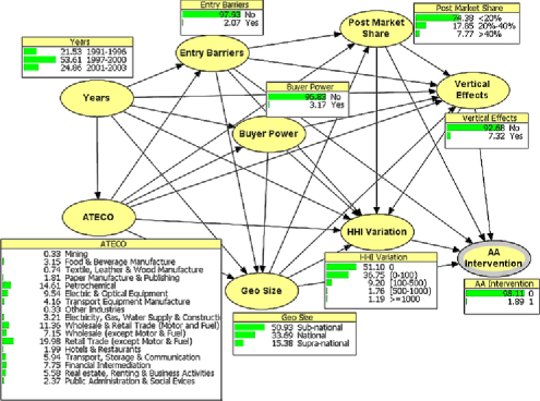
The dependence structure—based on the logical constraints given in Figure 2—learnt from the data is shown in Figure 3. The main dependence relationships estimated from the data are as follows: [(iii)]

The market of interest (ATECO) can depend on Year: an economic sector could be more relevant and worth investigating during one of the three reference periods (note that the president of the AA changed in 1997 and from 2001 Italian currency Lira was replaced by the Euro).

AA Intervention depends directly on HHI Variation, Vertical Effects, Post Market Share, Geo Size and Entry Barriers. Furthermore, the relevant market (ATECO) does not affect AAs decision (AA Intervention) directly but only through the relevant features of the market and of the merging firms (HHI Variation, Vertical Effects, Post Market Share, Geo Size and Entry Barriers).

These results are consistent with those in Bergman, Jakobsson and Razo (2005) and La Noce et al. (2006).

The Herfindahl–Hirschman concentration index variation (HHIVariation) depends on all the variables that logically precede it or are on an equal footing (as shown in Figure 2), whereas Post Market Share depends only on Entry Barriers, Geo Size and ATECO. An explanation of this could be that when a market sector is characterised by entry barriers (because of patents or increasing returns to scale) we expect that this market may be composed of a few firms with high market shares, thus influencing Post Market Share and a relevant HHI Variation. Many other conditional independencies can be read off the AA network in Figure 3, but for brevity they will not be presented here.

3.3 Estimation of the probability tables

To complete the construction of our model, we estimate the conditional probability distributions of the variables from the data. The EM-algorithm [Dempster, Laird and Rubin (1977)] is used for learning the probabilities.

The network in Figure 3 exhibits a complex association structure among the variables. For example, node HHI variation has seven parents. Its conditional probability table has $17\times 3^{3}\times 2^{3}\times 5=18\mbox{,}360$ entries corresponding to the state space of its parent variables: ATECO, Post Market Share, Years, Geo Size, Entry Barriers, Buyer Power, Vertical Effects, as well as HHI Variation’s state space. Many of these combinations are not represented in the data set, although they cannot be considered impossible ex ante. In fact, according to Bergman, Jakobsson and Razo (2005), if a threshold for relevant variables—like post market share—can be detected in AAs legal practice, this threshold may vary according to other variables, such as buyer power and entry barriers. Therefore, no variable level combinations can in principle be ruled out. So, in order to avoid that certain possible configurations in the conditional probability tables have zero probability, we set noninformative nonzero prior probabilities.

Figure 3 displays the marginal probabilities estimated from our data. Note, for example, that the probability of an AA intervention is only $0.0189$, which could be due to the fact that in most cases, $74.38\%$, the post market share is less than $20\%$ and entry barriers and vertical effects are absent (with probability $0.9793$ and $0.9268$, resp.), HHI index is less than 100 in $87.85\%$ of the cases and only in $15.38\%$ the geographical size is supra-national.

3.4 Using the network

Once the model has been estimated, we can address a number of questions about the AAs decision process. Various possible scenarios can be examined by inserting and propagating the appropriate evidence throughout the network. We illustrate three hypothetical scenarios.

Scenario A. What is the probability of an AA intervention in a merger request when there are entry barriers in the market? This scenario is represented in Figure 4(a). The posterior probability of an AA Intervention increases from $0.0189$ to $0.5790$ when the evidence Entry Barriers${}={}$Yes is inserted and propagated throughout the network.

Figure 4: Scenarios (a), (b) and (c) giving marginal posterior probabilities for the AA network.

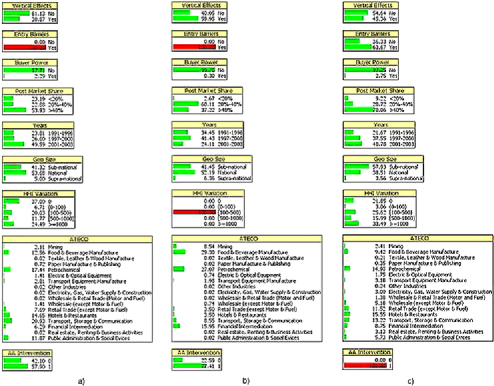
Scenario B. How would the probability obtained in Scenario A change if the Herfindahl–Hirschman concentration index variation (HHI variation) is in the class $[100,500)$? Note in Figure 4(b) that the probability of AA Intervention now increases to $0.7741$.

The network can be used not only for direct reasoning about the probability of AA Intervention, but also for reasoning about possible “causes” of a given AA decision.

Scenario C. A question about competition authorities’ behaviour that has been rarely addressed in the literature is about the type of mergers that are typically prohibited [Bergman, Jakobsson and Razo (2005)]. Our network can be used for this purpose. Suppose that the AA decides to intervene in a firm’s merger request. What are the most plausible reasons of this decision? Figure 4(c) gives the posterior probabilities given the evidence that AA Intervention is equal to one. On comparing Figures 3 and 4(c) we see that:

• The probability of entry barriers increases from 0.0207 to 0.6367;

• The probability of vertical effects increases from 0.0732 to 0.4536. This is an interesting result, since, although there is common agreement about the relevance of vertical effects for AAs decision on a merger request, it is controversial whether vertical effects influence the market negatively by foreclosing competitors or positively by reducing transaction costs. Here we find that the presence of vertical effects is much more probable for those firms where AA decides to intervene. La Noce et al. (2006) found similar results.

• The probability of post market share less than $20\%$ decreases from 0.7438 to 0.0922, whereas the probability of post market share greater than $40\%$ increases from 0.0777 to 0.7006.

• The HHI index decreases in the first two classes and increases in the last three classes.

Note that when evidence is propagated in the network, all marginal probability tables are updated accordingly.

=125pt Firm2 $C$ $D$ Firm1 $C$ $a,a$ $c,d$ $D$ $d,c$ $b,b$

Table 2: Payoff matrix for the prisoner’s dilemma

4 Duopoly representation

4.1 The prisoner’s dilemma

The prisoner’s dilemma [Flood (1958)] describes cooperation by rational agents. The PD is a 2-player symmetric game where the two players have the same rôle and have the same set of potential strategies termed cooperate $C$ and defect $D$. The PD is a simultaneous game where the players choose just once and simultaneously and the unique equilibrium is the pair of strategies ($D$, $D$). Players’ payoffs are such that defect is a dominant strategy, that is, a strategy that is preferred by each player independently of his/her rival. The problem is that this strategy is inefficient since both players would gain more if they cooperated and adopted the ($C$, $C$) strategy. The source of the dilemma lies in the fact that each player has an incentive to defect if the rival player cooperates, so that an agreement to cooperate would not be credible.

Simultaneous games, such as the PD, are commonly represented in either the normal or the extensive form. In the normal form representation, the PD can be described by the payoff matrix in Table 2. The two firms, Firm1 and Firm2, have two available strategies: cooperate $C$ or defect $D$. The payoffs need to be such that $d>a>b\geq c$ and $2a>(c+d)>2b$, so that $(C,C)$ maximises players’ joint payoff. Given that $b<a$, the strategy pair $(D,D)$ is strictly worse than $(C,C)$.

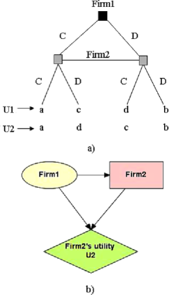
In the extensive form the game is represented by a tree. Figure 5(a) shows the tree representation (equivalent to Table 2) of the simultaneous duopoly game. Firm1 moves first and chooses either $C$ or $D$, Firm2 moves second but without knowing what Firm1 did.

Figure 5: (a) Tree representation of the simultaneous duopoly game. (b) Corresponding Bayesian network representation.

A symmetric duopoly, such as a market with two symmetric profit-maximising firms in mutual competition, can be modelled as a PD. The duopoly profit is the gain of each of the sellers in this market.

Suppose the two firms produce identical goods, incurring constant marginal costs, and they compete setting their prices. Since consumers will buy from the firm charging the lowest price, firms have an incentive to undercut their price to conquer the market (noncooperative or defect strategy). At equilibrium firms will set the competitive price (the market price under perfect competition which is equal to firm’s marginal cost of production), gaining duopoly profit $b=0$. This result is often called a paradox, since there are just two firms in the market and still the perfectly competitive strategy yields zero profit. However, if firms decide to cooperate and set the monopoly price, they can share positive monopoly profits. The monopoly profit is always greater than twice the duopoly profit, $2a>2b$.

In most markets, from a consumer’s point of view, goods are not identical. This gives firms the ability to raise the price above the marginal cost of production without losing their customers to competitors. In a symmetric duopoly with product differentiation firms produce and sell differentiated goods (imperfect substitutes). As long as product differentiation is not too large, firms face a PD: if they cooperate, they could share monopoly profit, but they have incentive to defect if the rival cooperates. However, when goods are imperfect substitutes, firms make positive duopoly profit, $b>0$, under the noncooperative strategy pair $(D,D)$. This duopoly profit is smaller than half the monopoly profit, $b<a$, so that the cooperative strategy $C$ is superior for each firm singly.

4.2 The prisoner’s dilemma network

Bayesian networks for decision support systems can incorporate both decision nodes and utility nodes [Jensen (2001)], giving rise to an influence diagram (ID) representation. IDs were extended by Lauritzen and Nilsson (2001) to allow for limited information decision problems (LIMIDs). A different approach to represent and solve games using graphical models was initially proposed by Smith (1996) and later by La Mura (2000), Kearns, Littman and Singh (2001) and Koller and Milch (2003).

The one stage PD being a symmetric game can be represented by the ID network in Figure 5(b). The simultaneity of the game is implemented by representing Firm1 as a random variable (oval node) and Firm2 as the decision maker (rectangular node) having two possible actions: defect $D$ and cooperate $C$. Firm2’s decision is influenced by Firm1. Firm1’s associated prior probability distribution represents Firm2’s subjective opinion about Firm1’s behaviour. Random variable Firm1 has two states, defect (coded as 0) and cooperate (coded as 1), with uniform prior probabilities indicating Firm2’s ignorance about Firm1’s choice. Firm2 could assign different prior probabilities based on his/her prior knowledge about Firm1’s behaviour. Table 3 shows Firms2’s utility [node Firm2’s utility U2 in Figure 5(b)] based on Firm1 and Firm2’s actions. Thanks to game symmetry, Table 3 is equivalent to the normal form payoff matrix given in Table 2.

=275pt Firm1 Defect (0) Cooperate (1) Firm2 Defect (0) Cooperate (1) Defect (0) Cooperate (1) U2 $b$ $c$ $d$ $a$

Table 3: Firm2’s utility U2 conditional on Firm1 and Firm2’s actions

Once the network is compiled, the optimal decision for Firm2 is automatically computed by maximising expected utility. Since the game is symmetric, Firm2’s optimal strategy coincides with Firm1’s optimal strategy and this pair of strategies constitutes a Nash equilibrium. Thus, in the ID representation the choice of Firm2 as decision maker is without loss of generality.

In what follows we always consider Firm2 as the decision maker. The prior probability distribution on the random variable Firm1 reflects Firm2’s subjective opinion on the type of rival player he/she is playing against.

4.3 Repeated prisoner’s dilemma

Since firms interact more than once, we need to consider the repeated version of the PD. In repeated games, players’ actions are observed at the end of each period and their overall payoff is the sum of the payoffs in each stage discounted by a factor $\delta\in[0,1]$. Thus, players may condition their play on the opponents past play. Here we assume that firms never forget previous moves and other information acquired, in other words, we assume that firms have perfect recall.

The repeated PD analyzes how threats and promises about future behaviour can affect and improve current behaviour. When the time horizon is indefinite firms may decide to adopt a cooperative strategy where the discount factor $\delta$ represents uncertainty about the number of stages faced by firms. This uncertainty is usually not modelled within the game itself. In Section 5 we illustrate how to incorporate this uncertainty in the merger control problem.

4.4 OOBN for repeated prisoner’s dilemma

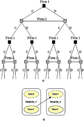
Generalising the tree representation in Figure 5(a) to repeated games is both computationally and graphically demanding. The game tree grows exponentially with the number of stages. For example, Figure 6(a) shows the tree representation of a two-stage PD.

Figure 6: (a) Tree representation of the two-stage duopoly game. (b) Corresponding OOBN representation.

OOBNs are particularly well suited for an application area such as the present because the similarity between network elements (the stages of the game) can be exploited in a modular and flexible construction. Object-oriented Bayesian networks have a hierarchical structure where a node itself can represent a (object-oriented) network containing several instances of other generic classes of networks. Instances have interface input and output nodes as well as ordinary nodes. Instances of a particular class have identical conditional probability tables for noninput nodes. Instances are connected by arrows from output nodes into input nodes. These arrows, as well as those from ordinary nodes to input nodes, represent identity links, whereas arrows between two ordinary nodes or an output node and an ordinary node represent probabilistic dependence. The graphical simplicity automatically produces computational efficiency. As a result, increasingly complex networks can be constructed by simply adding new objects which perform different tasks.

Since we assume perfect recall, Hugin version 6.9 software, which automatically implements the fact that at every stage the decision maker recalls all previous decisions, is used to build the networks. This implies that each decision depends on the decisions taken in all previous stages, so even though the graphical representation does not implicitly represent this, in the junction tree construction [Cowell et al. (1999)] these dependencies are explicitly considered. In what follows we indicate an instance in bold. Figure 6(b) shows the OOBN two-stage repeated game that corresponds to the tree representation in Figure 6(a). Each rounded rectangle represents an instance termed Duopoly and models a stage of the repeated game. In order to specify the links between successive stages (instances), Figure 5(b) (which represents each Duopoly instance) needs to be generalised as shown in Figure 7.

Figure 7: Class network for repeated PD with associated marginal prior probability tables.

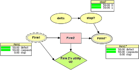
=290pt Stop? No (0) Yes (1) Firm2 Defect (0) Cooperate (1) Defect (0) Cooperate (1) Defect (0) 1 0 0 0 Cooperate (1) 0 1 0 0 Stop (2) 0 0 1 1

Table 4: Conditional probability table for Firm1^∗ given stop? and Firm2

The node Firm1^∗ models the behaviour of Firm1 in the next stage. In each stage the game can either continue or terminate. Firm1 and Firm1^∗ now need to be given three states: defect (0), cooperate (1) and stop (2). Since in a repeated game every stage depends on the actions taken in the previous stages, Firm1^∗ is logically dependent on Firm2. Uncertainty about the existence of further stages is modelled by adding a new random node stop?. Node stop? has two states, $\{0,1\}$ according to whether the game continues or stops and has a Bernoulli distribution $\operatorname{Bin}(1,1-\mbox{{delta}})$. The parameter node delta is the probability that the game continues $P(\mbox{{stop?}}=0)$. Node delta has a uniform prior distribution over a plausible set of values.

In the first stage, to ensure that the game starts, Firm1 can only choose between defect and cooperate. Table 4 gives the conditional probability distribution of Firm1^∗ given stop? and Firm2. It shows that if the game stops (stop?${}={}$1), Firm1^∗ stops with certainty, else Firm1^∗ cooperates or defects according to Firm2’s decision. This implements the tit for tat (TFT) strategy in which Firm1 begins by cooperating and cooperates as long as Firm2 cooperates, and defects otherwise. Variations on this strategy will be shown in Section 4.4.1.

4.4.1 Other strategies

Experimental results show that people, contrary to standard prescriptions of game theory, may cooperate more frequently than expected [Andreoni and Miller (1993)]. An explanation behind this empirical evidence is provided by the theoretical models of Kreps and Wilson (1982) and Kreps et al. (1982). Figure 7 can be modified to provide a general class network that explicitly incorporates a set of potential strategies for Firm1 other than TFT. This network is displayed in Figure 8. The network can, for example, model a repeated PD with incomplete information, that is, where there is uncertainty about the type of rival that a firm is going to face. The conditional probability distribution of Firm1^∗ reflects Firm2’s uncertainty about its opponent. If Firm2 believes Firm1 to be “altruistic”, it can expect Firm1 to cooperate, with probability $\alpha_{D}>0$, even if it defected in the previous stage. On the other hand, if Firm2 believes Firm1 to be “egoistic”, then it expects Firm1 to cooperate, with probability $\alpha_{C}<1$, even if it cooperated in the previous stage.

Figure 8: Generalised repeated PD network representing various strategies and incomplete information.

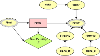
Additional nodes, Firm1^∗|D and Firm1^∗|C, having Bernoulli distributions with parameter nodes alpha_D and alpha_C are added to the network of Figure 7. Node Firm1^∗ takes value 2 if the game stops in the current stage, whereas if the game continues (stop?${}={}$0), the value of Firm1^∗ depends on that of Firm2. If Firm2 defects (cooperates), Firm1^∗ is Firm1^∗|D (Firm1^∗|C), with alpha_D (alpha_C) being the probability that Firm1 will cooperate in the next stage given that Firm2 defected (cooperated) in the previous stage. The conditional probability distribution of Firm1^∗ is thus defined by the logical expression $\mbox{{if}}(\mbox{{stop}}==1,2,\mbox{{if}}(\mbox{{Firm2}}==0,\mbox{{Firm1${}^{*}$|D}},\break\mbox{{Firm1${}^{*}$|C}}))$. Firm1^∗ represents Firm2’s subjective opinions about Firm1’s behaviour in each single stage of the repeated game.

This model can also incorporate a large set of strategies, including TFT, and it can model scenarios where the probability that the game continues depends on external factors. An illustrative example is given in Section 5.

Figure 9: Integrated AA-duopoly merger stage game.

5 Global network

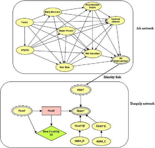
Thanks to the modularity and flexibility of OOBNs, it is possible to integrate the AA and the Duopoly networks, giving rise to a unique overall OOBN representation of the problem [Figure 1(a)]. An expanded representation of this model is shown in Figure 9.

The Duopoly network (the bottom network) in Figure 9 is similar to the network in Figure 8 except that the uncertainty about the next stage stop? is now identified with AA Intervention in the AA network (the top network in Figure 9) representing AAs decision process.

The AA decision process is usually dynamic; it can change over time due to changes in the antitrust law as well as changes in market conditions. We are thus interested in the repeated version of the model in Figure 9.

Figure 10: OOBN representing a three-stage repeated merger game with uncertainty about the number of stages.

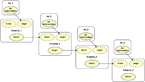
Figure 10 represents the global model (Figure 9) repeated four times for a three-stage merger game with uncertainty on the number of stages. In general, an OOBN with $n+1$ instances models a game repeated $n$ times with uncertainty about the successive stage. In this model, the AAs decision process is represented by the same instance in each period. This is justified by assuming that, even if the AA decides not to intervene, it continues monitoring firms’ behaviour in successive stages.

5.1 Firms’ strategy

We now study the sensitivity of cooperative behaviour with respect to two sets of utilities and all the factors that might directly or indirectly influence the AAs decision. We consider both the TFT strategy and a more general strategy. The TFT strategy can be implemented using the global network by setting Firm1${}^{*}=1$ in stage Duopoly_1 and Firm1^∗|C${}={}$1, Firm1^∗|D${}={}$0 in all other stages.

5.1.1 TFT strategy: Perfect substitutability

Table 5 shows an example of Firm2’s utility for a market with perfect substitutable goods. Figures 11, 12 and 13 show the marginal probabilities for a selection of random variables and the expected utilities for the decision nodes in the first stage AA_1 and Duopoly_1.

=270pt Firm1 Defect (0) Cooperate (1) Firm2 Defect (0) Cooperate (1) Defect (0) Cooperate (1) U2 0 $-$10 150 100

Table 5: Firm2’s utility U2 for a market with perfect substitutability

Figure 11: Marginal probabilities and optimal decision in the first stage AA_1 and Duopoly_1, under perfect substitutability, when Firm1 plays TFT.

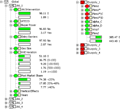
When no evidence about the variables in the market is inserted in the network (Figure 11) Firm2’s optimal decision is to cooperate (1), having expected utility equal to 443.40 (while defect has expected utility equal to 385.47). This could be in part due to the small probability of an AA intervention, 0.0189.

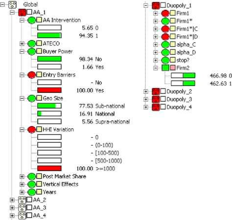
Figure 12 shows the case where there are entry barriers in the market of interest (Entry Barriers${}={}$Yes) and the merger causes the HHI variation to be in the last class (HHI Variation${}>={}$1000). The resulting probability of AA intervention shoots up to 0.9435 and Firm2’s optimal decision is to defect with expected utility of 394.72, against 350.93 for cooperating. This strategy still remains optimal (although with a smaller gap between the expected utilities) when based only on the presence of entry barriers.

Figure 12: Marginal probabilities and optimal decision in the first stage AA_1 and Duopoly_1, under perfect substitutability, when Firm1 plays TFT, Entry Barriers${}={}$Yes and HHI Variation${}>={}$1000.

Figure 13: Marginal probabilities and optimal decision in the first stage AA_1 and Duopoly_1, under perfect substitutability, when Firm1 plays TFT, Entry Barriers${}={}$Yes, HHI Variation${}>={}$1000 and Buyer Power${}={}$Yes.

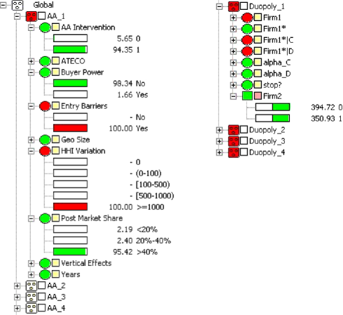
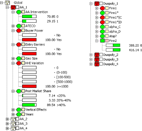
Figure 13 shows the case where, as before, there are entry barriers, the HHI variation is $\geq$1000, and customers exert competitive pressure on the merging parties (Buyer Power${}={}$Yes). The probability of AA intervention decreases from 0.9435 to 0.2915 and Firm2’s optimal decision is to cooperate, having expected utility of 416.14. It is interesting to note that buyer power is able to counterbalance the effect of both entry barriers and a large HHI variation.

5.1.2 TFT strategy: Imperfect substitutability

We now use Firm2’s utility for a market with imperfect substitutable goods given in Table 6.

Figure 14 shows results when evidence about the market is not available. Firm2’s optimal decision is to cooperate (1), having expected utility equal to 601.33 (while defect has expected utility equal to 513.21). Again, this is most plausibly due to the small probability of an AA intervention.

When Entry Barriers${}={}$Yes and HHI Variation${}>={}$1000, Firm2’s expected utility to cooperate or to defect is almost equal, although the probability of AA intervention is close to 1 (Figure 15).

=270pt Firm1 Defect Cooperate Firm2 Defect Cooperate Defect Cooperate U2 100 50 160 150

Table 6: Firm2’s utility U2 for a market with imperfect substitutability

Figure 14: Marginal probabilities and optimal decision in the first stage AA_1 and Duopoly_1, under imperfect substitutability, when Firm1 plays TFT.

Figure 15: Marginal probabilities and optimal decision in the first stage AA_1 and Duopoly_1, under imperfect substitutability, when Firm1 plays TFT, Entry Barriers${}={}$Yes and HHI Variation${}>={}$1000.

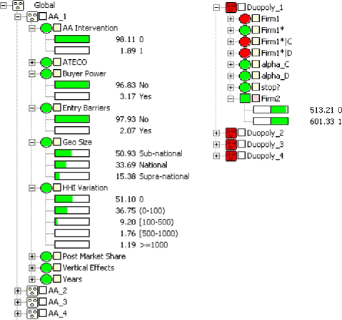
Furthermore, in contrast to perfect substitutability, accounting for the presence of entry barriers alone is not sufficient to modify the optimal decision from cooperate to defect. The main reason being that when the firms’ products are imperfect substitutes, the set of utilities reflects the fact that the defect strategy does not correspond to such a strong punishment, so that a firm can continue to cooperate even if there is high risk that the game might stop.

5.1.3 Incomplete information

Assume that Firm2 has incomplete information about the type of rival it is going to face. This is a reasonable scenario, as firms are likely to be uncertain about their rivals’ costs and benefits from cooperation.

Table 7: Firm2’s expected utility for different values of $\alpha_{C}$ and $\alpha_{D}$, without evidence, with evidence $E_{1}$ and $E_{2}$, for likelihood evidence and for the TFT strategy

		Without evidence		With evidence $\bolds{E_{1}}$		With evidence $\bolds{E_{2}}$
$\bolds{\alpha_{C}}$	$\bolds{\alpha_{D}}$	$\bolds{\mathbb{E}[u(D)]}$	$\bolds{\mathbb{E}[u(C)]}$	$\bolds{\mathbb{E}[u(D)|E_{1}]}$	$\bolds{\mathbb{E}[u(C)|E_{1}]}$	$\bolds{\mathbb{E}[u(D)|E_{2}]}$	$\bolds{\mathbb{E}[u(C)|E_{2}]}$
1	$0.25$	337	388	329	339	322	298
0.8	$0.25$	286	316	278	277	271	245
0.6	$0.25$	238	250	228	219	220	193
0.4	$0.25$	203	193	190	170	180	152
1	$0.2$	332	388	326	339	321	298
0.8	$0.2$	281	316	275	277	270	245
0.6	$0.2$	231	247	225	217	219	193
0.4	$0.2$	192	188	183	167	177	149
1	$0.1$	321	388	321	339	320	298
0.8	$0.1$	270	316	270	277	269	245
0.6	$0.1$	219	243	219	215	218	193
0.4	$0.1$	172	179	171	159	170	143
Likelihood		280	313	273	275	268	243
TFT		385	443	390	394	395	353

Table 7 shows Firm2’s expected utility in case of perfect substitutability (based on Firm2’s utility given in Table 5) for different probability values of $\alpha_{C}$ and $\alpha_{D}$ (nodes alpha_C and alpha_D in Figure 9). Three types of information about the relevant market are considered: no evidence, evidence $E_{1}=\{\mbox{{Post} {Market} {Share}}\geq 40\%$, Entry Barriers${}={}$Yes and Buyer Power${}={}$Yes} and evidence $E_{2}$${}={}${Entry Barriers${}={}$Yes and HHI Variation${}\in{}$[500–1000]}. The optimal decision yielding the highest expected utility for each scenario is italicised.

The second last row of Table 7 gives the results when inserting a uniform likelihood function for $\alpha_{C}>0.5$ and $\alpha_{D}<0.5$. In this case, Firm2’s optimal decision is to cooperate under no evidence and $E_{1}$. Whereas, for $E_{2}$, when the probability of AA intervention is close to one, $\mathbb{E}[u(D)|E_{2}]>\mathbb{E}[u(C)|E_{2}]$, so Firm2’s optimal decision is to defect. These results coincide with those obtained using the TFT strategy shown in the last row of Table 7. Recall that the TFT strategy corresponds to setting $\alpha_{C}=1$ and $\alpha_{D}=0$ in all Duopoly instances.

Now, suppose Firm2 believes that its rival cooperates—with probability $\alpha_{C}=0.8$—if Firm2 cooperates; and cooperates—with probability $\alpha_{D}=0.25$—even if Firm2 defects. This is implemented in the network inserting and propagating evidence alpha_C${}={}$0.8 and alpha_D${}={}$0.25 in each Duopoly instance. As we can see in Table 7, Firm2’s expected utility to cooperate, $\mathbb{E}[u(C)]=316$, is greater than to defect, $\mathbb{E}[u(D)]=286$. Introducing evidence $E_{1}$ in AA_1, the two decisions become almost utility equivalent. Whereas, under the TFT strategy, $E_{1}$ yields an optimal decision to cooperate $\mathbb{E}[u(C)|E_{1}]=394$, whereas $\mathbb{E}[u(D)|E_{1}]=390$.

Recall that when information about the relevant market is not taken into account, the probability of AA intervention is 0.0189. If the probability that Firm1 cooperates when Firm2 defects is very small ($\alpha_{D}=0.1$), then its optimal decision is to cooperate, even for small values of $\alpha_{C}$. On the other hand, when $\alpha_{D}\geq 0.2$, defecting is Firm2’s best choice for $\alpha_{C}=0.4$, yielding a different behaviour from that obtained using the TFT strategy. However, using evidence $E_{1}$, when the probability of AA intervention is 0.514, $\mathbb{E}[u(D)|E_{1}]>\mathbb{E}[u(C)|E_{1}]$ even when Firm1 is slightly altruistic, $\alpha_{D}\leq 0.2$ and $\alpha_{C}\leq 0.6$. Furthermore, if $\alpha_{D}=0.25$, then $\mathbb{E}[u(D)|E_{1}]>\mathbb{E}[u(C)|E_{1}]$ also for $\alpha_{C}\leq 0.8$. If the TFT strategy is adopted, Firm2 optimally cooperates both under no evidence and $E_{1}$, whereas for $E_{2}$ the associated probability of AA intervention is very large, so that Firm2’s optimal decision is to defect for all values of $\alpha_{C}$ and $\alpha_{D}$ considered here.

While the examples shown here are merely illustrative, the number of questions and different strategies that can be analysed is clearly huge and increases with the number of stages considered.

6 Conclusion

When the antitrust authority starts an investigation, the two potentially merging firms are likely to represent a relevant share of the market, hence, they might affect the price of the goods traded. In contrast, the decisions of other firms inside the market, but outside the merged entity, can be assumed to be irrelevant. In circumstances such as these, a PD duopoly model is a reasonable representation.

From an economic perspective, the methodology we present can be seen as a useful decision support system. It models and integrates the different uncertainty sources deriving from a rival competitor and from the economic environment. Furthermore, the model can be updated as we consider new cases, changes in market conditions or new antitrust regulations. The emphasis in this paper is to show the potentiality of OOBNs in the analysis of duopoly markets with external uncertainty. For the sake of simplicity, the duopoly is represented by a rather naive game theoretic model; in future studies we wish to implement a more complex interaction model between firms.

As is standard in industrial organization, the firm is seen as a single decision making unit; generalisations of our OOBN to model firms’ internal organization could also be considered. Indeed, a firm’s top and middle management may have different objectives from its owner. An appropriate BN could be built to model these interrelationships and incorporate them into a more general OOBN model. This would yield a more complete and realistic picture of firms’ cooperative behaviour. We hope to develop this and other aspects in the future.

References

- Andreoni and Miller (1993) {barticle}[auto:STB—2013/04/11—08:11:48] \bauthor\bsnmAndreoni, \bfnmJ.\binitsJ. and \bauthor\bsnmMiller, \bfnmJ.\binitsJ. (\byear1993). \btitleRational cooperation in the finitely repeated prisoner’s dilemma: Experimental evidence. \bjournalEconomic Journal \bvolume103 \bpages570–585. \bptokimsref \endbibitem
- Bangsø and Wuillemin (2000) {bmisc}[auto:STB—2013/04/11—08:11:48] \bauthor\bsnmBangsø, \bfnmO.\binitsO. and \bauthor\bsnmWuillemin, \bfnmP.\binitsP. (\byear2000). \bhowpublishedObject oriented Bayesian networks: A framework for topdown specification of large Bayesian networks and repetitive structures. Technical report, Dept. Computer Science, Aalborg Univ. \bptokimsref \endbibitem
- Bergman, Jakobsson and Razo (2005) {barticle}[auto:STB—2013/04/11—08:11:48] \bauthor\bsnmBergman, \bfnmM. A.\binitsM. A., \bauthor\bsnmJakobsson, \bfnmM.\binitsM. and \bauthor\bsnmRazo, \bfnmC.\binitsC. (\byear2005). \btitleAn econometric analysis of the European Commissions merger decisions. \bjournalInternational Journal of Industrial Organization \bvolume23 \bpages717–737. \bptokimsref \endbibitem
- Cowell et al. (1999) {bbook}[mr] \bauthor\bsnmCowell, \bfnmRobert G.\binitsR. G., \bauthor\bsnmDawid, \bfnmA. Philip\binitsA. P., \bauthor\bsnmLauritzen, \bfnmSteffen L.\binitsS. L. and \bauthor\bsnmSpiegelhalter, \bfnmDavid J.\binitsD. J. (\byear1999). \btitleProbabilistic Networks and Expert Systems. \bpublisherSpringer, \blocationNew York. \bidmr=1697175 \bptokimsref \endbibitem
- Dempster, Laird and Rubin (1977) {barticle}[mr] \bauthor\bsnmDempster, \bfnmA. P.\binitsA. P., \bauthor\bsnmLaird, \bfnmN. M.\binitsN. M. and \bauthor\bsnmRubin, \bfnmD. B.\binitsD. B. (\byear1977). \btitleMaximum likelihood from incomplete data via the EM algorithm. \bjournalJ. R. Stat. Soc. Ser. B Stat. Methodol. \bvolume39 \bpages1–38. \bidissn=0035-9246, mr=0501537 \bptnotecheck related\bptokimsref \endbibitem
- Flood (1958) {barticle}[mr] \bauthor\bsnmFlood, \bfnmMerrill M.\binitsM. M. (\byear1958). \btitleSome experimental games. \bjournalManagement Sci. \bvolume5 \bpages5–26. \bidissn=0025-1909, mr=0097986 \bptokimsref \endbibitem
- Jensen (2001) {bbook}[mr] \bauthor\bsnmJensen, \bfnmFinn V.\binitsF. V. (\byear2001). \btitleBayesian Networks and Decision Graphs. \bpublisherSpringer, \blocationNew York. \bidmr=1876880 \bptokimsref \endbibitem
- Kearns, Littman and Singh (2001) {bincollection}[auto:STB—2013/04/11—08:11:48] \bauthor\bsnmKearns, \bfnmM.\binitsM., \bauthor\bsnmLittman, \bfnmM.\binitsM. and \bauthor\bsnmSingh, \bfnmS.\binitsS. (\byear2001). \btitleGraphical models for game theory. In \bbooktitleProceedings of the 17th Conference in Uncertainty in Artificial Intelligence \bpages253–260. \bpublisherMorgan Kaufmann, \blocationSan Francisco, CA. \bptokimsref \endbibitem
- Koller and Milch (2003) {barticle}[mr] \bauthor\bsnmKoller, \bfnmDaphne\binitsD. and \bauthor\bsnmMilch, \bfnmBrian\binitsB. (\byear2003). \btitleMulti-agent influence diagrams for representing and solving games. \bjournalGames Econom. Behav. \bvolume45 \bpages181–221. \biddoi=10.1016/S0899-8256(02)00544-4, issn=0899-8256, mr=2022867 \bptokimsref \endbibitem
- Koller and Pfeffer (1997) {bincollection}[auto:STB—2013/04/11—08:11:48] \bauthor\bsnmKoller, \bfnmD.\binitsD. and \bauthor\bsnmPfeffer, \bfnmA.\binitsA. (\byear1997). \btitleObject-oriented Bayesian networks. In \bbooktitleProceedings of the 13th Annual Conference on Uncertainty in AI (UAI) \bpages302–313. \bpublisherMorgan Kaufmann, \blocationSan Francisco, CA. \bptokimsref \endbibitem
- Kreps and Wilson (1982) {barticle}[mr] \bauthor\bsnmKreps, \bfnmDavid M.\binitsD. M. and \bauthor\bsnmWilson, \bfnmRobert\binitsR. (\byear1982). \btitleReputation and imperfect information. \bjournalJ. Econom. Theory \bvolume27 \bpages253–279. \biddoi=10.1016/0022-0531(82)90030-8, issn=0022-0531, mr=0671658 \bptokimsref \endbibitem
- Kreps et al. (1982) {barticle}[mr] \bauthor\bsnmKreps, \bfnmDavid M.\binitsD. M., \bauthor\bsnmMilgrom, \bfnmPaul\binitsP., \bauthor\bsnmRoberts, \bfnmJohn\binitsJ. and \bauthor\bsnmWilson, \bfnmRobert\binitsR. (\byear1982). \btitleRational cooperation in the finitely repeated prisoners’ dilemma. \bjournalJ. Econom. Theory \bvolume27 \bpages245–252. \biddoi=10.1016/0022-0531(82)90029-1, issn=0022-0531, mr=0671657 \bptokimsref \endbibitem
- La Mura (2000) {bincollection}[auto:STB—2013/04/11—08:11:48] \bauthor\bsnmLa Mura, \bfnmP.\binitsP. (\byear2000). \btitleGame networks. In \bbooktitleIn Proceedings of the 16th Conference on Uncertainty in Artificial Intelligence (UAI) \bpages335–342. \bpublisherMorgan Kaufmann, \blocationSan Francisco, CA. \bptokimsref \endbibitem
- La Noce et al. (2006) {barticle}[auto:STB—2013/04/11—08:11:48] \bauthor\bsnmLa Noce, \bfnmM.\binitsM., \bauthor\bsnmBolasco, \bfnmS.\binitsS., \bauthor\bsnmAllegra, \bfnmE.\binitsE., \bauthor\bsnmRuocco, \bfnmV.\binitsV. and \bauthor\bsnmCapo, \bfnmF. M.\binitsF. M. (\byear2006). \btitleMerger control in Italy 1995–2003: A statistical study of the enforcement practice by mining the text of Authority resolutions. \bjournalInternational Journal of the Economics of Business \bvolume13 \bpages307–334. \bptokimsref \endbibitem
- Lauritzen and Nilsson (2001) {barticle}[auto:STB—2013/04/11—08:11:48] \bauthor\bsnmLauritzen, \bfnmS. L.\binitsS. L. and \bauthor\bsnmNilsson, \bfnmD.\binitsD. (\byear2001). \btitleRepresenting and solving decision problems with limited information. \bjournalManagement Sci. \bvolume47 \bpages1238–1251. \bptokimsref \endbibitem
- Smith (1996) {bincollection}[mr] \bauthor\bsnmSmith, \bfnmJ. Q.\binitsJ. Q. (\byear1996). \btitlePlausible Bayesian games. In \bbooktitleBayesian Statistics, 5 (Alicante, 1994) (\beditorJ. M. Bernardo, \beditorJ. O. Berger, \beditorA. P. Dawid and \beditorA. F. M. Smith, eds.) \bpages387–405. \bpublisherOxford Univ. Press, \blocationNew York. \bidmr=1425416 \bptokimsref \endbibitem
- Steck (2001) {bmisc}[auto:STB—2013/04/11—08:11:48] \bauthor\bsnmSteck, \bfnmH.\binitsH. (\byear2001). \bhowpublishedConstraint-based structural learning in Bayesian networks using finite data sets. Ph.D. thesis, Dept. Computer Science, Univ. Munich. \bptokimsref \endbibitem
- Young and Smith (1992) {barticle}[mr] \bauthor\bsnmYoung, \bfnmS. C.\binitsS. C. and \bauthor\bsnmSmith, \bfnmJ. Q.\binitsJ. Q. (\byear1992). \btitleSuboptimality of -step back strategies in Bayesian games. \bjournalInternat. J. Game Theory \bvolume21 \bpages57–74. \biddoi=10.1007/BF01240252, issn=0020-7276, mr=1178813 \bptokimsref \endbibitem