DYNAMO ACTIVITIES DRIVEN BY MAGNETO-ROTATIONAL INSTABILITY AND PARKER INSTABILITY IN GALACTIC GASEOUS DISK

Abstract

We carried out global three-dimensional magneto-hydrodynamic simulations of dynamo activities in galactic gaseous disks without assuming equatorial symmetry. Numerical results indicate the growth of azimuthal magnetic fields non-symmetric to the equatorial plane. As magneto-rotational instability (MRI) grows, the mean strength of magnetic fields is amplified until the magnetic pressure becomes as large as 10% of the gas pressure. When the local plasma $\beta$ ($=p_{\rm gas}/p_{\rm mag}$) becomes less than 5 near the disk surface, magnetic flux escapes from the disk by Parker instability within one rotation period of the disk. The buoyant escape of coherent magnetic fields drives dynamo activities by generating disk magnetic fields with opposite polarity to satisfy the magnetic flux conservation. The flotation of the azimuthal magnetic flux from the disk and the subsequent amplification of disk magnetic field by MRI drive quasi-periodic reversal of azimuthal magnetic fields in timescale of 10 rotation period. Since the rotation speed decreases with radius, the interval between the reversal of azimuthal magnetic fields increases with radius. The rotation measure computed from the numerical results shows symmetry corresponding to a dipole field.

1 Introduction

The origin and nature of magnetic fields in spiral galaxies is an open question. Magnetic fields in spiral galaxies have been intensively studied through observations of linear polarization of synchrotron radiation (Sofue, Fujimoto, & Wielebinski, 1986; Beck et al., 1996). The typical magnetic field strength is a few $\mu{\rm G}$ in the Milky Way near the Sun, and in spiral galaxies. The mean ratio of gas pressure to magnetic pressure is close to unity (Rand & Kulkarni, 1989; Crocker et al., 2010), suggesting that magnetic fields in spiral galaxies are strong enough to affect the motion of the interstellar matter in the gaseous disk.

Since the galactic gas disk rotates differentially, the magnetic field is amplified faster near the galactic center than in the outer disk, and the magnetic field strength can exceed $0.1{\rm mG}$ in the galactic center. An observational evidence of such strong magnetic fields has been obtained in the radio arc near the galactic center, where the field strength of about $1{\rm mG}$ is estimated from synchrotron radiation. Many threads perpendicular to the galactic plane are observed indicating strong vertical field (Yusef-Zadah, Morris, & Chance, 1984; Morris, 1990). On the other hand, observations of near infrared polarization suggested that horizontal fields of $0.1-1{\rm mG}$ are dominant inside the disk (Novak et al., 2000; Nishiyama et al., 2009).

Taylor, Stil, & Sunstrum (2009) presented results of all sky distribution of rotation measure (RM), which indicate that the magnetic fields along line-of-sights are roughly consistent with the dipole-like models in which the azimuthal magnetic fields are anti-symmetric with respect to the equatorial plane, rather than quadrupole-like models in which the azimuthal magnetic fields show symmetry with respect to the equatorial plane. They also showed that the RM distribution has small scale variations, which would be linked to turbulent structure of the gaseous disk. Han et al. (2002) showed a view of RM distributions from the North Galactic pole using the results of pulsar polarization measurements. They indicated that the magnetic field direction changes between the spiral arms (Han et al., 2002; Han & Zhang, 2007).

The magnetic fields have to be maintained for $10^{9}-10^{10}$ years, because most of spiral galaxies have magnetic fields with similar strength (Beck, 2012). Parker (1971) considered the self-sustaining mechanism of magnetic fields called the dynamo activity. In the framework of the kinematic dynamo, where the back-reaction by enhanced magnetic fields is ignored, Fujimoto & Sawa (1987) and Sawa & Fujimoto (1987) obtained the global structure of galactic magnetic fields. On the other hand, Balbus & Hawley (1991) pointed out importance of the magneto-rotational instability (MRI) in differentially rotating system, and showed that the back-reaction of the enhanced magnetic fields cannot be ignored. Since galactic gaseous disk is a differentially rotating system, magneto-rotational instability grows (Balbus & Hawley, 1991).

In this paper, we present the results of global three-dimensional magneto-hydrodynamic simulations of galactic gas disks assuming an axisymmetric gravitational potential and study the dynamo activities of the galactic gas disk.

In order to take into account the back reaction of magnetic fields on the dynamics of gas disk, we have to solve the magneto-hydrodynamic equations in which the induction equation is coupled with the equation of motion. This approach is called the dynamical dynamo. Nishikori, Machida & Matsumoto (2006) presented results of three dimensional magneto-hydrodynamic (MHD) simulations of galactic gaseous disks. They showed that, even when the initial magnetic field is weak, the dynamical dynamo amplifies the magnetic fields and can attain the current field strength observed in galaxies. They also showed that the direction of mean azimuthal magnetic fields reverses quasi-periodically, and pointed out that reversal of magnetic field is driven by the coupling of MRI and Parker instability. When the magnetic field is amplified by MRI, the time scale of buoyant escape of magnetic flux due to Parker instability becomes comparable to the growth time of MRI, and limits the strength of magnetic fields inside the disk.

Since Nishikori et al. (2006) assumed symmetric boundary condition at the equatorial plane of the disk, they could not simulate the growth of anti-symmetric mode of Parker instability, in which magnetic fields cross the equatorial plane (Horiuchi et al., 1988). The present paper is aimed at obtaining a realistic, quantitative model of the global magnetic field of the Milky Way Galaxy based on numerical 3D MHD simulations of magnetized galactic gaseous disk. In section 2, we show the initial setting of the simulation. We present the results of numerical simulations in section 3. The result will be used to compute the distribution of RM on the whole sky in section 4.

2 Numerical Models

2.1 Basic equations

We solved the resistive MHD equations by using modified Lax-Wendroff scheme with artificial viscosity (Rubin & Burstein 1967, Richtmyer & Morton 1967).

$$\frac{\partial\rho}{\partial t}+\nabla\cdot{\rho\mbox{\boldmath$v$}}=0$$ (1)

$$\frac{\partial\mbox{\boldmath$v$}}{\partial t}+(\mbox{\boldmath$v$}\cdot\nabla)\mbox{\boldmath$v$}=-\frac{1}{\rho}\nabla P-\nabla\phi+\frac{1}{4\pi\rho}(\nabla\times\mbox{\boldmath$B$})\times\mbox{\boldmath$B$}$$ (2)

$$\frac{\partial}{\partial t}\left(\frac{1}{2}\rho v^{2}+\frac{B^{2}}{8\pi}+\frac{P}{\gamma-1}\right)+\nabla\cdot\left[\left(\frac{1}{2}\rho\mbox{\boldmath$v$}^{2}+\frac{\gamma P}{\gamma-1}\right)\mbox{\boldmath$v$}+\frac{c}{4\pi}\mbox{\boldmath$E$}\times\mbox{\boldmath$B$}\right]=-\rho\mbox{\boldmath$v$}\nabla\phi$$ (3)

$$\frac{\partial\mbox{\boldmath$B$}}{\partial t}=\nabla\times(\mbox{\boldmath$v$}\times\mbox{\boldmath$B$}-\eta\nabla\times\mbox{\boldmath$B$})$$ (4)

where $\rho$, $P$, $v$, $B$, and $\gamma$ are the density, gas pressure, velocity, magnetic field, the specific heat ratio, respectively, and $\phi$ is gravitational potential proposed by Miyamoto & Nagai (1975). The electric field $E$ is related to magnetic field $B$ by Ohm’s law. We assume the anomolous resistivity $\eta$

$$\eta=\left\{\begin{array}[]{ll}\eta_{0}(v_{\rm d}/v_{\rm c}-1)^{2},&v_{\rm d}\geq v_{\rm c},\\ 0,&v_{\rm d}\leq v_{\rm c},\end{array}\right.$$ (5)

which sets in when the electron-ion drift speed $v_{\rm d}=j/\rho$, where $j$ is the current density, exceeds the critical velocity $v_{\rm c}$.

2.2 Simulation Setup

We assumed an equilibrium torus threaded by weak toroidal magnetic fields (Okada, Fukue & Matsumoto, 1989). The torus is embedded in a hot, non-rotating spherical corona. We assume that the torus has constant specific angular momentum $L$ at $\varpi=\varpi_{\rm b}$ and assume polytropic equation of state $P=K\rho^{\gamma}$, where $K$ is constant. The density distribution is same as that for equation (8) in Nishikori et al. (2006).

We consider a gas disk composed of one-component interstellar gas. Radiative cooling and self-gravity of gas are ignored in this paper.

We adopt a cylindrical coordinate system $(\varpi,\varphi,z)$. The units of length and velocity in this paper are $\varpi_{0}=1\hskip 2.84526pt\rm{kpc}$ and $v_{0}=(GM/\varpi_{0})^{1/2}=207\hskip 2.84526pt\rm{km/s}$, respectively, where $M=10^{10}M_{\odot}$. The unit time is $t_{0}=\varpi_{0}/v_{0}$. Other numerical units are listed in Table 1.

Table 1: Units of Physical quantities.

Physical quantity	Symbol	Numerical unit
Length	$\varpi_{0}$	1 kpc
Velocity	$v_{0}$	207 km/s
Time	$t_{0}$	4.8 $\times 10^{6}$ yr
Density	$\rho_{0}$	1.6 $\times 10^{-24}{\rm g/cm^{3}}$
Temperature	$T_{0}$	5.15 $\times 10^{6}$ K
Magnetic field	$B_{0}$	26 $\mu$ G

The numbers of grid points we used are $(N_{\varpi},N_{\varphi},N_{z})=(250,128,640)$. The grid size is $\Delta\varpi/\varpi_{0}=0.05$, $\Delta z/\varpi_{0}=0.01$ for $0\leq\varpi/\varpi_{0}\leq 6.0$, $|z|/\varpi_{0}\leq 2.0$, and otherwise they increase with $\varpi$ and $z$, respectively. The grid size in azimuthal direction is $\Delta\varphi=2\pi/128$. The outer boundaries at $\varpi=56\varpi_{0}$ and $|z|=10\varpi_{0}$ are free boundaries where waves can be transmitted. We applied periodic boundary conditions in the azimuthal direction. An inner absorbing boundary condition is imposed at $r=\sqrt{\varpi^{2}+z^{2}}=r_{\rm in}=0.8\varpi_{0}$, since the gas accreted to the central region of the galaxy will be converted to stars or swallowed by the black hole. To illuminate the effect of boundary condition at the equatorial plane, we calculate two models: one is model PSYM which imposes symmetric boundary condition at the equatorial plane. This model is identical with that in Nishikori et al. (2006). The other is model ASYM, in which we include the equatorial plane inside the simulation region, and imposed no boundary condition at the equatorial plane. In this paper, we adopted model parameters $\varpi_{\rm b}=10\varpi_{0}$, $\beta_{\rm b}=100$ at $(\varpi,z)=(\varpi_{\rm b},0)$, $\gamma=5/3$, $v_{\rm c}=100v_{0}$, and $\eta_{0}=0.1v_{0}\varpi_{0}$. The thermal energy of the torus is parameterized by $E_{\rm th}=c_{\rm sb}^{2}/(\gamma v_{0}^{2})=K\rho_{\rm b}^{\gamma-1}/v_{0}^{2}=0.05$ where $c_{\rm sb}$ and $\rho_{\rm b}$ are the sound speed and density at $(\varpi,z)=(\varpi_{\rm b},0)$, respectively. The initial temperature of the torus is $T\sim 2\times 10^{5}$K. This mildly hot plasma mimics the mixture of hot ($T\sim 10^{6}$K) and warm ($T\sim 10^{4}$K) components of the interstellar matter, which occupy large volume of the galactic disk.

3 Numerical results

3.1 Time evolution of the galactic gaseous disk

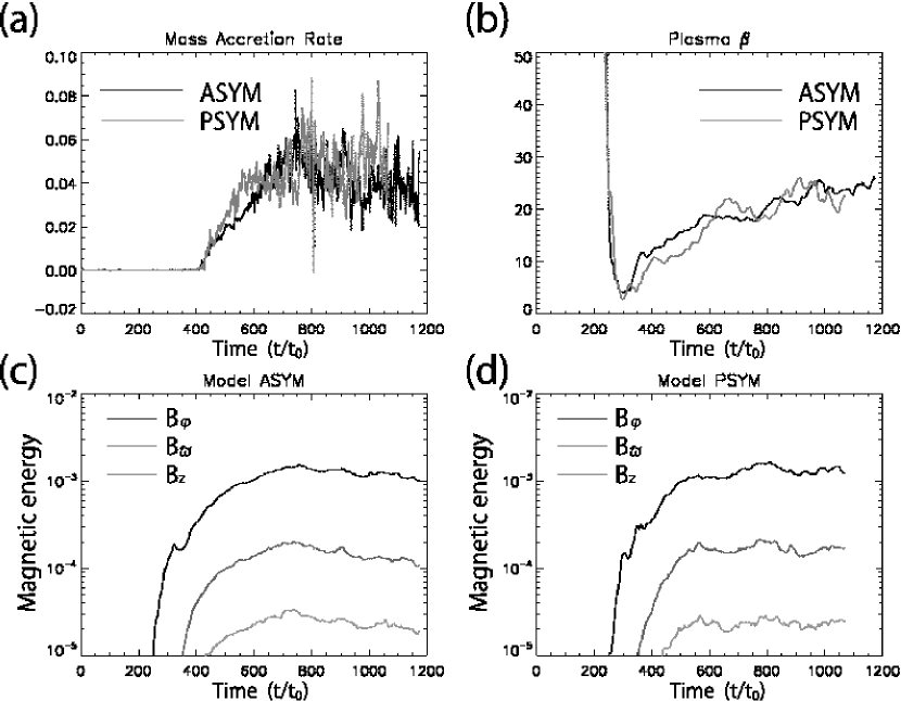
Figure 1: (a) Time evolution of the mass accretion rate at $\varpi/\varpi_{0}=2.5$. Black curve shows model ASYM and gray curve shows model PSYM. (b) Time evolution of the plasma $\beta$ averaged in the region where $2<\varpi/\varpi_{0}<5$, $|z|/\varpi_{0}<1$, and $0\leq\varphi\leq 2\pi$. (c) Time evolution of the spatially averaged magnetic energy of model ASYM. Black, dark gray and gray denotes azimuthal component, radial component and vertical component, respectively. (d) Time evolution of the spatially averaged magnetic energy of model PSYM. Colors are same as in (c). The averaged region of the magnetic energy is same as (b).

Figure 1a shows the time evolution of the mass accretion rate measured at $\varpi/\varpi_{0}=2.5$. After $t/t_{0}\sim 200$, the gas starts to inflow and the mass accretion rate increases linearly. Subsequently ($t/t_{0}>600$) the accretion rate saturates and becomes roughly constant. The evolution of the mass accretion rate in model ASYM (black) is similar to that in model PSYM (gray), where the mass accretion rate for model PSYM is doubled since the model PSYM includes only the region above the equatorial plane.

Figures 1b, 1c and 1d show the time evolution of the plasma $\beta$ and magnetic energy of each component averaged in the region where $2\leq\varpi/\varpi_{0}\leq 5$, $|z|/\varpi_{0}\leq 1$, and $0\leq\varphi\leq 2\pi$, respectively. It is clear that plasma $\beta$ decreases in the linear stage as the magnetic energy increases. In both models, the averaged magnetic energy first increases exponentially. After that, it saturates and becomes roughly constant. Time evolution of magnetic fields is similar between model ASYM and model PSYM. Time evolutions of the growth and saturation in the mass accretion rate are quite similar to those of the averaged magnetic energy. It means that the magnetic turbulence driven by MRI is the main cause of the angular momentum transport which drives mass accretion. In the remaining part of this section, we discuss the results of model ASYM.

In order to check the magnetic fields structure, we analyze the time evolution of mean azimuthal magnetic fields. The mean fields are computed by the same method as Nishikori et al. (2006). Figure 2a shows the time evolution of mean azimuthal magnetic fields. Black curve shows $B_{\varphi}$ averaged in the region where $5<\varpi/\varpi_{0}<6$, $0\leq\varphi\leq 2\pi$, and $0<z/\varpi_{0}<1$, and gray curve shows $B_{\varphi}$ averaged in the region where $5<\varpi/\varpi_{0}<6$, $0\leq\varphi\leq 2\pi$, and $1<z/\varpi_{0}<3$. Black and gray curves correspond to the disk region and halo region, respectively. The azimuthal magnetic fields reverse their direction with timescale $t\sim 300t_{0}\sim 1.5{\rm Gyr}$. This timescale is comparable to that of the buoyant rise of azimuthal magnetic fields. The halo fields also reverse their directions with the same time scale as the disk component.

The radial distribution of the mean azimuthal magnetic fields at $t=1000t_{0}$ are shown in figure 2b. Black and gray curves show the averages in the disk ($0\leq\varphi\leq 2\pi$ and $0<z/\varpi_{0}<1$), and in the halo ($0\leq\varphi\leq 2\pi$ and $1<z/\varpi_{0}<3$), respectively. Since the magnetic fields in the disk becomes turbulent, the direction of azimuthal magnetic fields changes frequently near the equatorial plane. On the other hand, long wavelength magnetic loops are formed in the halo region.

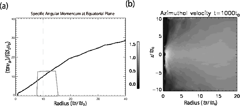
Figure 3: (a) Radial distribution of the specific angular momentum ($l=\varpi v_{\varphi}/(\varpi_{0}v_{0})$) at equatorial plane. Black curve shows the distribution at $t=1000t_{0}$, and gray curve shows the initial condition. Light gray dashed line shows the position of the initial density maximum. (b) Spatial distribution of the azimuthally averaged rotation speed at $t=1000t_{0}$.

Figure 3a shows the radial distribution of the specific angular momentum at equatorial plane. Although the rotation is assumed only inside initial torus (gray curve in figure 3a), torus deforms its shape from a torus to a disk by redistributing angular momentum (black curve in figure 3a). Since the outflow created by the MHD driven dynamo transports angular momentum toward the halo, the halo begins to rotate differentially, as can be seen in iso-contours of the azimuthally averaged rotation speed (figure 3b). Figure 3a and 3b show that the azimuthal velocity $v_{\varphi}$ is almost constant and close to $v_{0}$ in the equatorial plane. The rotation period at $\varpi/\varpi_{0}=a$ is $P_{\rm rot}\sim 2\pi a(\varpi_{0}/v_{0})=2\pi at_{0}$.

3.2 Evolution of the magnetic field structure

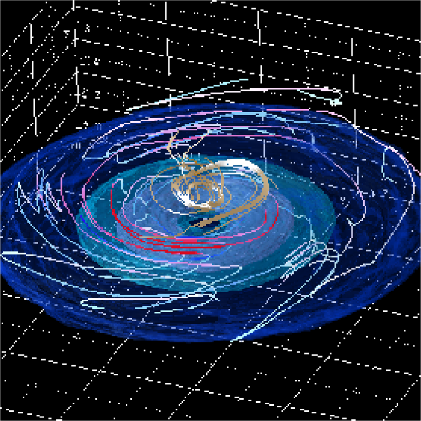
Figure 4: Isosurface of density at $t=1000t_{0}$. The region $|x|/\varpi_{0},|y|/\varpi_{0}<18.5$, and $|z|/\varpi_{0}<7$ is plotted. Curves show the mean magnetic field lines. Color denotes direction of the azimuthal magnetic fields. Blue-white-red corresponds to negative-positive.

We show the 3D structure of mean magnetic fields in figure 4. The colored surfaces represent iso-density surfaces, and the curves show magnetic field lines. Light brown curves show field lines passing through the plane at $z/\varpi_{0}=5$ and $\varpi/\varpi_{0}<1$. The vertical magnetic fields around the rotation axis are produced by the magnetic pressure driven outflow near the galactic center. Color on the curves depicts the direction of azimuthal magnetic fields. Red curves show positive direction of azimuthal magnetic fields (counter clockwise direction) and blue shows negative direction (clockwise). The figure indicates that the azimuthal field reverses the direction with the radius.

Figure 4 indicates that long wavelength magnetic loops are formed around disk-halo interface. Therefore, we discuss the formation mechanism of the magnetic loops. Horizontal magnetic fields embedded in gravitationally stratified atmosphere become unstable against long wavelength undular perturbations. This undular mode of the magnetic buoyancy instability, called Parker instability, creates buoyantly rising magnetic loops (Parker, 1966). Nonlinear growth of Parker instability in gravitationally stratified disks was studied by magneto-hydrodynamic simulations by Matsumoto et al. (1988). They showed that magnetic loops continue to rise when $\beta<5$. In weakly magnetized region where $\beta>5$, Parker instability only drives nonlinear oscillations (Matsumoto et al., 1990).

In differentially rotating disks, MRI couples with Parker instability. The growth time scale of the non-axisymmetric MRI is $t_{\rm MRI}\sim 1/(0.1\Omega)\sim 10H/c_{\rm s}$ where $c_{\rm s}$ is the sound speed. On the other hand, the growth time scale of Parker instability is $t_{\rm PI}\sim 5H/v_{\rm A}\sim 5\sqrt{\beta\gamma/2}(H/c_{\rm s})$ where $v_{\rm A}$ and $\gamma$ are the Alfvén speed and the specific heat ratio, respectively. This time scale becomes comparable to the growth time of MRI when $\beta\sim 5$. Since magnetic turbulence produced by MRI limits the horizontal length of coherent magnetic fields, the growth of Parker instability can be suppressed in weakly magnetized region inside the disk. On the other hand, in regions where $\beta<5$, nonlinear growth of Parker instability creates magnetic loops buoyantly rising to the disk corona (Machida, Hayashi, & Matsumoto, 2000; Machida, et al., 2009).

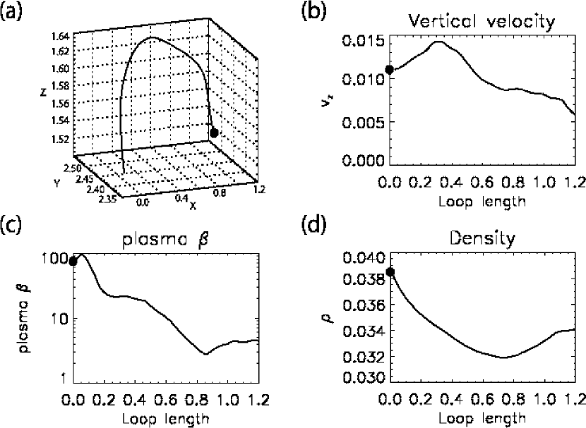
Figure 5: (a) A typical magnetic loop at $t=1000t_{0}$. Black circle denotes the starting point of integration of the magnetic field line. The distribution of the physical quantities along the magnetic field line, (b) vertical velocity, (c) plasma $\beta$, and (d) density, respectively.

Figure 5a shows an example of a magnetic loop at $t=1000t_{0}$. Magnetic loops are identified by the same algorithm as that reported in Machida, et al. (2009). Figure 5b, 5c, and 5d show the distribution of the vertical velocity, plasma $\beta$, and density, respectively along the magnetic field line depicted in figure 5a. A black circle shows the starting point of the integration of a magnetic field line. The positive vertical velocity indicates that the magnetic loop is rising. The value of plasma $\beta$ decreases from the foot-point of the loop where $\beta\sim 100$ to the loop top where $\beta<5$ (figure 5d). The density also decreases from the foot-points to the loop top. These are typical structure of buoyantly rising magnetic loops formed by Parker instability.

From the numerical results presented so far, the initial magnetic field was found to be amplified and transported to the halo region after several rotation periods. In order to investigate the time evolution of the azimuthal magnetic field, we show a butterfly diagram of the azimuthal magnetic fields at $\varpi/\varpi_{0}=2$ (figure 6a). The horizontal axis shows time $t/t_{0}$, and the vertical axis shows the height $z/\varpi_{0}$. Color denotes the direction of the azimuthal magnetic fields. White curve shows the iso-contour where $\beta=5$ above the equatorial plane. We should note that there is no magnetic flux at $\varpi/\varpi_{0}=2$ initially. As the time elapses, the accretion of the interstellar gas driven by MRI transports magnetic fields from $\varpi/\varpi_{0}=10$ to $\varpi/\varpi_{0}=2$. The amplified azimuthal magnetic fields change their directions quasi-periodically. Turbulent magnetic fields are dominant around the equatorial plane.

When the magnetic tension becomes comparable to that of turbulent motion in the disk surface and coherent length of the magnetic field line increases, the magnetic flux buoyantly escapes from the disk due to Parker instability. We find that the instability significantly grows, when the plasma $\beta$ decreases to around 5. The averaged escape velocity of the flux is about 25 km/s, approximately equal to the Alfvén velocity.

The periodic reversals of azimuthal magnetic fields can also be seen in correlation between the fields above and below the equatorial plane (figure 6(b)). White color shows the region where $B_{\varphi}(z)\cdot B_{\varphi}(-z)>0$, and black shows the region where $B_{\varphi}(z)\cdot B_{\varphi}(-z)<0$. We can see fine structures of turbulence near the equatorial plane. In the halo region where $z/\varpi_{0}>1$, the color of outgoing flux changes quasi-periodically. It means that the disk magnetic topology changes between symmetric state and anti-symmetric state.

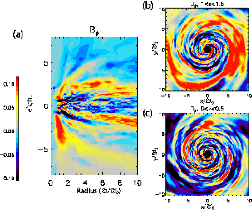
Figure 7: (a) $\varpi-z$ distribution of the azimuthal magnetic fields averaged in the azimuthal direction at $t/t_{0}=1000$. (b) $\varpi-\varphi$ distribution of azimuthal magnetic fields averaged in the vertical direction where $1\leq z/\varpi_{0}\leq 1.5$. (c) $\varpi-\varphi$ distribution of the azimuthal magnetic fields averaged in $0\leq z/\varpi_{0}\leq 0.5$.

Finally, we check the spatial distribution of the azimuthal magnetic fields. The azimuthal magnetic fields in $\varpi-z$ plane averaged in the region $0\leq\varphi\leq 2\pi$ at $t/t_{0}=1000$is shown in figure 7a. We can see that a few $\mu{\rm G}$ fields are distributed as high as at $z/\varpi_{0}=5$. Figure 7b, and 7c show the distribution of the azimuthal magnetic fields in $\varpi-\varphi$ plane, where the azimuthal magnetic fields are averaged in the halo ($1<z/\varpi_{0}<1.5$) and in the disk ($0<z/\varpi_{0}<0.5$), respectively. Since turbulent magnetic fields are dominant inside the disk, short magnetic filaments are formed (figure 7c ). Long and strong azimuthal magnetic sectors are formed in the halo region, because the plasma $\beta$ in the halo region becomes lower than that in the disk due to the density decrease (figure 7b). Therefore, magnetic tension of buoyantly rising magnetic loop exceeds the ram pressure by turbulent motion around the disk surface and in the halo. These magnetic loops buoyantly escape from the disk by Parker instability and create the rising magnetic fluxes in the butterfly diagram shown in figure 6a.

3.3 Dependence on the azimuthal resolution

In order to study the dependence of numerical results on azimuthal resolution, we carried out simulations in which we used 64 (model ASYM64) and 256 (model ASYM256) grid points in $0\leq\varphi\leq 2\pi$. Other parameters are the same as those in model ASYM.

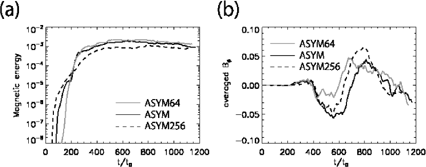
Figure 8: (a) Time evolution of the magnetic energy averaged in the region where $2<\varpi/\varpi_{0}<5$, $|z|/\varpi_{0}<1$, and $0\leq\varphi\leq 2\pi$ . (b) Time evolution of the azimuthal magnetic field averaged in the region where $5<\varpi/\varpi_{0}<6$, $0<z/\varpi_{0}<1$, and $0\leq\varphi\leq 2\pi$. Black, gray, and dashed curves show the results for Model ASYM, ASYM64, and ASYM256, respectively.

Figure 8a shows the time evolution of the magnetic energy averaged in the same region as figure 1c. Black, dashed and gray curves show model ASYM, ASYM256, and ASYM64, respectively. This panel indicates that the saturation level of the magnetic energy near the equatorial plane slightly decreases as the resolution increases because shorter wavelength turbulence inside the disk can be resolved better in the model with higher azimuthal resolution, so that more magnetic energy dissipates in the nonlinear stage. The time evolution of the azimuthal magnetic fields averaged in the region where $5<\varpi/\varpi_{0}<6$, $0<z/\varpi_{0}<1$, and $0\leq\varphi\leq 2\pi$ is shown in figure 8b. Colors are same as figure 8a. The amplitude of the azimuthal magnetic fields and the time scale of the field reversal are almost similar in model ASYM and ASYM256. In order to resolve the most unstable wavelength of MRI, we need more than 20 grid points per disk thickness for azimuthal direction (Hawley, Guan, & Krolik, 2011). Although ASYM does not satisfy this condition, the qualitative behavior of the results for ASYM is identical to that of ASYM256, which satisfies the condition (see figure 8b). For example, the ratio of the radial magnetic energy to the azimuthal magnetic energy ($B_{\varpi}^{2}/B_{\varphi}^{2}$) is $0.12$ in model ASYM and $0.13$ in model ASYM256. Hence, we conclude that numerical results of model PSYM and ASYM in this paper obtained by simulations with 128 grid points in the azimuthal direction do not significantly differ from results with higher azimuthal resolution in the nonlinear stage.

4 Summary and Discussion

We carried out 3D MHD simulations of the galactic gaseous disk. The numerical results indicate that magnetic fields are amplified by MRI. The amplified azimuthal magnetic fluxes buoyantly escape from the disk by Parker instability. Azimuthal component of the mean magnetic field reverses its direction quasi-periodically. The timescale of the reversal is about $300t_{0}$ which corresponds to about 1.5 Gyr.

The numerical results also show that galactic gaseous disk becomes turbulent and that averaged plasma $\beta$ stays at around $\beta\sim 10$. Plasma $\beta$ becomes lower near the disk surface due to the density stratification. Since rotational speed decreases from the disk to the halo (see figure 3b), turbulent magnetic fields are stretched around the disk surface, forming ordered fields. When the magnetic pressure of the ordered fields becomes as large as $\beta\sim 5$, magnetic flux escapes from the disk due to the buoyancy.

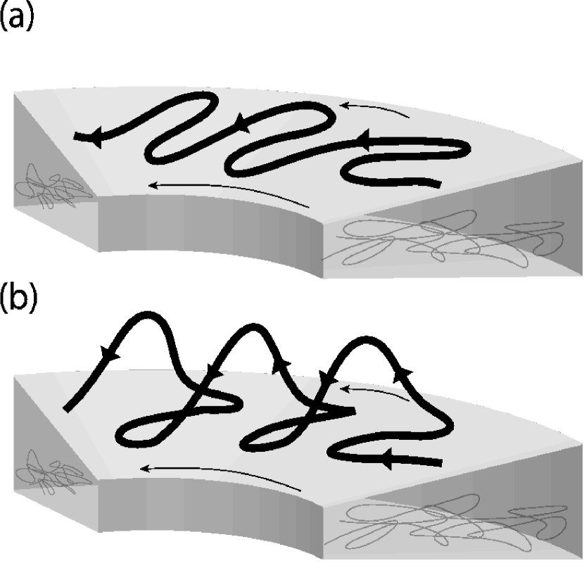
Figure 9: Schematic drawing of the mechanism of MHD Dynamo.

Figure 9 schematically illustrates the mechanism of the galactic dynamo obtained from numerical simulations. Let us consider a differentially rotating disk threaded by weak seed fields, which rotates counter clockwise. As MRI grows in the gaseous disk, positive and negative fields whose strengths are comparable are amplified. When the averaged magnetic pressure becomes about 10% of the gas pressure in the disk, local magnetic pressure near the surface exceeds 20% of the gas pressure and Parker instability creates magnetic loops near the disk surface. Since the magnetic field strength parallel to the seed field grows faster than that of the opposite field, the counter clockwise fields satisfy the condition of Parker instability earlier and buoyantly escape from the disk. Subsequently, clockwise magnetic fields which remain inside the disk are amplified by MRI, and mean azimuthal magnetic fields inside the disk reverses their direction. The reversed fields become a seed field for the next cycle.

Similar quasi-periodic reversal of azimuthal fields have been reported in local 3D MHD simulations of a differentially rotating disk (Shi et al., 2010). Although MRI can grow so long as $\beta\geq 0.1$ (Johansen & Levin, 2008), the saturation level of plasma $\beta$ is about $\beta\sim 1-10$ when the simulations include the effect of the vertical stratification. The growth of MRI saturates when the growth rate of the Parker instability is largest ($\beta\sim 1-10$). It indicates that the saturation levels of the magnetic energy inside the disk is determined by the Parker instability around the surface layer.

Our finding about the periodical reversal of the direction of the halo azimuthal field would impact on the observation of all sky RM map. There are a number of reports about all sky RM distributions (Taylor, Stil, & Sunstrum, 2009; Braun, Heald & Beck, 2010; Han & Zhang, 2007). Study of all sky RM distribution is essential not only to understand the global structure of galactic magnetic fields but also to explore the intergalactic magnetic fields in the intergalactic medium (Akahori & Ryu 2010, 2011, references therein). For instance, Taylor, Stil, & Sunstrum (2009) suggested that the existence of the halo poloidal field is consistent with a dipole field rather than a quadrupole field.

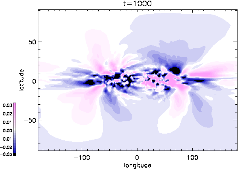
Figure 10: Rotation measure distribution obtained from numerical results.

We calculated the distribution of RM obtained from numerical results (figure 10). The position of the observer is assumed to be at $r=8{\rm kpc}$ at $t=1000t_{0}$. The direction of the rotational velocity and azimuthal magnetic fields is counter-clockwise in our numerical simulation. Since the angular velocity observed in Milky way is clockwise, we calculated the RM distribution by reversing the $z$-direction (i.e. north is $-z$ direction). From the characteristics of MHD, if the initial magnetic field direction were reversed, we can obtain the same result except for the direction of magnetic fields. Thus we reversed the color of the RM from the original one. The scale of RM is arbitrarily in this paper. We found that magnetic loops produced by Parker instability formed multiple reversals of the the sign of RMs along the latitude. These reversals reveal that magnetic fields with opposite polarity emerge from the disk periodically. The snapshot shown in figure 10 indicates that the distribution of RM is point symmetric with respect to the galactic center, and that this feature remains in timescale of $\sim 1.5$ Gyr (figure 2a).

Braun et al. (2010) observed RM distributions in nearby galaxies. They also pointed out that the field topology in the upper halo of galaxies is a mixture of axi-symmetric spiral quadrupole field in thick disks and raidally directed dipole field in halos. They suggested that the origin of the dipole components might be a bipolar outflow. Mixed structure was also suggested by recent studies of all-sky RM map (see, e.g., figure 8 of Pshirkov et al. 2011). The RM distribution in the halo region of our numerical results shows an anti-symmetric distribution corresponding to the dipole field.

Outflows are produced by emerging magnetic fluxs driven by Parker instability. The time interval of the buoyant escape of the magnetic flux by Parker instability is about 10 rotational periods which corresponds to the growth timescale of MRI. Since buoyant escape of magnetic flux takes place about 10 cycles during the simulation for $4{\rm Gyr}$ at $\varpi/\varpi_{0}=2$, the disk becomes turbulent enough, and the influence of the initial field directions become negligible. Even when we start simulations with magnetic fields symmetric to the equatorial plane, the direction of the halo fields in the upper and lower hemisphere becomes opposite at $\varpi/\varpi_{0}=2$ as shown in figure 6a. On the other hand, the effect of the initial field topology still remains in the outer disk region. Since RM is the sum of the line of sight value, the high latitude region (i.e., magnetic loops in nearby disks) still memorizes initial fields. Since the outflow velocity may be faster when we include the effect of the super nova explosions (Wada & Norman, 2001) and the cosmic ray pressure (Kuwabara, Nakamura, & Ko, 2004; Hanasz, Wóltański, & Kowalik, 2009), outer disks may have enough time to create halo fields by the buoyant escape of turbulent disk fields, and eliminate the effect of the initial fields.

Our numerical calculation showed that initially non-rotating halo rotates after several rotation periods, because the angular momentum was supplied from the disk to halo by rising magnetic loops formed by the Parker instability. In fact, HI observation of late type spiral galaxy, NGC 6503 indicated that there were two components of HI disk, thin dense disk and thick low density disk, and that the thick low-density disk rotates slower than the thin disk (Greisen et al., 2009). The rotation speed of the ionized gas in the thick disk is slower than that of HI (Bottema, 1989).

In this paper, we assumed that the interstellar gas is one component gas with temperature $2\times 10^{5}$ K in order to compare the result with that by Nishikori et al. (2006). However, in realistic galaxy, the interstellar gas has multi-temperature, multi-phase components. In future works, we would like to include the energy input by supernovae, multi-temperature structure of the interstellar gas, and cosmic-rays.

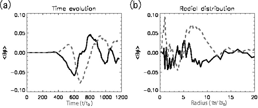
Figure 2: Evolutions of the mean azimuthal magnetic fields averaged in the region where $5<\varpi/\varpi_{0}<6$, $0\leq\varphi<2\pi$, and $0<z/\varpi_{0}<1$ (black), and in the region where $5<\varpi/\varpi_{0}<6$, $0\leq\varphi<2\pi$, and $1<z/\varpi_{0}<3$ (gray). (a) and (b) show time evolution and radial distribution, respectively.

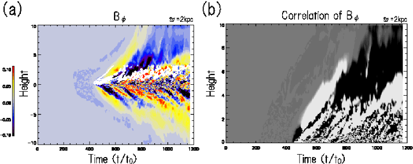
Figure 6: (a) Time evolution of the azimuthal component of magnetic field averaged in the azimuthal direction. White curve shows the location where plasma $\beta=5$ above the equatorial plane $(z>0)$. (b) Correlation of the direction of $B_{\varphi}$ below the equatorial plane and above it. White shows the region of positive correlation where the direction of azimuthal magnetic fields above and below the disk is identical, and black is the region with negative correlation.

References

- Akahori & Ryu (2010) Akahori, K., & Ryu, D. 2010, ApJ, 723, 476
- Akahori & Ryu (2011) Akahori, K., & Ryu, D. 2011, ApJ, 738, 134
- Beck et al. (1996) Beck, R., Brandenburg, A., Moss, D., Shukurov, A., & Sokoloff, D., 1996, ARA&A, 34, 155
- Beck (2012) Beck, R., 2012, Space Science Reviews, 2012, 166, 215
- Bottema (1989) Bottema, R., 1989, A&A, 221, 236
- Braun, Heald & Beck (2010) Braun, R., Heald, G., & Beck, R., 2010, A&A, 514, A42
- Balbus & Hawley (1991) Balbus, S., A., & Hawley, J., F., 1991, ApJ, 376, 214
- Crocker et al. (2010) Crocker, R., M., Jones, D., I., Melia, F., Ott, J. & Protheroe, R. J., 2010, nature, 463, 65
- Greisen et al. (2009) Greisen, E. W., Spekkens, K., & van Moorsekm G. A., 2009, AJ, 137, 4718
- Han et al. (2002) Han, J., L., Manchester, R., N., Lyne, A., G., & Qiao, G. J., 2002, ApJ, 570, L17
- Han & Zhang (2007) Han, J., L., & Zhang, S., 2007, A&A, 464, 609
- Hanasz, Wóltański, & Kowalik (2009) Hanasz, M., Wóltański, D., & Kowalik, K. 2009, ApJ, 706,L155
- Hawley, Guan, & Krolik (2011) Hawley, J. F., Guan, X., & Krolik, J. H., 2011, ApJ, 738, 84
- Horiuchi et al. (1988) Horiuchi, T., Matsumoto, R., Hanawa, T., & Shibata, K., 1988, PASJ, 40, 147
- Kuwabara, Nakamura, & Ko (2004) Kuwabara, T., Nakamura, K., E., & Ko, C., M., 2004, ApJ, 607, 828
- Machida, Hayashi, & Matsumoto (2000) Machida, M., Hayashi, M. R., & Matsumoto, R., 2000, ApJ, 532, L67
- Machida, et al. (2009) Machida, M., Matsimoto, R., Nozawa, S., Takahashi, K., Fukui, Y. Kudo, N., Torii, K., Yamamoto, H., Fujishita, M., & Tomisaka, K., 2009, PASJ, 61, 411
- Matsumoto et al. (1988) Matsumoto, R., Horiuchi, T., Shibata, K., & Hanawa, T., 1988, PASJ, 40, 171
- Matsumoto et al. (1990) Matsumoto, R., Hanawa, T., Shibata, K., & Horiuchi, T., 1990, ApJ, 356, 259
- Miyamoto & Nagai (1975) Miyamoto, M., & Nagai, R., 1975, PASJ, 27, 533
- Morris (1990) Morris, M., 1990, IAUS, 140, 361
- Nishikori et al. (2006) Nishikori, H., Machida, M., & Matsumoto, R., 2006, ApJ, 641, 862
- Nishiyama et al. (2009) Nishiyama, S., Tamura, M., Hatano, H., Nagata, T., Kudo, T., Ishii, M., Schödel, R., & Eckart, A., 2009, ApJ, 702, L56
- Novak et al. (2000) Novak, G., Dotson, J. L., Dowell, C. D., Hildebrand, R., H., Renbarger, T., & Schleuning, D., A., 2000, ApJ, 529, 241
- Okada, Fukue & Matsumoto (1989) Okada, R., Fukue, J., & Matsumoto, R., 1989, PASJ, 41, 133
- Parker (1966) Parker, E., N., 1966, ApJ, 145, 811
- Parker (1971) Parker, E., N., 1971, ApJ, 163, 255
- Pshirkov et al. (2011) Pshirkov, M. S., Tinyakov, P. G., Kronberg, P. P., & Newton-McGee, K., J., 2011, ApJ, 738, 192
- Rand & Kulkarni (1989) Rand, R., J., & Kulkarni, R., 1989, ApJ, 343, 760
- Richetmyer & Morton (1967) Richtmyer, R., O., & Morton, K., W., 1967, Differential Methods for Initial Value Problem (2d ed, New York: Wiley)
- Rubin & Burstein (1967) Rubin, E., & Burstein, S., Z., 1967, J. Comput. Phys., 2, 178
- Fujimoto & Sawa (1987) Fujimoto, M., Sawa, T., 1987, PASJ, 39, 375
- Sawa & Fujimoto (1987) Sawa, T., Fujimoto, M., 1987, in Magnetic Fields and Extragalactic Objects, eds. Asséo, E. and Grésillon, D., p165
- Shi et al. (2010) Shi, J., Krolik, J., H., & Hirose, S., 2010, ApJ, 708, 1716
- Sofue, Fujimoto, & Wielebinski (1986) Sofue, Y., Fujimoto, M., & Wielebinski, R., 1986, ARA&A, 24, 459