A Dual Number Approach for Numerical Calculation of derivatives and its use in the Spherical 4R Mechanism

Abstract

This paper proposes a methodology to calculate both the first and second derivatives of a vector function of one variable in a single computation step. The method is based on the nested application of the dual number approach for first order derivatives. It has been implemented in Fortran language, a module which contains the dual version of elementary functions as well as more complex functions, which are common in the field of rotational kinematics. Since we have three quantities of interest, namely the function itself and its first and second derivative, our basic numerical entity has three elements. Then, for a given vector function $f:\mathbb{R}\to\mathbb{R}^{m}$, its dual version will have the form $\tilde{f}:\mathbb{R}^{3}\to\mathbb{R}^{3m}$. As a study case, the proposed methodology is used to calculate the velocity and acceleration of a point moving on the coupler-point curve generated by a spherical four-bar mechanism.

1 Introduction

The calculation of velocity and acceleration is often needed in the fields of physics and engineering. In some cases, there is no possibility to obtain them analytically. In other cases, the analytical result is quite complicated to deal with; in both situations a numerical treatment is desirable. Regarding the field of mechanisms, the calculation of the first and second derivative allows the designer to include the velocity and acceleration in the synthesis of balanced mechanisms, dwell mechanisms, etc., [1, 2, 3, 4, 5, 6, 7].

Usually, the process of calculating a derivative is not difficult. However, for the case of a spherical mechanism, obtaining first and second derivatives of the position vector for the coupler point is not simple. Even when such derivatives can be explicitly obtained, the resulting expressions could be of great complexity and useless for practical purposes. An alternative solution is to numerically calculate such derivatives. Nevertheless, traditional methods for calculating numerical derivatives (finite-differences) are subject to both truncation and subtractive cancellation errors, not to mention that they are not efficient enough to be used in the optimum synthesis of mechanisms. A different approach that is not subject to the above mentioned errors is automatic differentiation (AD) [8], an algorithmic approach to obtain derivatives for functions which are implemented in computer programs. AD can be implemented in several ways [9], but the use of dual numbers is specially suited for that, since the chain rule can be implemented almost directly.

Analogous to the definition of a complex number $z=a+i\,b$ with $a$ and $b$ being real numbers and $i^{2}=-1$, a dual number is defined as $\hat{r}=a+\epsilon\,b$ where $a$ and $b$ are real numbers but $\epsilon^{2}=0$. Although the first applications of the dual number theory to the development of mechanical engineering date back to early XX century [10], and algebra of dual numbers was developed in the late XIX century [11], applications of dual numbers to numerical calculation of derivatives are relatively recent [12, 13, 14]. Since then, a big amount of work regarding applications of dual numbers has been made. They are used to describe finite displacements of rigid and deformable bodies, for the analytical treatment in kinematic and dynamics of spatial mechanisms, for the study of the kinematics, dynamics and calibration of open-chain robot manipulators, for the study of computer graphics, etc. In references [14, 15, 16] there is some bibliography about such studies.

Due to the great applicability of the dual numbers, it is important to develop algorithms implementing their algebra, which has been done in [15]. It is worthwhile to mention reference [16] where some linear dual algebra algorithms are presented. Regarding applications of dual numbers to compute the numerical derivative of functions, we can cite [12, 13, 14]. In [12], dual numbers are used to calculate first order derivatives and in [13] and [14], they are used to calculate second order derivatives by using the operator overloading method.

The aim of this paper is twofold. First, it develops a methodology based on dual numbers where first and second order derivatives are obtained in a single computation step. Second, it obtains the velocity and acceleration of a point moving on the coupler-point curve generated by a spherical four-bar mechanism.

Once the methodology of developing elementary functions in its dual version including its second derivative has been presented, it is straightforward to develop more sophisticated functions such as rotations and numerical solutions to equations. Moreover, as the use of functions in programming languages as C, C++ and Fortran is quite intuitive and easy to codify, we have created a Fortran module where some functions in their dual version, as well as common functions to the field of rotational kinematics are provided. Such a module along with an example of its usage can be downloaded via internet at http://www.meca.cinvestav.mx/personal/cacruz/archivos-ccv/.

The rest of the paper is organized as follows. Section 2 presents the process of calculating numerical derivatives using dual numbers. Section 3 presents the implementation in Fortran language of the dual versions of scalar elementary functions as well as more complicated expressions, such as vector and matrix functions. In section 4 we show how the velocity and acceleration of a point moving on the coupler-point curve generated by a spherical four-bar mechanism are obtained. Finally, section 5 presents the conclusions.

2 Dual numbers and derivatives

A dual number $\hat{r}$ is a number of the form

$$\hat{r}=a+\epsilon\,b,$$ (2.1)

where $a$ (the real part) and $b$ (the dual part) are real numbers and $\epsilon^{2}=0$. As in the case of complex numbers, there is an isomorphism between dual numbers and the real vector space $\mathbb{R}^{2}$. So, a dual number $\hat{r}$ can be defined as ordered pairs

$$\hat{r}=\{a,b\}.$$ (2.2)

The algebraic rules for dual numbers can be found elsewhere in the literature, see for example [11, 17, 16]. Below we present how the dual numbers are used to calculate derivatives of a function.

2.1 First order derivative

Let us consider the Taylor series expansion (2.3) of a function $f:\mathbb{R}\to\mathbb{R}$ about the point $x$, where $h.o.t.$ stands for higher order terms:

$$f(x+h)=f(x)+f^{\prime}(x)h+\frac{f^{\prime\prime}(x)}{2}h^{2}+\dots+h.o.t.$$ (2.3)

Now, let us consider the dual number $\hat{x}=x+\epsilon$, i.e., a dual number where the coefficient of the nilpotent $\epsilon$ is equal to one. Substituting $\hat{x}$ in (2.3), we obtain $\hat{f}(\hat{x})=f(x+\epsilon)=f(x)+f^{\prime}(x)\epsilon.$

Instead of computing over the reals, we compute over the dual numbers and come up with a dual function $\hat{f}=f(x+\epsilon)$ whose real term is the original function $f(x)$ and the coefficient of $\epsilon$ is its derivative $f^{\prime}(x)$. In the notation of (2.2) we may write

$$\hat{f}(\hat{x})=\left\{f(x),f^{\prime}(x)\right\}.$$ (2.4)

Let us exemplify the procedure for computing the dual function, by using the sinusoidal function. Let $f(x)=\sin(x)$ be the function for which the dual function has to be obtained and let $\hat{g}(\hat{x})=\left\{g_{1}(x),g_{2}(x)\right\}$ be a dual function where $g_{1}(x)=g(x)$ and $g_{2}(x)=g^{\prime}(x)$. Then, from (2.4) we obtain

$$\widehat{\sin}(\hat{g}(\hat{x}))=\left\{\sin\left(g_{1}(x)\right),\cos\left(g_{1}(x)\right)g_{2}(x)\right\}.$$ (2.5)

2.2 Second order derivative

The second order derivative can be obtained by applying (2.4) to $f^{\prime}(x)$, that is, stating the dual version of the function $f^{\prime}(x)$ as

$$\hat{f}^{\prime}(x)=\left\{f^{\prime}(x),f^{\prime\prime}(x)\right\}.$$ (2.6)

The relevant information can be stored in a vector of three components. Such a vector will have the information of the function, its first and its second derivative, so we could speak of an extended dual function (to differentiate it from the common dual function which has only two components). We will use the notation

$$\tilde{f}(x)=\left\{f(x),f^{\prime}(x),f^{\prime\prime}(x)\right\}$$ (2.7)

to represent the extended dual version of the original function $f$. The identity function in its extended dual version $\tilde{x}$, has three components and is given by

$$\tilde{x}=\left\{x,1,0\right\}.$$ (2.8)

Let us exemplify the proposed methodology using the sinusoidal function. Let

$$\tilde{g}(\tilde{x})=\left\{g_{1}(x),g_{2}(x),g_{3}(x)\right\}$$

be an extended dual function, where $g_{1}(x)=g(x)$, $g_{2}(x)=g^{\prime}(x)$, $g_{3}(x)=g^{\prime\prime}(x)$. The sinusoidal function in its extended dual version is given by

$$\widetilde{sin}(\tilde{g})= \{\sin(g_{1}),\;\cos(g_{1})\,g_{2},\;-\sin(g_{1})\,g_{2}^{2}\,+\cos(g_{1})\,g_{3}\}$$ (2.9)

where the arguments of the functions are not written to simplify notation. Notice that no matter how complicated the function $g$, Eq. (2.9) ensures that the chain rule will be successfully applied. Thus by writing all the functions in their extended dual version the derivatives will be obtained without the need of traditional methods of finite-differences.

3 Fortran implementation of the extended dual functions

The extended dual functions are defined as arrays of $3m$ components and since we are interested in functions $f:\mathbb{R}\to\mathbb{R}^{m}$, a function $g:\mathbb{R}^{3}\to\mathbb{R}^{3m}$ is required to write the extended dual version of the function $f$. For example, in the case of the sinusoidal function and considering Fortran programming language, the code results as follows:

module sphmodual
Ψcontains
Ψ
function sindual(x) result(f_result)
Ψimplicit none
Ψdouble precision :: f_result(3)
Ψdouble precision, intent(in) ::  x(3)
Ψf_result=[sin(x(1)),cos(x(1))*x(2),-sin(x(1))*x(2)**2 +Ψcos(x(1))*x(3)]
Ψreturn
end function sindual
Ψ
end module sphmodual

For coding purposes we will use fdual instead of $\tilde{f}$, so in the above code sindual means $\widetilde{\sin}$. A simple program calculating the function $f(x)=\sin(\sin(x))$ for $x=1.1$ in its extended dual version is:

program sind
Ψuse sphmodual
Ψimplicit none
Ψdouble precision :: angd(3), res(3)
Ψangd=[1.1d0,1d0,0d0]
Ψres = sindual(sindual(angd))
Ψprint*,res(1),res(2),res(3)
end program sind
 

After compiling and executing the above program, the result is:

 0.777831   0.285073    -0.720138
 

The first component of the output vector corresponds to $f$, the second one to $f^{\prime}$ and the third one to $f^{\prime\prime}$, all of them evaluated at the argument $x=1.1$. The implementation of all of the other elementary functions is straightforward from this example.

3.1 Extended dual version of more complicated objects

It has been shown how elementary functions can be dualized, but there are more complicated objects such as, for example, the vector product, whose extended dual version is required for applications to rotational kinematics. One approach to handle vector functions is to work by components. Let us exemplify for the cross product. The $i$-th component of the cross product of two vectors $\mathbf{a}$ and $\mathbf{b}$ is given by $(\mathbf{a}\times\mathbf{b})_{i}=\varepsilon_{ijk}a_{j}b_{k}$, where $a_{n}$ and $b_{n}$ are the $n$-th component of vectors $\mathbf{a}$ and $\mathbf{b}$, respectively, and $\varepsilon_{ijk}$ is the Levi-Civitta tensor. Notice that summation over repeated indices is assumed.

As the derivative operator is a linear operator, only the extended dual version of the multiplication has to be obtained, but the addition has not. Below we show the Fortran code for the extended dual version of the cross product.

function crossdual(xd,yd) result(f_result)
Ψimplicit none
Ψdouble precision :: f_result(3,3)
Ψdouble precision, intent(in) :: xd(3,3),yd(3,3)
Ψinteger :: j,k
Ψ
Ψf_result = 0d0
Ψ
Ψdo j=1,3
Ψ do k=1,3
Ψ  f_result(1,:) = f_result(1,:) + levic(1,j,k)*proddual(xd(j,:),yd(k,:))
Ψ  f_result(2,:) = f_result(2,:) + levic(2,j,k)*proddual(xd(j,:),yd(k,:))
Ψ  f_result(3,:) = f_result(3,:) + levic(3,j,k)*proddual(xd(j,:),yd(k,:))
Ψ end do
Ψend do

Ψreturn
end function crossdual

In the levic function, the Levi-Civita tensor is coded. In the proddual function, the extended dual version of the scalar product is coded. The code for both functions is included in the downloadable module. The result is a $3\times 3$ matrix where the first column is the real cross product, the second column is the first order derivative of the cross product, and the third column is the second order derivative of the cross product.

For example, let ${\mathbf{v}}(\theta)=\left\{\cos(\theta),\sin(\theta),\theta^{3}\right\}$ and ${\mathbf{w}}(\theta)=\left\{e^{-\theta^{2}},\theta\cos(\theta),\sin(\theta)\right\}$ be two vectors. A program that calculates its extended dual cross product at $\theta=1.1$ is as follows:

program crossp
use sphmodual
implicit none
double precision :: ang(3),v(3,3),w(3,3),thr(3),crsp(3,3)

thr = [3d0,0d0,0d0]
ang = [1.1d0,1d0,0d0]


v(1,:) = cosdual(ang)
v(2,:) = sindual(ang)
v(3,:) = powdual(ang,thr)

w(1,:) = expdual(-proddual(ang,ang))
w(2,:) = proddual(cosdual(ang),ang)
w(3,:) = sindual(ang)

crsp = crossdual(v,w)
print*,crsp(:,1)
print*,crsp(:,2)
print*,crsp(:,3)
end program crossp

Extended dual version of other mathematical objects like dot product, norms, matrix multiplications, rotation matrices, etc., can be implemented in a similar way.

4 First and second derivative in the spherical 4R mechanism

This section presents the application of the proposed methodology to compute the first and second order derivatives of some useful functions in the synthesis of mechanisms. In particular, the examples concern the spherical four bar mechanism shown in Fig. 1. A detailed procedure in order to obtain the coupler-point curve can be found in [18]. Here we reproduce the essential formulas in order to make the paper self-contained. Notice that the notation has been slightly changed in order to have a clear code for the programming functions.

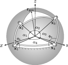
Figure 1: Spherical four-bar mechanism

4.1 Derivative of the output angle

Let us consider the spherical four bar mechanism shown in Fig. 1. Without loss of generality we assume a unit sphere. In its assembly configuration, the input angle is equal to $\Theta_{0}$ and the vectors ${\mathbf{x}}_{k}$ $k=1,2,3,4,$ represent the initial position vectors for the joints $k$, respectively. We will consider the input link as the geodesic connecting the points ${\mathbf{x}}_{1}$ and ${\mathbf{x}}_{2}$, the coupler link as the geodesic connecting the points ${\mathbf{x}}_{2}$ and ${\mathbf{x}}_{3}$, the output link as the geodesic connecting the points ${\mathbf{x}}_{3}$ and ${\mathbf{x}}_{4}$. Finally the fixed link is the geodesic connecting ${\mathbf{x}}_{4}$ and ${\mathbf{x}}_{1}$. Since we are considering a unit sphere, $\alpha_{1}$, $\alpha_{2}$, $\alpha_{3}$, $\alpha_{4}$ will be the lengths of the links, respectively. Once the input link starts to rotate, for example by an angle $\theta$, its new position will be $\Theta_{0}+\theta$. Similarly the position of the output link changes by the amount $\phi(\theta;\vec{\mathbf{x}})$ where the symbol $\vec{\mathbf{x}}$ represents the dependence on ($\mathbf{x}_{1}$, $\mathbf{x}_{2}$, $\mathbf{x}_{3}$, $\mathbf{x}_{4}$). In what follows the dependence of $\phi$ on $\vec{\mathbf{x}}$ will not be written to avoid unnecessary notation, however it will be written in those vectors with such a dependence.

Let ${\mathbf{r}}_{2}(\theta;\mathbf{x}_{1},\mathbf{x}_{2})$ and ${\mathbf{r}}_{3}(\phi(\theta);\vec{\mathbf{x}})$ denote the final positions of input and output link, respectively, given by

$${\mathbf{r}}_{2}(\theta;\mathbf{x}_{1},\mathbf{x}_{2}) ={\mathbf{R}}(\theta,{\mathbf{x}}_{1}){\mathbf{x}}_{2}$$ (4.1)

$${\mathbf{r}}_{3}(\phi(\theta);\vec{\mathbf{x}}) ={\mathbf{R}}(\phi(\theta),{\mathbf{x}}_{4}){\mathbf{x}}_{3},$$ (4.2)

where ${\mathbf{R}}(\vartheta,{\mathbf{x}})$ is a rotation matrix for angle $\vartheta$ about the unit vector ${\mathbf{x}}$.

Since the coupler link must have a constant length, the angle $\phi(\theta)$ can be obtained from

$${\mathbf{r}}_{2}(\theta;\mathbf{x}_{1},\mathbf{x}_{2})\cdot{\mathbf{r}}_{3}(\phi(\theta);\vec{\mathbf{x}})={\mathbf{x}}_{2}\cdot{\mathbf{x}}_{3}=\cos\alpha_{2}=\text{constant}.$$ (4.3)

A closed-form solution of Eq. (4.3) can be found in [19, 20]. In our notation, it is given by

$$\phi=\,\Phi_{0}-2\tan^{-1}\left(\frac{A\pm\sqrt{A^{2}+B^{2}-C^{2}}}{C-B}\right),$$ (4.4)

where

$$A=\, \sin\alpha_{1}\sin\alpha_{3}\sin(\theta+\Theta_{0})$$

$$B=\, \cos\alpha_{1}\sin\alpha_{3}\sin\alpha_{4}-\sin\text{$\alpha_{1}$}\sin\text{$\alpha_{3}$}\cos\text{$\alpha_{4}$}\cos(\theta+\Theta_{0})$$

$$C=\, \sin\text{$\alpha_{1}$}\cos\text{$\alpha_{3}$}\sin\text{$\alpha_{4}$}\cos(\theta+\Theta_{0})+\cos\text{$\alpha_{1}$}\cos\text{$\alpha_{3}$}\cos\text{$\alpha_{4}$}-\cos\text{$\alpha_{2}$}.$$

Although we use Eq. (4.4) to obtain the coupler-point curve generated by the mechanism, in this section, we are interested in showing a numerical approach, where the derivative of $\phi$ with respect to $\theta$ can be found without the analytical knowledge of the $\phi(\theta)$ angle. This can be obtained from $F(\theta,\phi)={\mathbf{r}}_{2}(\theta)\cdot{\mathbf{r}}_{3}(\phi)$, as

$$\frac{d\phi}{d\theta}(\theta)=-\frac{1}{\frac{\partial F}{\partial\phi}(\theta,\phi(\theta))}\,\frac{\partial F}{\partial\theta}(\theta,\phi(\theta)).$$ (4.5)

In order to obtain a numerical value for Eq. (4.5), the $\phi$ angle is obtained by numerically solving Eq. (4.3). Clearly the use of dual numbers is an advantage here, since by implementing the extended dual version of Eq. (4.3) and applying the numerical method of solution also in the context of the extended dual functions, the first and second derivatives of Eq. (4.3) with respect to $\theta$ are automatically obtained, along with the solution for $\phi$. Notice that even when Eq. (4.5) is a formal solution to the problem at hand, yet the derivatives still need to be calculated.

4.2 Velocity and acceleration of the coupler point

We are interested in calculating the velocity and the acceleration of a point moving on the coupler-point curve. Given a mechanism, the only independent (except time dependence) variable is the rotation angle $\theta$ of the input link. Denoting the position vector of the coupler point as $\mathbf{r}_{\text{gen}}$ (see Fig. 2), we have

$$\dot{\mathbf{r}}_{\text{gen}} =\dot{\theta}\,\frac{\partial(\mathbf{r}_{\text{gen}})}{\partial\theta}$$ (4.6)

$$\ddot{\mathbf{r}}_{\text{gen}} =\dot{\theta}^{2}\,\frac{\partial^{2}(\mathbf{r}_{\text{gen}})}{\partial\theta^{2}}+\ddot{\theta}\,\frac{\partial(\mathbf{r}_{\text{gen}})}{\partial\theta},$$ (4.7)

for velocity and acceleration of $\mathbf{r}_{\text{gen}}$. Since one can, in principle, control the angular velocity of the input link, the problem is reduced to calculate $\partial(\mathbf{r}_{\text{gen}})/\partial\theta$ and $\partial^{2}(\mathbf{r}_{\text{gen}})/\partial\theta^{2}$.

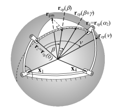
Figure 2: Vectors involved to obtain ${\mathbf{r}}_{\text{gen}}$.

In order to obtain a parametric equation for the coupler-point curve, it is necessary to find the position vector ${\mathbf{r}}_{cp}(\theta,\nu;\vec{{\mathbf{x}}})$ of a point on the coupler link (see Fig. 2). This can be done by rotating the vector ${\mathbf{r}}_{2}(\theta;{\mathbf{x}}_{1},{\mathbf{x}}_{2})$ by an angle $\nu$ about the unit vector $\hat{{\mathbf{n}}}_{23}$ orthogonal to ${\mathbf{r}}_{2}(\theta;{\mathbf{x}}_{1},{\mathbf{x}}_{2})$ and ${\mathbf{r}}_{3}(\phi(\theta);\vec{{\mathbf{x}}})$. Thus

$$\mathbf{r}_{cp}(\theta,\nu;\vec{{\mathbf{x}}})={\mathbf{R}}(\nu,\hat{{\mathbf{n}}}_{23}){\mathbf{r}}_{2}(\theta;{\mathbf{x}}_{1},{\mathbf{x}}_{2})$$ (4.8)

where

$$\hat{\bf{n}}_{23}=\dfrac{{\mathbf{r}}_{2}(\theta;{\mathbf{x}}_{1},{\mathbf{x}}_{2})\times{\mathbf{r}}_{3}(\phi(\theta);\vec{{\mathbf{x}}})}{\lVert{\mathbf{r}}_{2}(\theta;{\mathbf{x}}_{1},{\mathbf{x}}_{2})\times{\mathbf{r}}_{3}(\phi(\theta);\vec{{\mathbf{x}}})\rVert}.$$ (4.9)

Then, the position vector of the coupler point ${\mathbf{r}}_{\text{gen}}$ is obtained by rotating the vector ${\mathbf{r}}_{cp}(\theta,\beta+\gamma;\vec{{\mathbf{x}}})$, being $\gamma$ the angle between ${\mathbf{r}}_{cp}(\theta,\beta;\vec{{\mathbf{x}}})$ and $\mathbf{r}_{\text{gen}}$, by an angle of $\pi/2$ about vector ${\mathbf{r}}_{cp}(\theta,\beta;\vec{{\mathbf{x}}})$:

$${\mathbf{r}}_{\text{gen}}(\theta,\beta,\gamma;\vec{{\mathbf{x}}})={\mathbf{R}}\left(\pi/2,{\mathbf{r}}_{cp}(\theta,\beta;\vec{{\mathbf{x}}})\right){\mathbf{r}}_{cp}(\theta,\beta+\gamma;\vec{{\mathbf{x}}}).$$ (4.10)

So, writing the Eq. (4.10) in its extended dual version, we could automatically get the parametric equation for the coupler-point curve, as well as its first and second derivatives with respect to $\theta$. It is worthwhile to mention that all the necessary functions to obtain ${\mathbf{r}}_{\text{gen}}$ in its extended dual form are coded in the downloadable module.

As a practical example, let us consider the spherical four bar mechanism whose parameters are shown in Table 1. This mechanism was synthesized for the path generation task in [18]. The desired points were firstly presented in [21] and normalized in [22].

Table 1: Parameters of the Spherical 4R mechanism

$\mathbf{x}_{1}$				$\mathbf{x}_{4}$			$\alpha_{1}$	$\alpha_{2}$	$\alpha_{3}$	$\beta$	$\gamma$
1.00000	0.00000	0.00000		0.54462	0.80817	0.22413	0.40144	0.82034	0.92504	0.23067	0.47437

Table 2 shows numerical results for velocity and acceleration, of a point moving on the coupler-point curve as function of the input angle $\theta$.

Table 2: Components of velocity vector $\dot{{\mathbf{r}}}_{\text{gen}}(\theta)$ and acceleration vector $\ddot{{\mathbf{r}}}_{\text{gen}}(\theta)$ for $\dot{\theta}=1$ (units are in the SI system)

$\theta$	$\dot{x}_{\text{gen}}(\theta)$	$\dot{y}_{\text{gen}}(\theta)$	$\dot{z}_{\text{gen}}(\theta)$	$\ddot{x}_{\text{gen}}(\theta)$	$\ddot{y}_{\text{gen}}(\theta)$	$\ddot{z}_{\text{gen}}(\theta)$
$0.00000$	$-0.14255$	$-0.06884$	$0.59467$	$-0.42870$	$-0.25131$	$0.02053$
$0.62832$	$-0.28008$	$-0.18548$	$0.35545$	$0.03897$	$-0.15048$	$-0.56498$
$1.25664$	$-0.17827$	$-0.23972$	$0.05446$	$0.22578$	$-0.00787$	$-0.37389$
$1.88496$	$-0.02698$	$-0.20190$	$-0.13155$	$0.24421$	$0.11368$	$-0.23910$
$2.51327$	$0.10680$	$-0.11271$	$-0.26666$	$0.15791$	$0.16247$	$-0.19681$
$3.14159$	$0.15218$	$-0.00109$	$-0.36590$	$-0.00803$	$0.19437$	$-0.09747$
$3.76991$	$0.12511$	$0.13203$	$-0.36657$	$-0.05418$	$0.22196$	$0.10407$
$4.39823$	$0.09935$	$0.25462$	$-0.23446$	$-0.02558$	$0.14294$	$0.31101$
$5.02655$	$0.08944$	$0.28061$	$0.01394$	$-0.01379$	$-0.08080$	$0.47129$
$5.65487$	$0.05510$	$0.14226$	$0.34717$	$-0.14138$	$-0.34298$	$0.56752$

5 Conclusions

Velocity and acceleration of a coupler-point on a spherical 4R mechanism are obtained by using dual numbers. Although it would be possible to obtain an analytical expression for the position vector of the coupler point, the complexity of the expression does not allow an efficient method to obtain its derivatives, but, if the vector is written in its extended dual version, as it is proposed in this work, its derivatives are obtained directly. As a consequence velocities and accelerations can now be efficiently considered in the optimum synthesis of mechanisms.

The work details the proposal and implementation of a methodology to numerically obtain first and second order derivatives of one variable functions. With our proposal such derivatives (without any approximation) can be obtained in straightforward manner. The methodology is easy to implement and, although we have coded the extended dual functions in the Fortran language, other programming languages could be used.

References

- [1] G. Guj, Z. Dong, M. D. Giacinto, Dimensional synthesis of four bar linkage for function generation with velocity and acceleration constraints, Meccanica: an international journal of theoretical and applied mechanics 16 (4) (1981) 210–219.
- [2] K. Russella, R. S. Sodhib, On the design of slider-crank mechanisms. part I: multi-phase motion generation, Mechanism and Machine Theory 40 (3) (2005) 285–299.
- [3] E. Sandgren, Design of single-and multiple-dwell six-link mechanisms through design optimization., Mechanism and Machine Theory 20 (6) (1985) 483–490.
- [4] Ümit. Sönmez, Introduction to compliant long dwell mechanism designs using buckling beams and arcs, Journal of Mechanical Design 129 (8) (2007) 831 – 844.
- [5] M. Jagannath, S. Bandyopadhyay, A new approach towards the synthesis of six-bar double dwell mechanisms, Computational Kinematics VII (2009) 209–216.
- [6] M. Zobairi, S. Rao, B. Sahay, Kineto-elastodynamic balancing of 4R-four bar mechanisms combining kinematic and dynamic stress considerations, Mechanism and Machine Theory 21 (4) (1986) 307–315.
- [7] Y.-Q. Yu, B. Jiang, Analytical and experimental study on the dynamic balancing of flexible mechanisms, Mechanism and Machine Theory 42 (5) (2007) 626–635.
- [8] R. D. Neidinger, Introduction to automatic differentiation and matlab object-oriented programming, SIAM Review 52 (3) (2010) 545–563.
- [9] A. Griewank, On automatic differentiation, in Mathematical Programming: Recent Developments and Applications, M. Iri and K. Tanabe, eds., Klu wer Academic, Dordrecht, The Netherlands, 1998.
- [10] E. Study, Geometrie der Dynamen, Verlag Teubner, Leipzig, 1903.
- [11] W. Clifford, Preliminary sketch of biquaternions, Proc. London Mathematical Society 1 (s1-4) (1873) 381–395.
- [12] H. Leuck, H.-H. Nagel, Automatic differentiation facilitates of-integration into steering-angle-based road vehicle tracking, IEEE Computer Society Conference on Computer Vision and Pattern Recognition 2 (5) (1999) 2360.
- [13] D. Piponi, Automatic differentiation, c++ templates, and photogrammetry, Journal of graphics, gpu, and game tools 9 (4) (2004) 41–55.
- [14] J. A. Fike, J. J. Alonso (Eds.), The Development of Hyper-Dual Numbers for Exact Second-Derivative Calculations, Proceedings of the 49th AIAA Aerospace Sciences Meeting, Orlando Florida, USA, 2011.
- [15] H. H. Cheng, Programming with dual numbers and its applications in mechanisms design, Engineering with Computers 10 (4) (1994) 212–229.
- [16] E. Pennestrì, P. Valentini, Linear dual algebra algorithms and their application to kinematics, Multibody Dynamics Computational Methods and Applications 12 (2008) 207–229.
- [17] V. Brodsky, M. Shoham, Dual numbers representation of rigid body dinamics, Mechanism and Machine Theory 34 (1999) 975–991.
- [18] F. Peñuñuri, R. Peón-Escalante, C. Villanueva, C. A. Cruz-Villar, Synthesis of spherical 4r mechanism for path generation using differential evolution, Mechanism and Machine Theory 57 (2012) 62–70.
- [19] J. J. Cervantes-Sánchez, H. I. Medellín-Castillo, J. M. Rico-Martínez, E. J. González-Galván, Some improvements on the exact kinematic synthesis of spherical 4r function generators, Mechanism and Machine Theory 44 (2009) 103–121.
- [20] S. Bai, J. Angeles, A unified input-output analysis of four-bar linkages, Mechanism and Machine Theory 43 (2008) 240–251.
- [21] J. Chu, J. Sun, Numerical atlas method for path generation of spherical four-bar mechanism, Mechanism and Machine Theory 45 (2010) 867–879.
- [22] G. Mullineux, Atlas of spherical four-bar mechanisms, Mechanism and Machine Theory 46 (2011) 1811–1823.