Low-energy Electron collisions with O₂: Test of Molecular R-matrix without Diagonalization

Abstract

Electron collisions with O₂ at scattering energies below 1 eV are studied in the fixed-nuclei approximation for a range of internuclear separations using the ab initio molecular R-matrix method. The ${}^{2}\Pi_{\mathrm{g}}$ scattering eigenphases and quantum defects are calculated. The parameters of the resonance and the energy of the bound negative ion are then extracted. Different models of the target that employ molecular orbitals calculated for the neutral target are compared with models based on anionic orbitals. A model using a basis of anionic molecular orbitals yields physically correct results in good agreement with experiment. An alternative method of calculation of the R-matrix is tested, where instead of performing a single complete diagonalization of the Hamiltonian matrix in the inner region, the system of linear equations is solved individually for every scattering energy. This approach is designed to handle problems where diagonalization of an extremely large Hamiltonian is numerically too demanding.

I Introduction

After nitrogen, molecular oxygen is the most abundant molecule in the Earth’s atmosphere. Therefore, its study is crucial to our understanding of planetary atmospheres, while also providing useful insight into the physics of gaseous discharges and laboratory and astrophysical plasmas. Theoretical and experimental research into electron interactions with O₂ has attracted significant scientific attention. Since a complete summary of the relevant references on this topic exceeds the scope of the present study (see the recent review by Itikawa (2009) and references therein), we mention only those directly related to the problem addressed here. An experimental study of the resonant vibrational excitation of O₂ by the low-energy electron impact by Linder and Schmidt (1971) shows oscillatory structures in the cross sections due to the ${}^{2}\Pi_{\mathrm{g}}$ resonance. Celotta et al. (1972) later measured the electron affinity of O₂ using molecular photodetachment spectroscopy. Those two complementary studies Linder and Schmidt (1971); Celotta et al. (1972) provide a deeper understanding of the structure and dynamics of the ${}^{2}\Pi_{\mathrm{g}}$ state of O${}_{2}^{-}$ Parlant and Fiquet-Fayard (1976).

Several previously published theoretical treatments based on the R-matrix method deal with the ${}^{2}\Pi_{\mathrm{g}}$ resonance in the fixed-nuclei approximation Noble and Burke (1986, 1992); Higgins et al. (1994, 1995). All those calculations yield the energy of the ${}^{2}\Pi_{\mathrm{g}}$ resonance at the equilibrium geometry of O₂ more than 0.6 eV above the value obtained from the experimental spectra Linder and Schmidt (1971); Celotta et al. (1972); Teillet-Billy et al. (1987). These studies are unable to reproduce the bound state of O${}_{2}^{-}$ at larger internuclear separations without further adjustments of the R-matrix poles Higgins et al. (1995); Noble et al. (1996). Higgins et al. (1995) used the adjusted results of the ab initio calculations to study resonant vibrational excitation by electron impact and compared the computed cross sections with the experimental work of Field et al. (1988). The resonant vibrational excitation of O₂ at low energies has been revisited by Laporta et al. (2012). Their theoretical treatment of the nuclear motion is based on the “boomerang model” and that utilized the same adjusted positions and widths of the resonances in the fixed-nuclei approximation calculated by Noble et al. (1996).

The energies of the ${}^{2}\Pi_{\mathrm{g}}$ resonance and the bound state of O${}_{2}^{-}$ were later calculated more accurately by Ervin et al. (2003) using the methods of quantum chemistry designed originally for bound states. However, to our knowledge, no reliable ab initio calculation exists that provides reliable scattering phase shifts at low energies ($<2$ eV) for different symmetries.

Significant scientific attention has been paid to electron collisions with O₂ at energies above 2 eV as well. Teillet-Billy et al. (1987) found in their study based on an extended version of multichannel effective range theory that the ${}^{2}\Pi_{\mathrm{g}}$ resonance dominates the electronic excitation of the ${}^{1}\Delta_{\mathrm{g}}$ and ${}^{1}\Sigma_{\mathrm{g}}^{+}$ states. This process was later studied experimentally Allan (1995); Middleton et al. (1992, 1994) and the results confirmed the existence of the resonances predicted by the previous calculations Noble and Burke (1992); Noble et al. (1996); Higgins et al. (1994); Teillet-Billy et al. (1987).

Good correspondence between theoretical and experimental results for the excitation of the ${}^{1}\Delta_{\mathrm{g}}$ and ${}^{1}\Sigma_{\mathrm{g}}^{+}$ electronic states by electron impact has been achieved (see paper Green et al. (2001) and references therein). However, the remaining discrepancies between the theoretical Teillet-Billy et al. (1989); Noble and Burke (1992); Higgins et al. (1994) and experimental cross sections Teillet-Billy et al. (1989); Allan (1995); Green et al. (2001) for excitation of the Herzberg pseudocontinuum (${}^{1}\Sigma_{\mathrm{u}}^{-}$, ${}^{3}\Delta_{\mathrm{u}}$, ${}^{3}\Sigma_{\mathrm{u}}^{+}$) still constitute a challenge Green et al. (2001).

More recently, Tashiro et al. (2006a) presented another R-matrix calculation of the elastic and electronically inelastic electron collisions with O₂ at energies above 5 eV that shows better agreement with the experimental results than previous ab initio studies.

The main goal of the research presented here is to develop an advanced R-matrix calculation of electron collisions with O₂ in the fixed-nuclei approximation at scattering energies below 1 eV. In particular, improvements over previous calculations are sought to provide a more physical energy and width of the ${}^{2}\Pi_{\mathrm{g}}$ resonance and energy of the anionic bound state than was obtained in previous R-matrix studies. The scattering eigenphases and the quantum defects discussed here can be employed in the investigation of the resonant vibrational excitation of O₂ based on the non-local resonance model Domcke (1991) or energy-dependent vibrational frame transformation Gao and Greene (1990). The treatment of bound and continuum states of O${}_{2}^{-}$ introduced here will be later adapted to study other symmetries of the anionic complex that are relevant to O${}_{2}^{-}$ photodetachment and to the vibrational dynamics of that process.

In comparison with previously published ab initio studies, a more physical representation of the anionic complex electronic structure studies is achieved through the use of a more advanced treatment of electron correlation and polarization in the inner region and by employing a basis set of molecular orbitals optimized for the negative ion instead of the neutral target. Note that in other contexts, this idea has also proven to be beneficial Schneider et al. (1979). Current implementations of ab initio electron-molecule scattering theory rely on expansions of the wave functions associated with both the neutral $N$-electron target and the $(N+1)$-electron system which use the same truncated basis of molecular orbitals. Although orbitals optimized for the neutral target are traditionally used in molecular R-matrix calculations, it is far from obvious whether that is universally the most appropriate choice. The present study compares R-matrix calculations performed using optimized neutral target molecular orbitals with those performed using optimized anionic orbitals, in order to ascertain which set is more appropriate.

Another goal of this study is to test the feasibility of an alternative method of calculation of the R-matrix that has the potential to treat larger basis sets and more extensive configuration interaction. The well-established approach preferred in the UK R-matrix codes requires a single full diagonalization of the Hamiltonian matrix in the inner region Tennyson (2010); Carr et al. (2012). The R-matrix is then easily calculated for any scattering energy, since its dependence on the energy is extremely simple in the eigenrepresentation of the Hamiltonian. The development of more efficient R-matrix methods capable of treating molecules having a larger number of active electrons is one of the goals driving this research direction. The requirement of a full Hamiltonian diagonalization in the present implementation has made it quite challenging for the R-matrix method to handle more complex polyatomic molecules and molecules for which electron correlation plays a key role. Evaluation of all the Hamiltonian matrix elements and their storing in the computer memory prior to the full diagonalization is necessary in the present implementation. That approach is computationally much more demanding than the more economical methods of the quantum chemistry of the bound states, where only a small fraction of the spectrum is calculated and the iterative methods of the diagonalization are routinely utilized. Those require only evaluation the matrix elements that are used in the actual iteration. In addition, the complete set of the eigenvectors that have a dense structure is necessary in the present implementation of the ab initio molecular R-matrix method. That further raises issues with the memory limitations.

The method presented in this study employs the solution of a system of linear equations having the same dimension as the Hamiltonian matrix, individually for every scattering energy. A number of other methods have previously been introduced to overcome this difficulty in solving problems requiring very large basis sets. The most promising among them is the partitioned R-matrix Tennyson (2004); Carr et al. (2012). It consists of a single calculation of few lowest eigenvalues and eigenvectors of the Hamiltonian matrix and of a model-like approximation of the rest of the spectrum. While the partitioned R-matrix method retains the advantage of a single diagonalization of a (reduced-dimensionality) Hamiltonian matrix, the alternative method presented here requires solution of the linear system of equations for every scattering energy. However, it is free of any model-like assumptions, and therefore, is a complementary approach to the partitioned R-matrix method. It is hoped, however, that in combination with generalized quantum defect methods or multichannel effective range theory, the quantities to be calculated will be comparatively smooth functions of energy and can accordingly be calculated on a coarse energy mesh. Note that the method of calculation of the R-matrix by solving the system of linear equations has been formulated previously by Collins and Schneider (1981). Their linear-algebraic approach utilizes the static exchange approximation of the electron interactions in the inner region.

The ab initio theoretical description of electron collisions with O₂ at low scattering energies is challenging. Any successful treatment of the complicated polarization effects Hettema et al. (1994); González-Luque et al. (1993) and electron correlation in the inner region requires a large basis set of configurations. Depending on the details of the model, the usual approach based on the full diagonalization of the inner-region Hamiltonian matrix Tennyson (2010); Carr et al. (2012) can become intractable. That makes this system a suitable candidate to test the performance and limitations of the alternative method investigated here. As is discussed below, the linear solution method proves to be feasible and advantageous for calculations where the dimension of the Hamiltonian matrix in the inner region exceeds 40000. Several different models of the target are introduced below and, where possible, the performance of the traditional full diagonalization method is compared with that of the direct linear solution method.

The rest of this paper is organized as follows: Sec. II describes the method adopted to calculate the R-matrix without any diagonalization, by direct solution of a linear inhomogeneous system of equations. Different models of the neutral target are discussed in Sec. III and the construction of the $(N+1)$-electron Hamiltonian matrix is described in Sec. IV. The results are presented in Sec. V and the conclusions are summarized in Sec. VI.

Atomic units are used throughout, unless stated otherwise.

II R-matrix by linear equation solution (LES)

The idea of the R-matrix method is the solution of the Schrödinger equation within a finite reaction volume $\Omega$ of the configuration space. The scattering properties of a many-particle system are known once the normal logarithmic derivative of the wave function and relevant surface amplitudes are specified on the surface $\Sigma$ enclosing the reaction volume. The goal of the theory is to determine this information in the form of an R-matrix. The reaction volume in the molecular ab initio R-matrix method is specified by a sphere of radius $r_{0}$ chosen such that $r_{i}\leq r_{0}$, $r_{i}$ being the distance between the $i$th electron and the center of mass of the molecule. $r_{0}$ is large enough to contain all the complicated interactions of the electrons within the inner region, and sufficiently large that the target wave functions in the open and weakly-closed channels are negligible in the outer region. Interaction of the scattering electron with the target in the outer region is well approximated by the long-range multipole and dispersion potentials that couple different scattering channels Tennyson (2010). The total wave function can be written as Aymar et al. (1996)

$$\Psi_{\beta}(r,\omega)=\sum_{i=1}^{N_{ch}}\frac{1}{r}\Phi_{i}(\omega)F_{i\beta}(r),$$ (1)

where $r$ is the radial coordinate of the scattering electron and $\omega$ denotes all other spin-space coordinates of all the electrons (including the spin and angular coordinates of the scattering one). $\Phi_{i}(\omega)$ includes the electronic state of the target as well as the spherical harmonic of the scattering electron, $F_{i\beta}(r)$ is the scaled radial wave function of the scattering electron in the outer region ($r\geq r_{0}$) in the channel $i$. $N_{ch}$ denotes the total number of scattering channels retained (both open and closed), index $\beta=1,\dots,N_{ch}$ denotes different linearly independent solutions for the total energy $\epsilon$ of interest. If the radial derivative of $F_{i\beta}(r)$ is denoted as $F^{\prime}_{i\beta}(r)$, then the R-matrix on the surface $\Sigma$ is defined Aymar et al. (1996) as

$$\underline{R}=\left(\underline{F}\underline{F}^{\prime-1}\right)_{r_{0}}$$ (2)

and is calculated by solving the Schrödinger equation in the inner region. Then it is used to match the solutions in the outer region and to calculate the $K$-matrix or other quantities that characterize the scattering process Tennyson (2010); Aymar et al. (1996).

The approach to calculation of the R-matrix tested in this work is based on the noniterative variational formulation of the R-matrix method introduced by Ref. Greene (1983) that has been used extensively in a number of problems (see Ref. Aymar et al. (1996) and references therein). Solutions of the time-independent Schrödinger equation at energy $\epsilon$ in the inner region obey

$$\hat{H}\Psi_{\beta}=\epsilon\Psi_{\beta},$$ (3)

where $\hat{H}$ is the electronic Hamiltonian of the $(N+1)$-electron system and $\epsilon$ is the total energy. $\Psi_{\beta}(r,\omega)$ can be expressed using a set of real basis functions $y_{k}(r,\omega)$ as $\Psi_{\beta}(r,\omega)=\sum_{k}y_{k}(r,\omega)C_{k\beta}$. Each of the basis functions $y_{k}$ can be expanded on $\Sigma$ as

$$y_{k}(r_{0},\omega)=\sum_{i=1}^{N_{ch}}\frac{1}{r_{0}}\Phi_{i}(\omega)u_{ik}(r_{0}).$$ (4)

As is well known from Robicheaux (1991) and Greene and Kim (1988), the R-matrix can be expressed as

$$R_{ij}=\sum_{kk^{\prime}}u_{ik}(\Gamma^{-1})_{kk^{\prime}}u_{jk^{\prime}},$$ (5)

where

$$\Gamma_{kk^{\prime}}=2\int_{\Omega}y_{k}(\epsilon-\hat{H}-\hat{L})y_{k^{\prime}}dV.$$ (6)

The integration is performed over the reaction volume $\Omega$. Notice that the matrix $\underline{\Gamma}$ is symmetric due to the presence of the Bloch operator $\hat{L}$ Bloch (1957); Aymar et al. (1996); Tennyson (2010). The basis set used in the UK R-matrix program suite allows for a close-coupling expansion of the total $(N+1)$-electron wave function in the inner region

$$\Psi_{\beta}(r,\omega)=\hat{A}\sum_{i,k}C_{ik\beta}\frac{1}{r}\Phi_{i}(\omega)u_{ik}(r)$$

$$+\sum_{p}D_{p\beta}\chi^{N+1}_{p}(r,\omega),$$ (7)

where $u_{ik}(r)$ are the radial parts of the continuum orbital introduced to represent the scattering electron in the inner region and their values at $r_{0}$ are in general non-zero. The angular parts are included in $\Phi_{i}(\omega)$. The choice of the continuum orbitals depends on the symmetry of the target electronic states. These two are coupled to give the correct overall spin and spatial symmetry of $\Psi_{\beta}(r,\omega)$. Index $i$ denotes the scattering channel in the outer region and characterizes the electronic state of the target as well as the partial wave of the scattering electron. Therefore, each basis function that appears in the first sum in Eq. (7) has non-zero amplitude on the boundary $\Sigma$ and is associated with one scattering channel. Furthermore, the electrons must obey the Pauli principle and they are anti-symmetrized by operator $\hat{A}$. The second summation in Eq. (7) involves antisymmetric $(N+1)$-electron configurations $\chi_{p}^{N+1}$ that have zero amplitude on the boundary $\Sigma$ and where all the electrons occupy the orbitals associated with the target ($L^{2}$ configurations Tennyson (2010)). Notice that in the terminology of the variational R-matrix method Greene (1983); Robicheaux (1991); Aymar et al. (1996) the basis functions in the first sum in Eq. (7) correspond to the open part of the basis, while the second summation corresponds to the closed part.

The eigenstates of the target and the $(N+1)$-electron basis functions are both expressed in terms of the complete active space configuration interaction (CAS CI) Helgaker et al. (2000). It is worth mentioning at this point that the dimension of the ”closed“ part of the basis (second summation in Eq. (7)) is typically much larger than the dimension of the ”open“ part that has non-zero amplitudes on the boundary $\Sigma$.

The modified Hamiltonian matrix for the inner region $\underline{H}_{\Omega}=\underline{H}+\underline{L}$ calculated using the basis expansion (7) is evaluated in the UK R-matrix codes as well as the surface amplitudes $u_{ik}(r_{0})$. The matrix $\underline{\Gamma}$ defined by Eq. 6 can be easily calculated for each scattering energy $\epsilon$ of the interest and Eq. (5) can be used to calculate the R-matrix.

The product $\sum_{k^{\prime}}\left\{\Gamma^{-1}\right\}_{kk^{\prime}}u_{jk^{\prime}}(r_{0})$ is implemented as a solution of the linear system of equations, which is the most computationally demanding step of the calculation.

A celebrated aspect of the approach to the calculation of the R-matrix available in the UK R-matrix suite nowadays is that the matrix $\underline{H}_{\Omega}$ is diagonalized only once and the energy dependence of the R-matrix is calculated analytically Tennyson (2010); Carr et al. (2012); Robicheaux (1991). However, the complete set of eigenvalues and eigenvectors in the given basis set is necessary for accurate evaluation of the R-matrix using the expansion in the eigenstates. Beyond certain size of the basis set the matrix storage hits the memory limit or the time necessary to diagonalize the modified Hamiltonian becomes too long for practical calculations.

The approach based on solution of the linear system for each individual energy of the interest becomes favorable in those cases, since both the time and memory required to solve one system of linear equations is significantly smaller than the time required to completely diagonalize a matrix of the same size. Furthermore, while existing computer routines for complete diagonalization are usually based on the full matrix storage, several modern computer implementations of state of the art linear solvers are based on more economical sparse storage schemes. Since $\underline{H}_{\Omega}$ is often a sparse matrix, the approach introduced above enables calculations that use larger CI models than the diagonalization-based method. A more efficient parallel implementation of the linear solvers than of the algorithms for the complete diagonalization makes the method presented above even more favorable for large-scale calculations performed on high-performance computer clusters. A calculation of the R-matrix for a single value of the energy using Eq. (5) can be executed in the parallel mode in those environments and calculations for multiple energies can be trivially parallelized.

Several other alternatives to the complete diagonalization of $\underline{H}_{\Omega}$ have been proposed and used Beyer et al. (2000); Tennyson (2004); Carr et al. (2012); Tennyson (2010); Tarana and Horáček (2007). They are based on the accurate calculation of a modest number of the lowest eigenvalues and eigenvectors, while the rest of the spectrum is approximated using various models. These approximate approaches preserve the advantage of the single diagonalization and of the analytical energy-dependence of the R-matrix. The most promising method among those is the partitioned R-matrix Tennyson (2004); Carr et al. (2012). The method described above is not based on the diagonalization of $\underline{H}_{\Omega}$ and is free of any model-like assumptions.

III Models of the Neutral Target

All the R-matrix calculations presented here were performed using the polyatomic UKRmol program suite Tennyson (2010); Carr et al. (2012), which uses a basis set of Gaussian-type orbitals (GTOs) in the inner region. The irreducible representations of the $D_{2h}$ point group are used, as this is the largest abelian subgroup of the true $D_{\infty h}$ symmetry point group of O₂. The notation of the $D_{\infty h}$ point group is used throughout the rest of this paper, unless otherwise stated.

The results are presented for a range of internuclear separations from $R_{n}=1.9$ a.u. to $R_{n}=3.5$ a.u., inside of which the potential energy curves for the ground electronic states of both O₂ (${}^{3}\Sigma_{\mathrm{g}}^{-}$) and O${}_{2}^{-}$ (${}^{2}\Pi_{\mathrm{g}}$) reach their minima. The fixed-nuclei scattering phase shifts and smooth quantum defects obtained for that range are essential for future theoretical studies of resonant vibrational excitation by low-energy electrons and these entities also arise in the theoretical description of vibronic coupling in O${}_{2}^{-}$ photodetachment. The molecular orbitals optimized using the state-averaged complete active space self-consistent field (SA-CASSCF) method implemented in the program package MOLPRO Werner and Knowles (1985); Knowles and Werner (1985) are employed in all the R-matrix calculations presented here.

The neutral target is represented by one of two different sets of the molecular orbitals. The first is calculated using an extensive GTO basis set of atomic natural orbitals (ANO) Widmark et al. (1990) and the SA-CASSCF molecular orbitals are optimized for the neutral molecule (three lowest electronic states are averaged with equal weights). This selection of the primary GTO basis set is motivated by Ref. González-Luque et al. (1993), where it was successfully used to calculate the electron affinity of O₂. Furthermore, Jones and Tennyson (2010) found that this GTO basis is necessary to reproduce within CAS CI models the static dipole polarizabilities of various diatomic molecules containing oxygen, although the case of O₂ is not discussed in that study. Previously published R-matrix studies Tashiro et al. (2006a); Higgins et al. (1994) suggest that polarization effects play an important role in the electron collisions with O₂. The ANO basis set is expected to represent these effects more accurately than the more compact Gaussian basis sets employed by the previously published R-matrix calculations. Two different models of neutral O₂ based on the ANO GTO basis and on the neutral molecular orbitals were tested. Two additional models of the target are introduced below, where Dunning’s cc-pVTZ Dunning (1989) GTO basis set is employed. The convergence of the scattering calculations with respect to the size of the CAS and the quality of representation of the correlation and polarization effects can be estimated from comparison of the scattering eigenphases and the energies of the stable negative ion calculated using these different models.

The dominant valence electronic configuration of the ground state of O₂ is

$$(2\sigma_{g})^{2}(2\sigma_{u})^{2}(3\sigma_{g})^{2}(1\pi_{u})^{4}(1\pi_{g})^{2}.$$

It is natural to include the orbitals $3\sigma_{u}$, $2\pi_{g}$ and $2\pi_{u}$ in all the CAS models, since their occupation numbers in the ground state are larger than 0.01. All of the models presented here consist of 8 active valence electrons. The CAS models considered in the previously published R-matrix studies Higgins et al. (1994); Noble and Burke (1992); Tashiro et al. (2006b) include all 12 valence electrons and a smaller set of the active orbitals than the CAS models introduced here. However, our preliminary tests suggest that the correlation effects due to the electrons $2\sigma_{g}$ and $2\sigma_{u}$ can be neglected for the range of the collision energies considered here.

The first CAS model can be expressed as

$$(1\sigma_{g}2\sigma_{g}1\sigma_{u}2\sigma_{u})^{8}(3\sigma_{g}3\sigma_{u}1\pi_{u}2\pi_{u}3\pi_{u}1\pi_{g}2\pi_{g})^{8}.$$ (8)

The R-matrix calculations based on this CAS include the two energetically lowest target states from each irreducible representation that does not contribute to the static dipole polarizability of the ground state. Tashiro et al. (2006b) suggested that the polarization effects were not sufficiently represented in previously published R-matrix studies Noble and Burke (1992); Higgins et al. (1994). As a first step towards the improvement of this deficiency, the 30 lowest states from the irreducible representation ${}^{3}\Pi_{u}$ and the 42 lowest states from the irreducible representation ${}^{3}\Sigma_{u}^{-}$ (both have a non-zero dipole coupling with the ground state) are included in the expansion of the total wave function in the inner region. This set of target states and the CAS expressed by Eq. (8) is denoted as Model 1 in the text below.

In order to evaluate the convergence of the scattering calculations with respect to the number of the active molecular orbitals, another model of the target is introduced. The orbital $3\pi_{u}$ included in Model 1 is replaced by the orbital $4\sigma_{g}$. This CAS can be expressed as

$$(1\sigma_{g}2\sigma_{g}1\sigma_{u}2\sigma_{u})^{8}(3\sigma_{g}4\sigma_{g}3\sigma_{u}1\pi_{u}2\pi_{u}1\pi_{g}2\pi_{g})^{8}.$$ (9)

The R-matrix calculations based on this model include the 40 energetically lowest target states in every symmetry (both singlet and triplet spin states). This model is denoted as Model 2 in the text below.

Table 1: The number of molecular orbitals in every irreducible representation included in different CAS models of the target. The last line shows the number of continuum orbitals (COs) that is the same for all the R-matrix calculations discussed here. The correspondence between the irreducible representations of the point groups $D_{2h}$ and $D_{\infty h}$ is shown as well.

Symmetry ($D_{2h}$)	$a_{g}$	$b_{2u}$, $b_{3u}$	$b_{1g}$	$b_{1u}$	$b_{3g}$, $b_{2g}$	$a_{u}$
Symmetry ($D_{\infty h}$)	$\sigma_{g}$, $\delta_{g}$	$\pi_{u}$	$\delta_{g}$	$\sigma_{u}$, $\delta_{u}$	$\pi_{g}$	$\delta_{u}$
Model 1	3	3	0	3	2	0
Models 2,3	4	2	0	3	2	0
Model 4	4	3	0	3	2	0
COs	37	21	18	21	18	7

The number of molecular orbitals from every irreducible representation included in the treatment of the inner region for every CAS model introduced here is summarized in Table 1.

The scattering eigenphases calculated using the target models introduced above provide insight into the role of the excited electronic states and higher molecular orbitals in electron collisions with O₂. However, they do not yield physically correct energy of the ${}^{2}\Pi_{\mathrm{g}}$ resonance and fail to describe the bound state of O${}_{2}^{-}$. In order to solve this deficiency two additional target models (Models 3 and 4) based on different MOs are introduced. They employ the Dunning cc-pVTZ GTO basis Dunning (1989) and the CASSCF molecular orbitals that are optimized for the ${}^{2}\Pi_{\mathrm{g}}$ ground electronic state of O${}_{2}^{-}$. The choice of the cc-pVTZ basis is motivated by the experience with the R-matrix calculations based on Models 1 and 2 discussed below and by the intention to use the obtained results in the prospective calculations of the nuclear dynamics using the vibrational frame transformation method Gao and Greene (1989, 1990). The R-matrix calculations based on the ANO GTO basis require a rather large R-matrix sphere ($r_{0}=16$ a.u.), which causes numerical difficulties with the vibrational frame transformation method. Models 3 and 4 yield spatially more compact molecular orbitals that can be confined inside the sphere with the radius $r_{0}=10$ a.u. As is discussed below, the R-matrix calculations based on Models 3 and 4 yield at the scattering energies below 1 eV more physical results than the calculations utilizing Models 1 and 2. It should be kept in mind that the molecular orbitals calculated for O${}_{2}^{-}$ do not have any straightforward physical interpretation for the internuclear distances, where the anion is not bound. They are used as the basis functions in the CI expansion of the bound target states and in the expansion of the $(N+1)$-electron scattering wave function, where the correct boundary condition is guaranteed by the continuum orbitals and by the the Bloch operator defined on the boundary of the reaction volume.

Model 3 consists of the same configurations as Model 2 (see Eq. (9)) and 33 target states from every irreducible representation are used in the expansion of the wave function in the inner region. The most complex CAS model constructed in the present study (Model 4) allows the active electrons to occupy both orbitals $4\sigma_{g}$ and $3\pi_{u}$ along with $4\sigma_{u}$. It can be expressed as

$$(1\sigma_{g}2\sigma_{g}1\sigma_{u}2\sigma_{u})^{8}(3\sigma_{g}4\sigma_{g}3\sigma_{u}4\sigma_{u}1\pi_{u}2\pi_{u}3\pi_{u}1\pi_{g}2\pi_{g})^{8}$$ (10)

and it is introduced to study the stability of the R-matrix calculations based on the anionic molecular orbitals with respect to the extension of the CAS. The expansion of the wave function in the inner region includes the 33 lowest target states from every irreducible representation (singlet and triplet spin states) in the R-matrix calculation using this model. The dimension of $\underline{H}_{\Omega}$ for this model is large and its full diagonalization, implemented as a standard method of calculation of the R-matrix in the UK codes Tennyson (2010); Carr et al. (2012) would be numerically very demanding. This suggests that Model 4 is a suitable candidate for demonstrating the alternative approach discussed in Sec. II which employs no diagonalization.

Table 2: Energy of the ${}^{3}\Sigma_{\mathrm{g}}^{-}$ ground electronic state of O₂ (a.u.) and vertical excitation energies (eV) for the lowest few excited states. The excitation energies calculated using Models 1–4 are compared with the experimental values quoted in the reference Teillet-Billy et al. (1987). All the values are for the internuclear separation $R_{e}(O_{2})=2.3$ a.u.

	ANO		cc-pVTZ
State	Model 1	Model 2	Model 3	Model 4	Ref. Teillet-Billy et al. (1987)
${}^{3}\Sigma_{\mathrm{g}}^{-}$	$-149.8557$	$-149.8516$	$-149.8186$	$-149.8430$
${}^{1}\Delta_{\mathrm{g}}$	$1.014$	$1.008$	$1.005$	$1.012$	$0.98$
${}^{1}\Sigma_{\mathrm{g}}^{+}$	$1.871$	$1.828$	$1.815$	$1.822$	$1.65$
${}^{1}\Sigma_{\mathrm{u}}^{-}$	$5.875$	$5.834$	$5.844$	$5.851$	$6.12$
${}^{3}\Delta_{\mathrm{u}}$	$6.141$	$6.094$	$6.099$	$6.124$	$6.27$
${}^{3}\Sigma_{\mathrm{u}}^{+}$	$6.303$	$6.254$	$6.252$	$6.282$	$6.47$
${}^{3}\Sigma_{\mathrm{u}}^{-}$	$9.458$	$9.503$	$9.477$	$9.322$	$9.25$
${}^{1}\Delta_{\mathrm{u}}$	$11.869$	$11.926$	$11.920$	$11.755$	$11.8$

The energy of the ${}^{3}\Sigma_{\mathrm{g}}^{-}$ ground state of O₂ calculated for the equilibrium internuclear separation $R_{e}(\text{O}_{2})=2.3$ a.u. is for Models 1–4 compared in Table 2. Since in Models 1 and 2 the neutral target is represented using a larger ANO GTO basis and the molecular orbitals are optimized for the ground electronic state of the neutral molecule, it is not surprising that these models yield lower energy of the ground state than Models 3 and 4. On the other hand, the highest energy of the O₂ ground state obtained from Model 3 is a consequence of the smaller GTO basis set and of the fact that the wave function of the neutral target is expanded in the truncated basis set of the orbitals optimized for O${}_{2}^{-}$.

The vertical excitation energies for the lowest eight electronic states calculated for Models 1–4 are also compared in Table 2. In general, they are in good agreement with each other. Note that the excitation energy of the lowest excited state ${}^{1}\Delta_{\mathrm{g}}$ is for all the Models 1–4 close to the experimental value quoted in the reference Teillet-Billy et al. (1987). The agreement with the experiment is less convincing for the higher excited states, although the correspondence between Models 1–4 is obvious. Table 2 as well as Table II in the reference Tashiro et al. (2006b) suggests that the change of the primary GTO basis as well as the presence or absence of the orbitals $4\sigma_{g}$ and $3\pi_{u}$ in the CAS do not dramatically affect the vertical excitation energies.

Since one of the goals of the present study is to provide the fixed-nuclei scattering eigenphases and energies of the anionic bound states for a future study of the vibrational dynamics, it is important to represent the target correctly also for different geometries than the equilibrium one. The vibrational energy $\omega_{e}(\text{O}_{2})$ is a suitable quantity that suggests how well the different models introduced above represent the potential energy curve of the ground state near the equilibrium. In fact all the Models 1–4 yield values similar to each other and to the previously published experimental results Ervin et al. (2003). Comparison of Model 1 and Model 3 with the experimental value is shown in Table 3.

Table 3: The equilibrium internuclear distance $R_{e}$, vibrational frequency $\omega_{e}$ of the neutral target and of the ${}^{2}\Pi_{\mathrm{g}}$ anion and the electron affinity $E_{A}$. Calculations based on Model 1 and Model 3 are compared with the experimental results. The non-zero components of the tensor of the static dipole polarizability of the neutral target ($\alpha_{xx}$, $\alpha_{zz}$) at the equilibrium geometry calculated using the same models are compared with previously published theoretical values.

	O2 $(X^{3}\Sigma_{\mathrm{g}}^{-})$			O${}_{2}^{-}$ $(X^{2}\Pi_{\mathrm{g}})$
	Model 1	Model 3	Previously published	Model 1	Model 3	Experimental
			values [Ref.]			values [Ref.]
$R_{e}$ (a.u.)	$2.30$	$2.32$	$2.28\text{ \cite[cite]{\@@bibref{Authors Phrase1YearPhrase2}{Ervin2003}{\@@citephrase{(}}{\@@citephrase{)}}}}$	$2.55$	$2.58$	$2.55\text{ \cite[cite]{\@@bibref{Authors Phrase1YearPhrase2}{Celotta1972}{\@@citephrase{(}}{\@@citephrase{)}}}}$
$\omega_{e}$ (eV)	$0.192$	$0.185$	$0.196\text{ \cite[cite]{\@@bibref{Authors Phrase1YearPhrase2}{Ervin2003}{\@@citephrase{(}}{\@@citephrase{)}}}}$	$0.135$	$0.133$	$0.137\text{ \cite[cite]{\@@bibref{Authors Phrase1YearPhrase2}{Celotta1972}{\@@citephrase{(}}{\@@citephrase{)}}}}$
$\alpha_{xx}$ (a.u.)	$0.08$	$0.22$	$7.12\text{ \cite[cite]{\@@bibref{Authors Phrase1YearPhrase2}{Hettema1994}{\@@citephrase{(}}{\@@citephrase{)}}}}$
$\alpha_{zz}$ (a.u.)	$9.31$	$9.2$	$13.51\text{ \cite[cite]{\@@bibref{Authors Phrase1YearPhrase2}{Hettema1994}{\@@citephrase{(}}{\@@citephrase{)}}}}$
$E_{A}$ (eV)				$-0.408$	$0.375$	$0.448\text{ \cite[cite]{\@@bibref{Authors Phrase1YearPhrase2}{Ervin2003}{\@@citephrase{(}}{\@@citephrase{)}}}}$

As is discussed below, the polarization effects play important role in the scattering at low impact energies. It is their representation that requires rather large number of the target states included in the expansion of the scattering wave function in the inner region. Thus, it is interesting to calculate the static dipole polarizability of the ground state of the neutral molecule to estimate, how well different models introduced above represent these effects. The components of the tensor of the static dipole polarizability $\alpha$ of the ground state $\varphi_{0}$ can be calculated using the sum-over-states formula

$$\alpha_{rs}=\frac{1}{2}\sum_{k>0}\frac{\bra{\varphi_{0}}\hat{d}_{r}\ket{\varphi_{k}}\bra{\varphi_{k}}\hat{d}_{s}\ket{\varphi_{0}}}{\Delta E_{k}}\qquad r,s\in\{x,y,z\},$$ (11)

where $\varphi_{k}$ are the excited states, $\hat{d}_{r,s}$ are the Cartesian components of the operators of the transition dipole moments and $\Delta E_{k}$ is the excitation energy from $\varphi_{0}$ to $\varphi_{k}$. The summation should be performed over the complete set of the eigenstates (only the states of the symmetry ${}^{3}\Pi_{\mathrm{u}}$ or ${}^{3}\Sigma_{\mathrm{u}}^{-}$ have a non-zero contribution) including the continuum states. Here it is performed over all the target states included in the expansion of the scattering wave function in the inner region. The only non-vanishing components of $\alpha$ for the homonuclear diatomic molecule are the diagonal ones $\alpha_{zz}$ and $\alpha_{xx}=\alpha_{yy}$. One can see in Table 3 that Models 1 and 3 yield a similar value of $\alpha_{zz}$ and it is more than 68% of the value that was previously accurately calculated by Hettema et al. (1994). On the other hand, both models yield significantly underestimated value of $\alpha_{xx}$ that is more than one order of magnitude lower than the accurate calculations of Hettema et al. (1994). In fact, all the Models 1–4 introduced above yield very similar values of $\alpha$ and they show rather poor representation of the component that is perpendicular to the internuclear axis. It is worth mentioning that our test calculations (not published here) that utilize the pseudocontinuum orbitals in the CAS in addition to the molecular orbitals Gorfinkiel and Tennyson (2005); Tennyson (2010); Tarana and Tennyson (2008); Jones and Tennyson (2010) yield a higher value of $\alpha_{xx}$. However, the R-matrix calculations with those huge basis sets are computationally too demanding to be practically performed (see also Appendix B).

IV Scattering Calculations

The continuum basis for the inner region is constructed in the polyatomic UKRmol program using additional GTOs with the centers that coincide with the center of the R-matrix sphere. A sufficient number of these GTOs is diffuse enough to have non-zero values on the boundary of the inner region. The exponents are optimized using the program GTOBAS Faure et al. (2002) and the resulting functions are orthogonalized on the set of the molecular orbitals. This procedure yields a set of continuum-type orbitals in the inner region. All the R-matrix calculations presented here include the continuum orbitals with orbital angular momenta $l=0,1,2,3,4,5$. Their number in every irreducible representation is identical for all the Models 1–4 and is listed in Table 1.

Models 1 and 2 are based on the ANO GTO basis that yields quite diffuse molecular orbitals. The corresponding R-matrix calculations require quite a large sphere with radius $r_{0}=16$ a.u. A similarly large R-matrix sphere was also necessary in the R-matrix studies Tarana and Tennyson (2008); Tarana et al. (2009) of electron collisions with other molecules having a sizable polarizability. The GTO basis set cc-pVTZ used in Models 3 and 4 yields target orbitals that are more compact and can be confined within the sphere of the radius $r_{0}=10$ a.u.

The total number of target states (summed over all the irreducible representations and spin states) included in the expansion of the scattering wave function is listed in Table 4 for Models 1–4 along with the dimensions of the corresponding Hamiltonian matrices $\underline{H}_{\Omega}$.

Table 4: The number of the target states $N_{t}$ included in the close-coupling expansion of the total wave function in the inner-region and the dimension of $\underline{H}_{\Omega}$ is compared for Models 1–4. $t_{C}$ is the CPU time in hours required for the calculation of all the matrix elements, $t_{D}$ is the CPU time in hours necessary to diagonalize $H_{\Omega}$ using the LAPACK subroutine DSYEVD and $t_{L}$ is the CPU time in hours necessary to calculate the R-matrix for a single energy using the linear solver PARDISO.

Model	$N_{t}$	Dimension of $\underline{H}_{\Omega}$	$t_{C}$ (h)	$t_{D}$ (h)	$t_{L}$ (h)
1	128	26168	17.7	6.4	0.6
2	640	22456	3.25	3.9	0.92
3	528	22512	4.5	4.17	1.2
4	528	127012	97.7		62.2

Quite a large number of target states are needed to achieve convergence of the scattering $K$-matrix and its eigenphases for all the models discussed here. That, in combination with the large number of the active electrons and orbitals, is the reason for the substantial amount of CPU time required for the evaluation of all the elements of $\underline{H}_{\Omega}$ (see the column $t_{C}$ in Table 4). Note that the CPU time required for the complete diagonalization of $\underline{H}_{\Omega}$ ($t_{D}$ in Table 4) is for Model 2 and 3 comparable with the CPU time necessary for the construction of $\underline{H}_{\Omega}$. The large size of the Hamiltonian matrix for Model 4 dramatically complicates the complete diagonalization of the Hamiltonian matrix and for this case only the method based on solving the linear system of equations was applied. The CPU time required for the solution of the linear system of equations is smaller than the time necessary for the complete diagonalization (see the column $t_{L}$ in Table 4) for all models where both methods can be compared. However, it must be kept in mind that the linear system has to be solved for every scattering energy of interest. This makes the formulation of the outer-region problem in terms of the analytical quantum defects more favorable, since a smooth dependence on the energy permits the R-matrix calculations to be performed for a smaller number of energy grid points followed by interpolation when possible. Also, it should be kept in mind that the repetitive linear equation solution required at different energies is trivially parallelizable. Although the CPU time necessary to calculate the R-matrix for Model 4 using the linear solver is rather high, the efficient parallelization allows for calculating the R-matrix for a single value of the scattering energy on a computer with 8 CPUs in less than 12 hours. The large CPU time required for the construction of $\underline{H}_{\Omega}$ in Model 4 suggests that this is the most time-consuming step of the R-matrix calculation independently of the complete diagonalization.

The large number of $(N+1)$-electron wave functions needed to achieve convergence for all of the Models 1–4 considered here is in fact the usual complication of the ab initio calculations of the electron collisions with molecules with large polarizability Gil et al. (1994). A useful computational method developed to treat this situation efficiently is the R-matrix with pseudostates (RMPS) Gorfinkiel and Tennyson (2005); Tennyson (2010), where the large number of true electronic states of the target is replaced by a smaller set of pseudostates Tarana and Tennyson (2008). We comment, however, that the straightforward application of this approach to the present problem has not simplified the calculations and it does not improve the results. Further details are discussed in Appendix B.

The extensive number of the target states considered in the inner region problem can lead to very time consuming R-matrix propagation in the outer region, if all the scattering channels are included in the outer-region problem (Eq. (1)) as well. This situation is similar to the RMPS calculations, where the R-matrix propagation in the outer region usually requires more CPU time than the complete diagonalization of $\underline{H}_{\Omega}$ Gorfinkiel and Tennyson (2005); Tarana and Tennyson (2008). Fortunately, the treatment of the wave function in the outer region can be simplified. As one can see in Table 2, the threshold energy of the lowest electronically excited channel (${}^{1}\Delta_{\mathrm{g}}$) is at 1 eV above the ground state of O₂. That is the upper limit of the energy range considered in this study. All the scattering channels associated with the excited target states are strongly closed and although they play an important role in the inner region, they can be safely neglected in the outer region.

Since previous R-matrix studies Tarana and Tennyson (2008); Tarana et al. (2009) of the polarization effects suggest that their representation in the inner region plays a more important role than the polarization potential in the outer region, the R-matrix propagation in the outer region is skipped in all the calculations presented here and the R-matrix calculated at $r_{0}$ is used to match directly to the regular and irregular radial wave functions of the free particle in the outer region. Their linear combination determines the $K$-matrix and the scattering eigenphases. The calculations including different numbers of partial waves show that the ${}^{2}\Pi_{\mathrm{g}}$ electronic state of O${}_{2}^{-}$ for the incident electron energies below 1 eV can be sufficiently well-represented in the outer region by the single partial wave $d$, i.e. $l=2$. Therefore, the problem in the outer region problem can be reduced to a single scattering channel. It is worth mentioning at this point that neglecting the long-range interaction of the target with the incident electron in the outer region that is predominated by the polarization potential, leads to a modification of the threshold behavior of the phase shift. While the dependence of the phase shift on the momentum of the incident electron $k$ is is in the present results $\eta(k)\propto k^{5}$ for $k\to 0$, if the potential $\propto r^{-4}$ was taken into account in the outer region, this would not be the leading term in the effective range expansion O’Malley et al. (1961).

The corresponding phase shift $\eta(E)$ for the internuclear separations $R_{n}$, where the electronic state O${}_{2}^{-}$ (${}^{2}\Pi_{\mathrm{g}}$) is not bound, can be parametrized by the Breit-Wigner formula

$$\eta(E)=\tan^{-1}\left(\frac{\Gamma/2}{E_{r}-E}\right)+\eta_{0}(E),$$ (12)

where $\Gamma$ and $E_{r}$ are the width and position of the resonance, respectively and $E=k^{2}/2$ is the kinetic energy of the incident electron. The background phase shift $\eta_{0}(E)$ is a smooth function of the energy and it can be parametrized by a low-order polynomial. This Breit-Wigner fitting formula is only valid for resonance energies well-separated from threshold, i.e. by many widths $\Gamma$.

One of the goals of the present study is to provide the fixed-nuclei data required for the future calculations of the resonant vibrational excitation of O₂ and photodetachment of O${}_{2}^{-}$. To this end the analytical quantum defects $\mu_{0}(E)$ are calculated as a function of the scattering energy for a set of the internuclear separations. The analytical quantum defect $\mu_{0}(E)$ is a scattering quantity similar to the scattering eigenphase $\eta(E)$ in the sense that it specifies the linear combination of the general solutions of the Schrödinger equation in the outer region matching the boundary condition (2). These solutions are rescaled to remove the Wigner threshold factors and the analytical quantum defect is a function of the scattering energy that is smooth across the thresholds and it is well defined for both open and closed channels Greene (1979); Greene et al. (1979). The smooth character of the analytical quantum defects even in the vicinity of the resonance makes this parametrization of the scattering wave functions particularly favorable in the context of the energy-dependent vibrational frame transformation Gao and Greene (1989, 1990).

The reduction of the problem in the outer region to a single scattering channel and to a single partial wave $l=2$ (for incident electron energies below 1 eV) implies that the expansion (1) reduces to a single term. The scaled radial wave function of the scattering electron can be for $r\geq r_{0}$ parametrized as

$$F_{11}(r)=\mathcal{N}\left[f^{0}_{l}(k,r)\cos(\pi\mu^{0})\right.$$

$$\left.-g^{0}_{l}(k,r)\sin(\pi\mu^{0})\right]_{r\geq r_{0}}.$$ (13)

$f^{0}_{l}(k,r)=\sqrt{2/\pi}k^{-l}rj_{l}(kr)$ is the regular scaled radial wave function of the free particle, $g^{0}_{l}(r)=\sqrt{2/\pi}k^{l+1}rn_{l}(kr)$ is the irregular scaled radial wave function, $k$ is the momentum of the incident electron, $j_{l}$ and $n_{l}$ are the regular and irregular spherical Bessel functions, respectively and $\mathcal{N}$ is the normalization factor.

Formulation of the problem in the outer region in terms of the smooth quantum defects $\mu^{0}$ is also favorable for the calculations of the anionic bound states in the fixed-nuclei approximation. For the range of nuclear geometries, where the anionic state is bound, its energy $E_{b}$ can be calculated by solving the equation Greene (1979)

$$\pi\mu^{0}(E_{b})=\pi-\arctan\left[(-2E_{b})^{l+\frac{1}{2}}\right]\qquad E_{b}<0,$$ (14)

where the single partial wave and single target electronic state is assumed. The advantage of this method compared to the widely used matching of the R-matrix to the spherical Hankel functions (see the review Tennyson (2010) and references therein) is that both sides of Eq. (14) are usually smooth functions of energy and the complications due to the poles of the R-matrix can be avoided.

V Results

V.1 The $\mathbf{{}^{2}\Pi_{g}}$ Resonance at Equilibrium Geometry of the Neutral Target

Fig. 1 shows the ${}^{2}\Pi_{\mathrm{g}}$ phase shift for the equilibrium internuclear distance of the neutral target $R_{e}(\text{O}_{2})=2.3$ a.u. calculated using the

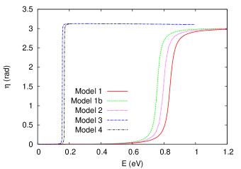
Figure 1: (Color online) The ${}^{2}\Pi_{\mathrm{g}}$ phase shift as a function of the incident electron energy calculated for the internuclear separation $R_{e}(O_{2})=2.3$ a.u. Results for the Models 1–4 are compared.

models introduced in Sec. III. All the curves clearly show a narrow resonance with relatively small background. Model 1 yields the highest resonance position among all ($E_{r}=0.838$ eV). The expansion of the wave function in the inner region includes the 30 lowest target states from the irreducible representation ${}^{3}\Pi_{\mathrm{u}}$ and the 42 lowest target state from the irreducible representation ${}^{3}\Sigma_{\mathrm{u}}^{-}$, since those contribute to the polarizability of the ground state of the target. Only the two lowest target states are included from each of the other irreducible representations that have zero dipole coupling with the ground state of the target.

Further tests showed that the higher target states from these irreducible representations are also important for achieving convergence of the phase shift within the space of configurations (8). The phase shift calculated including the 33 energetically lowest target states from every symmetry in the inner region is plotted in Fig. 1 and denoted as Model 1b. Inclusion of these additional states decreases the resonance position by $0.081$ eV to $E_{r}=0.757$ eV and adding even more excited states does not considerably change this value.

The representation of the polarization effects by the CAS CI model, and the question of how well it is characterized by the static dipole polarizability of the target, has been the subject of several studies Gorfinkiel and Tennyson (2005); Tarana and Tennyson (2008); Tennyson (2010). The difference between the phase shifts denoted as Model 1 and Model 1b in Fig. 1 demonstrates that the static dipole polarizability is not a sufficient measure of the polarization effects in the electron collisions with O₂ at low energies. The decrease of $E_{r}$ with an increasing number of excited target states was also reported by Tashiro et al. (2006b), although that model takes into account only a significantly smaller set of target states; achieving convergence at low energies was not the goal of that study, in any case.

In Model 2, the electrons can occupy the orbital 4$\sigma_{g}$ instead of the orbital 3$\pi_{u}$ included in Model 1. Although the expansion of the wave function in the inner region includes 40 excited states from every irreducible representation, the phase shift shows the resonance at slightly higher collision energy ($E_{r}=0.797$ eV) than Model 1b, as one can see in Fig. 1.

In general, the comparison of the phase shifts calculated using Models 1 and 2 suggests that presence or absence of the molecular orbitals $4\sigma_{g}$ and $3\pi_{u}$ in the CAS does not dramatically affect the parameters of the resonance. The energy of the ${}^{2}\Pi_{\mathrm{g}}$ resonance calculated for $R_{e}(\text{O}_{2})$ using Models 1 and 2 agrees well with the previously published R-matrix calculations by Higgins et al. (1994) ($E_{r}=0.754$ eV). The CAS used in that study is smaller than in Models 1 and 3 and only the eight energetically lowest target states are included in the expansion of the wave function in the inner region. Therefore, none of the target states with $\Pi_{g}$ or $\Pi_{u}$ symmetry are included in that study (see Table 2), although these states have significant contribution to the polarization effects. The absence of the higher molecular orbitals and excited target states is compensated by the virtual orbital that can be singly occupied only in the $(N+1)$-electron wave function Higgins et al. (1994) (the $L^{2}$ configurations in the close-coupling expansion Tennyson (2010) or in Eq. (7)). The use of virtual orbitals raises the issues with the unbalanced treatment of the correlation in the target and in the scattering complex. That can lead to an ambiguity in the energy of the resonance. The models introduced in Sec. III are free of this complication.

The resonance energy $E_{r}$ and width $\Gamma$ calculated for the internuclear separation $R_{e}(\text{O}_{2})$ are summarized in Table 5.

Table 5: Energy $E_{r}$ and width $\Gamma$ of the ${}^{2}\Pi_{\mathrm{g}}$ resonance in O${}_{2}^{-}$ at the equilibrium internuclear distance of the neutral target $R_{e}(\text{O}_{2})$. Results of the molecular R-matrix calculations using Models 1–4 are compared with the results in the previously published references.

	$E_{r}$ (eV)	$\Gamma$ (eV)
Model 1	$0.838$	$0.043$
Model 1b	$0.757$	$0.034$
Model 2	$0.797$	$0.038$
Model 3	$0.154$	$3.6\times 10^{-5}$
Model 4	$0.169$	$1.1\times 10^{-3}$
Higgins et al. (1994)	$0.754$	$0.031$
Noble and Burke (1992)	$0.700$	$0.026$
Derived from experiment Teillet-Billy et al. (1987)	$0.090$	$8.5\times 10^{-5}$

It shows that Models 1 and 2 yield a resonance width $\Gamma$ having the same order of magnitude. These values agree well with the results previously published by Higgins et al. (1994) and by Noble and Burke (1992). Our testing R-matrix calculations performed with even larger CAS than those of Models 1 and 2 (not published here) show that the position and width of the ${}^{2}\Pi_{\mathrm{g}}$ resonance does not considerably change, when both orbitals $3\pi_{u}$ and $4\sigma_{g}$ are included in the CAS.

Although the results obtained using Models 1 and 2 presented in Fig. 1 and Table 5 exhibit encouraging agreement with the previously published R-matrix calculations Higgins et al. (1994); Noble and Burke (1992), they do not agree well with the experimental study by Linder and Schmidt (1971) that found the energy of the ${}^{2}\Pi_{\mathrm{g}}$ resonance to be $E_{r}\approx 0.1$ eV. A similar value was calculated by Ervin et al. (2003) using the stabilization method. This suggests that the relatively good agreement of the phase shifts calculated using Models 1 and 2 points towards the very slow convergence with respect to the number of the molecular orbitals included in the CAS. The authors of the previously published ab initio studies Noble and Burke (1992); Higgins et al. (1994); Tashiro et al. (2006b) attribute the discrepancy between the theoretical and experimental results at energies below 1 eV to the insufficient treatment of the polarization effects, particularly in the outer region. Models 1 and 2 discussed above employ a quite extensive GTO basis set (ANO) that includes a subset of diffuse functions designed to represent the polarization effects. It is reasonable to expect that Models 1 and 2 account for these effects more than in any previously published R-matrix study and the rather large R-matrix sphere ($r_{0}=16\thinspace$ a.u.) should hold most of these effects in the inner region. However, even this improved treatment is not sufficient to provide more physical parameters of the ${}^{2}\Pi_{\mathrm{g}}$ resonance.

The results suggest that the CAS CI representation employing the SA-CASSCF orbitals optimized for the neutral O₂ is not sufficient for the reliable scattering calculations in the energy range considered here. This conclusion is understandable in view of the previously published ab initio studies of the adiabatic electron affinity $E_{A}$ of O₂. It is another essential quantity that characterizes the ${}^{2}\Pi_{\mathrm{g}}$ state of O${}_{2}^{-}$ at the equilibrium internuclear distance of bound O${}_{2}^{-}$ ($R_{e}(\mathrm{O}_{2}^{-})\approx 2.6$ a.u. Ervin et al. (2003)). González-Luque et al. (1993) compared the value of $E_{A}$ calculated using different CI models with the experimental value and found that the methods based on the CAS approach do not yield even a correct sign of $E_{A}$. According to that study, really extensive multi-reference configuration interaction (MRCI) calculations are required to obtain a value of $E_{A}$ comparable with the experimental results. Furthermore, Stampfuß and Wenzel (2003) studied the contributions of the single and double excitations of the reference Hartree-Fock determinants to the binding energy of O${}_{2}^{-}$ (${}^{2}\Pi_{\mathrm{g}}$) and compared it with the contribution of the triple and quadruple excitations. Their results show that both contributions are comparable. Therefore, the set of configurations, where several electrons are excited into the lowest few molecular orbitals (included in the CAS models introduced here), is not sufficient to yield the correct value of $E_{A}$. That requires inclusion of configurations where at least one electron occupies one of the higher molecular orbitals with an orbital number up to 12 in every irreducible representation. These orbitals are not included in the CAS models employed in this study and their further extension would lead to an extremely demanding construction of the Hamiltonian matrix $\underline{H}_{\Omega}$.

Since the equilibrium internuclear separation of O₂ is only 0.3 a.u. smaller than the equilibrium geometry of O${}_{2}^{-}$, the same mechanisms are responsible for the slow convergence of the resonance energy $E_{r}$ at the equilibrium geometry of O₂.

In order to improve the results provided by Models 1 and 2, the CAS Model 3 has been introduced. It employs the SA-CAS MCSCF molecular orbitals of O${}_{2}^{-}$ (${}^{2}\Pi_{\mathrm{g}}$), as is described above. The corresponding phase shift calculated for the internuclear separation $R_{e}(\text{O}_{2})=2.3$ a.u. is also plotted in Fig. 1. It clearly shows a sharp resonance with a relatively smooth background. Fitting to the Breit-Wigner formula (12) yields $E_{r}=0.154$ eV. This value agrees with the experimental results Linder and Schmidt (1971) much better than Models 1 and 2 (see Table 5). The calculation in the inner region includes 33 lowest target states from every irreducible representation and further increase of that number does not considerably change the phase shift. Interpretation of the improvement due to replacement of the orbitals optimized for the neutral target by the anionic molecular orbitals is not straightforward. In general, the orbitals optimized for the anion have more diffuse character than those calculated for the neutral target. Therefore, it is reasonable to expect that they are more suitable to represent the polarization effects than the molecular orbitals of the neutral target. This can partially compensate the absence of the higher orbitals in the CAS models mentioned above. On the other hand, the orbitals calculated for the neutral target are more suitable to represent the ground and excited states of the target than the anionic orbitals used in Model 3. It is possible that the lower energy of the resonance calculated using Model 3 is not only a consequence of the improved treatment of the interaction between the target and the scattering electron, but to some extent also an artifact of less accurate model of the target. In other words, part of the reason of the lower resonance energy in Model 3 is the increase of the target ground state energy with respect to Models 1 and 2 (see Table 2). The CAS CI expansions of the target states and of the $(N+1)$-electron wave function in the same truncated set of the molecular orbitals show different convergence with respect to the number of orbitals and this convergence depends on their character. This general complication of the ab initio R-matrix calculations does not have a universal solution and the particular choice of the molecular orbitals apparently cannot yet be automated, but rather needs to be physically motivated.

The CAS Model 3 yields the vertical excitation energies of the target and the energy of the resonance that are in reasonable agreement with the experimental values (see Table 2 and Table 5). It should be emphasized that these results are not adjusted by an artificial overcorrelation of the $(N+1)$-electron system by introducing virtual orbitals Tennyson (2010); Noble and Burke (1992); Higgins et al. (1994); Tashiro et al. (2006b).

The CAS Model 4 allows the electrons to occupy both $4\sigma_{g}$ and $3\pi_{u}$ molecular orbitals that are included separately in different CAS models introduced previously. In addition, it includes the $4\sigma_{u}$ molecular orbital. This model yields the largest Hamiltonian matrix $\underline{H}_{\Omega}$ among all the Models 1–4 (see Table 4). It is introduced to study the stability of the R-matrix calculations with respect to extending the CAS. The scattering phase shift (plotted in Fig. 1) shows encouraging agreement of the resonance position and width with Model 3, although the energy of the resonance $E_{r}=0.169$ eV is 15 meV higher than the value obtained from Model 3. This slight shift towards higher energies suggests that the molecular orbitals $3\pi_{u}$ and $4\sigma_{u}$ contribute more to the correlation of the target ground state than to the correlation of the $(N+1)$-electron system. The energy of the ground state of the target calculated using Model 4 is 0.66 eV lower than the energy calculated using Model 3 (see Table 2). The good agreement between the $E_{r}$ calculated using Models 3 and 4 suggests that the improvement of the scattering results by employing the anionic molecular orbitals instead of those optimized for the neutral is not purely an artifact due to making the representation of the target worse. The phase shift is rather stable with respect to changes of the CAS that yields different energies of the target states.

Since the construction of the Hamiltonian matrix $\underline{H}_{\Omega}$ in the R-matrix calculations based on the most complex CAS Model 4 is computationally quite demanding (see Table 4), this was performed only for the equilibrium internuclear distance of the neutral target. Since those results show good agreement with the smaller Model 3, that more economical model was used to study the dependence of the ${}^{2}\Pi_{\mathrm{g}}$ bound and continuum states of O${}_{2}^{-}$ on the internuclear distance discussed below.

The effects of the vibrational nuclear dynamics prevent us from directly comparing the cross sections calculated in the fixed-nuclei approximation with experimental results for the energies of the scattering electron below 1 eV. Existence of the bound anionic state (discussed below) leads to well pronounced boomerang oscillations in the elastic scattering cross sections Linder and Schmidt (1971); Higgins et al. (1995); Laporta et al. (2012) that do not appear in the fixed-nuclei calculations. Further theoretical study of these effects using the energy-dependent vibrational frame transformation Gao and Greene (1989, 1990) based on the results presented here will be a subject of the forthcoming research.

V.2 The bound and continuum state of O${}_{2}^{-}$ ($\mathbf{{}^{2}\Pi_{g}}$)

Results of the R-matrix calculations discussed here can be used to study effects of the vibronic coupling in the electron collisions with O₂ or in the photodetachment of O${}_{2}^{-}$. That research requires correct characterization of the bound electronic state of O${}_{2}^{-}$ for a range of the relevant nuclear geometries in addition to the scattering phase shifts or analytical quantum defects. Fig. 2

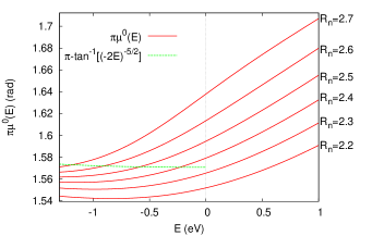
Figure 2: (Color online) Analytical quantum defects $\mu^{0}$ (solid lines) calculated using Model 3 as a function of the incident electron energy $E$ plotted for several internuclear separations $R_{n}$ (a.u.). The right-hand side of Eq. 14 is plotted by the dashed line and the intersections with solid lines determine energies of the O${}_{2}^{-}$ (${}^{2}\Pi_{\mathrm{g}}$) electronic bound state.

shows the analytical quantum defects for several internuclear separations calculated using Model 3 that provides the most physical results at $R_{e}$(O₂). These curves are smooth functions of the incident electron energy, even in the vicinity of the resonance. Relatively slow variation of $\mu^{0}$ with the internuclear separation $R_{n}$ makes this quantity suitable for modeling the vibrational dynamics of the anionic complex based on the energy-dependent vibrational frame transformation Gao and Greene (1990). Fig. 2 also shows the curve corresponding to the right-hand side of Eq. (14). Its intersection with the smooth quantum defect (if it exists) determines the bound-state energy of O${}_{2}^{-}$ (${}^{2}\Pi_{\mathrm{g}}$).

It is well known Ervin et al. (2003); Celotta et al. (1972) that O${}_{2}^{-}$ posses one electronic bound state (${}^{2}\Pi_{\mathrm{g}}$) with the minimum of the potential energy curve below the potential energy minimum of O₂. The potential energy curves of the ground state of neutral O₂ and of the anion calculated using Model 1 and Model 3 are plotted in Fig. 3.

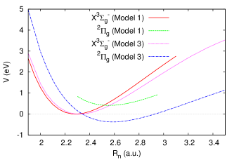
Figure 3: (Color online) Potential energy curves of the target O₂ (${}^{3}\Sigma_{\mathrm{g}}^{-}$) ground electronic state and O${}_{2}^{-}$ (${}^{2}\Pi_{\mathrm{g}}$) state. In the region where the anion is not stable against autodetachment, the anionic curve displayed represents the real part of the corresponding resonance energy. The calculations using Model 1 and Model 3 are compared. The potential energy curves are plotted for each model with respect to energy of the target ground state at its equilibrium nuclear geometry. Model 3 yields a fixed-nucleus electron affinity $E_{A}=0.375$ eV.

The electronic eigenenergies of the anion are calculated using Eq. (14) for the range of the internuclear separations, where the anion is bound and the resonance energy is taken for smaller internuclear distances, where the anionic state has finite lifetime.

Fig. 3 shows that Model 1 does not yield a bound state of the negative ion. Although the anionic potential energy curve crosses the the one of the neutral target at $R\approx 2.51$ a.u., its minimum lies above the minimum of the neutral potential curve. This behavior is common for both Models 1 and 2 and can it is explained above. The R-matrix study by Higgins et al. (1994) also fails to predict the bound state of O${}_{2}^{-}$. The results from the reference Higgins et al. (1994) were later adjusted by shifting the R-matrix poles to reproduce the experimental value of the electron affinity and used to study the resonant vibrational excitation of O₂ by the electron impact Higgins et al. (1995). This sort of shift can lead to an inconsistency between the R-matrix poles and amplitudes that can nonphysically affect the width of the resonance, and has accordingly not been pursued in the present study.

The R-matrix calculations based on Model 3 that employ the molecular orbitals optimized for the negative ion clearly show the bound state of O${}_{2}^{-}$ and yield the electron affinity $E_{A}=0.375$ eV. This is in good agreement with the experimental value 0.448 eV Celotta et al. (1972) supported by later quantum chemical calculation by Ervin et al. (2003) (see also Table 3). The crossing point of the neutral and anionic potential curve obtained using Model 3 is located at internuclear distance 2.34 a.u., very close to the equilibrium geometry of the neutral target. This position is close to that determined in Ref. Ervin et al. (2003). Fig. 4 shows the resonance and bound-state energy of O${}_{2}^{-}$ relatively to the energy of the neutral target ground state. The resonance width as function of $R_{n}$ is plotted in the inset.

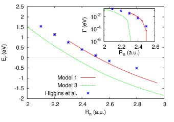
Figure 4: (Color online) The position $E_{r}$ of the ${}^{2}\Pi_{\mathrm{g}}$ state of O${}_{2}^{-}$ calculated as a function of the internuclear distance $R$ plotted with respect to the ${}^{3}\Sigma_{\mathrm{g}}^{-}$ electronic threshold. The results obtained using Model 1 and Model 3 are compared with previously the published calculations by Higgins et al. (1994). The width of the resonance is compared in the inset.

This visualization allows for a direct comparison of Model 1 and Model 3 with Ref. Higgins et al. (1994) for multiple nuclear geometries. It confirms that the good agreement between Model 1 and the reference Higgins et al. (1994) is preserved for other nuclear geometries than the equilibrium of the neutral target, while Model 3 yields lower values of the resonance position and width as well as of the energy of the anionic bound state.

The potential energy curves plotted in Fig. 3 and the analytical quantum defects plotted in Fig. 2 are the central physical results of this study, as well as the basis set configurations that seem to produce the best results. The resonance and bound-state energies of O${}_{2}^{-}$ presented here show that the ab initio R-matrix calculations using Model 3 provide O₂ physically correct eigenphases and smooth quantum defects in the range of the collision energies considered here, in spite of the complicated electronic structure, whereas the previously published ab initio studies provide only inaccurate results.

Another quantities essential in this context are the harmonic vibrational frequencies of the neutral target and of the bound negative ion. As one can see in Table 3, the values obtained using Model 1 and Model 3 are in good agreement with the experimental value Ervin et al. (2003).

VI Conclusion

The ab initio study of the electronic structure of the ${}^{2}\Pi_{\mathrm{g}}$ bound and continuum state of O${}_{2}^{-}$ in the approximation of the fixed nuclei is presented. The scattering eigenphases and the analytical quantum defects are given as functions of the scattering energy for the range of the internuclear separations relevant in the resonant vibrational excitation of O₂ and photodetachment of O${}_{2}^{-}$. The scattering energies below 1 eV, where only one electronic channel is open, are considered. For geometries, where the anionic state is not stable against electron autodetachment, the eigenphases were fitted to the Breit-Wigner formula (12) to determine the resonance position and width. At larger internuclear distances, where the anion is bound, its energy was determined from the smooth quantum defects using Eq. (14). All the calculations were performed using the UK molecular R-matrix program suite Tennyson (2010); Carr et al. (2012).

The results for several different CAS models show that a large basis set of the CI configurations and neutral target eigenstates is necessary in the inner region to achieve converged eigenphases. It is found that if the molecular orbitals of the neutral target are employed in the inner region, the convergence of the CAS model with respect to the number of included orbitals is too slow to provide physically correct characterization of the bound and resonant ${}^{2}\Pi_{\mathrm{g}}$ state of O${}_{2}^{-}$. A different method of selection of the CI configurations other than CAS should be used in that case. However, it is not straightforward to find a more appropriate selection scheme for the CI configurations that treats the target and the $(N+1)$-electron scattering complex in a balanced manner Tennyson (2010); Tarana and Horáček (2007). In addition, any such alternative selection scheme would require substantial changes in the existing UK R-matrix codes. On the other hand, if the molecular orbitals optimized for the negative ion are employed, the CAS approach in the inner region yields the eigenphases and analytical quantum defects that yield the parameters of the resonance and of the bound state in good agreement with the experimental values.

The problem studied here is suitable for a test of the alternative methods of calculation of the R-matrix. The method tested here is based on the solution of the linear system of equations individually for every scattering energy. This method proved more suitable than the single complete diagonalization, when the dimensions of $\underline{H}_{\Omega}$ exceeds 40000, at least for typical computational hardware that is routinely available at present. It represents a nonperturbative alternative to the partitioned R-matrix method that requires a single partial diagonalization of the Hamiltonian matrix $\underline{H}_{\Omega}$ after which the spectrum is completed approximately.

Appendix A Notes on the method used to solve the linear system

The method of calculation of the R-matrix from the Hamiltonian in the inner region $\underline{H}_{\Omega}$ introduced in Sec. II was implemented using the linear solver PARDISO Schenk and Gärtner (2004) that is based on LU factorization. This solver employs a sparse matrix storage scheme and it is designed to handle large and sparse matrices that cannot fully fit into the memory using the full storage. The UK R-matrix program employs the DSYEVD subroutine from the LAPACK library for the complete diagonalization. The DSYEVD subroutine requires storage of the full matrix and does not benefit from the fact that $\underline{H}_{\Omega}$ is usually sparse.

The sparse matrix storage is the main reason, why the method based on solving the system of linear equations is more favorable for large CAS models than the complete diagonalization. When the dimension of $\underline{H}_{\Omega}$ is smaller than $\approx$40000 and when the memory is large enough to store it using the full storage format, the complete diagonalization requires less CPU time than the solution of multiple linear systems for several different scattering energies (see Table 4). Performance of both methods becomes comparable above this dimension and the number of considered scattering energies for which the R-matrix needs to be calculated decides which method requires less CPU time. This dimension is also close to the memory limit of typical contemporary computers. Comparison of both methods beyond this size becomes complicated and considerably larger CAS models can be handled only using methods that do not require full matrix storage.

The CPU time required by PARDISO to solve single system of linear equations also depends on the density of $\underline{H}_{\Omega}$. In general, even very large problem can be solved efficiently using this subroutine, if it is sufficiently sparse.

Appendix B Comment on the application of the RMPS method

The high number of the target states required to achieve a converged expansion of the total $(N+1)$-electron wave function in the inner region naturally suggests that the approach employing the R-matrix with pseudostates (RMPS) method might be rather efficient. Previous studies Gorfinkiel and Tennyson (2005); Tarana and Tennyson (2008); Jones and Tennyson (2010); Tennyson (2010) show that an accurate treatment of the complicated polarization effects in the inner region requires a smaller number of the pseudostates than of the true eigenstates of the target. The RMPS method was applied to the problem studied here and following Gorfinkiel and Tennyson (2005) the singly-excited configurations $(1\sigma_{g}2\sigma_{g}3\sigma_{g}1\sigma_{u}2\sigma_{u}1\pi_{u})^{14}(1\pi_{g})^{1}(\lambda_{i})^{1}$ were included in the CI expansion of the target states, where $\lambda_{i}$ is the pseudocontinuum orbital Gorfinkiel and Tennyson (2005). However, those additional configurations do not have any considerable contribution to the eigenstates of the neutral target in any of Models 1–3, where the RMPS method was tested. As a consequence, the higher pseudostates do not improve the representation of the polarization effects in the scattering calculations.

As an attempt to improve the representation of the pseudostates, the doubly excited configurations, where the pseudocontinuum orbital is singly occupied, were added. These configurations decreased the energies of the target states. Corresponding $(N+1)$-electron terms including the pseudocontinuum orbitals were added to the CI expansion of the $(N+1)$-electron wave function as well. However, this CI model yields an extremely large Hamiltonian $\underline{H}_{\Omega}$ with the dimension exceeding $3\times 10^{5}$. The evaluation of all the matrix elements would require too much CPU time and the R-matrix calculation becomes intractable. Therefore, the RMPS treatment of the electron collisions with O₂ at low incident electron energies should be reconsidered and it will be subject of future research.

References

- Itikawa (2009) Y. Itikawa, J. Phys. Chem. Ref. Data 38, 1 (2009).
- Linder and Schmidt (1971) F. Linder and H. Schmidt, Z. Naturforsch. 26, 1617 (1971).
- Celotta et al. (1972) R. J. Celotta, R. A. Bennett, J. L. Hall, M. W. Siegel, and J. Levine, Phys. Rev. A 6, 631 (1972).
- Parlant and Fiquet-Fayard (1976) G. Parlant and F. Fiquet-Fayard, J. Phys. B: At. Mol. Phys. 9, 1617 (1976).
- Noble and Burke (1986) C. J. Noble and P. G. Burke, J. Phys. B: At. Mol. Phys. 19, L35 (1986).
- Noble and Burke (1992) C. J. Noble and P. G. Burke, Phys. Rev. Lett. 68, 2011 (1992).
- Higgins et al. (1994) K. Higgins, C. J. Noble, and P. G. Burke, J. Phys. B: At. Mol. Opt. Phys. 27, 3203 (1994).
- Higgins et al. (1995) K. Higgins, C. J. Gillan, P. G. Burke, and C. J. Noble, J. Phys. B: At. Mol. Opt. Phys. 28, 3391 (1995).
- Teillet-Billy et al. (1987) D. Teillet-Billy, L. Malegat, and J. P. Gauyacq, J. Phys. B: At. Mol. Phys. 20, 3201 (1987).
- Noble et al. (1996) C. J. Noble, K. Higgins, G. Wöste, P. Duddy, P. G. Burke, P. J. O. Teubner, A. G. Middleton, and M. J. Brunger, Phys. Rev. Lett. 76, 3534 (1996).
- Field et al. (1988) D. Field, G. Mrotzek, D. W. Knight, S. Lunt, and J. P. Ziesel, J. Phys. B: At. Mol. Opt. Phys. 21, 171 (1988).
- Laporta et al. (2012) V. Laporta, R. Celiberto, and J. Tennyson, Unpublished (2012).
- Ervin et al. (2003) K. M. Ervin, I. Anusiewicz, P. Skurski, J. Simons, and W. C. Lineberger, J. Phys. Chem. A 107, 8521 (2003).
- Allan (1995) M. Allan, J. Phys. B: At. Mol. Opt. Phys. 28, 4329 (1995).
- Middleton et al. (1992) A. G. Middleton, P. J. O. Teubner, and M. J. Brunger, Phys. Rev. Lett. 69, 2495 (1992).
- Middleton et al. (1994) A. G. Middleton, M. J. Brunger, P. J. O. Teubner, M. W. B. Anderson, C. J. Noble, G. Wöste, K. Blum, P. G. Burke, and C. Fullerton, J. Phys. B: At. Mol. Opt. Phys. 27, 4057 (1994).
- Green et al. (2001) M. A. Green, P. J. O. Teubner, M. J. Brunger, D. C. Cartwright, and L. Campbell, J. Phys. B: At. Mol. Opt. Phys. 34, L157 (2001).
- Teillet-Billy et al. (1989) D. Teillet-Billy, L. Malegat, J. P. Gauyacq, R. Abouaf, and C. Benoit, J. Phys. B: At. Mol. Opt. Phys. 22, 1095 (1989).
- Tashiro et al. (2006a) M. Tashiro, K. Morokuma, and J. Tennyson, Phys. Rev. A 74, 022706 (2006a).
- Domcke (1991) W. Domcke, Phys. Rep. 208, 97 (1991).
- Gao and Greene (1990) H. Gao and C. H. Greene, Phys. Rev. A 42, 6946 (1990).
- Schneider et al. (1979) B. I. Schneider, M. Le Dourneuf, and V. K. Lan, Phys. Rev. Lett. 43, 1926 (1979).
- Tennyson (2010) J. Tennyson, Phys. Rep. 491, 29 (2010).
- Carr et al. (2012) J. Carr, P. Galiatsatos, J. Gorfinkiel, A. Harvey, M. Lysaght, D. Madden, Z. Mašín, M. Plummer, J. Tennyson, and H. Varambhia, Eur. Phys. J. D 66, 1 (2012).
- Tennyson (2004) J. Tennyson, J. Phys. B: At. Mol. Opt. Phys. 37, 1061 (2004).
- Collins and Schneider (1981) L. A. Collins and B. I. Schneider, Phys. Rev. A 24, 2387 (1981).
- Hettema et al. (1994) H. Hettema, P. E. S. Wormer, P. Jørgensen, H. J. A. Jensen, and T. Helgaker, J. Chem. Phys. 100, 1297 (1994).
- González-Luque et al. (1993) R. González-Luque, M. Merchán, M. P. Fülscher, and B. O. Roos, Chem. Phys. Lett. 204, 323 (1993).
- Aymar et al. (1996) M. Aymar, C. H. Greene, and E. Luc-Koenig, Rev. Mod. Phys. 68, 1015 (1996).
- Greene (1983) C. H. Greene, Phys. Rev. A 28, 2209 (1983).
- Robicheaux (1991) F. Robicheaux, Phys. Rev. A 43, 5946 (1991).
- Greene and Kim (1988) C. H. Greene and L. Kim, Phys. Rev. A 38, 5953 (1988).
- Bloch (1957) C. Bloch, Nucl. Phys. 4, 503 (1957).
- Helgaker et al. (2000) T. Helgaker, P. Jørgensen, and J. Olsen, Molecular electronic-structure theory (Wiley, 2000).
- Beyer et al. (2000) T. Beyer, B. M. Nestmann, and S. D. Peyerimhoff, Chem. Phys. 255, 1 (2000).
- Tarana and Horáček (2007) M. Tarana and J. Horáček, J. Chem. Phys. 127, 154319 (2007).
- Werner and Knowles (1985) H.-J. Werner and P. J. Knowles, J. Chem. Phys. 82, 5053 (1985).
- Knowles and Werner (1985) P. J. Knowles and H.-J. Werner, Chem. Phys. Lett. 115, 259 (1985).
- Widmark et al. (1990) P.-O. Widmark, P.-A. Malmqvist, and B. O. Roos, Theor. Chim. Acta 77, 291 (1990).
- Jones and Tennyson (2010) M. Jones and J. Tennyson, J. Phys. B: At. Mol. Opt. Phys. 43, 045101 (2010).
- Dunning (1989) T. H. J. Dunning, J. Chem. Phys. 90, 1007 (1989).
- Tashiro et al. (2006b) M. Tashiro, K. Morokuma, and J. Tennyson, Phys. Rev. A 73, 052707 (2006b).
- Gao and Greene (1989) H. Gao and C. H. Greene, J. Chem. Phys. 91, 3988 (1989).
- Gorfinkiel and Tennyson (2005) J. D. Gorfinkiel and J. Tennyson, J. Phys. B: At. Mol. Opt. Phys. 38, 1607 (2005).
- Tarana and Tennyson (2008) M. Tarana and J. Tennyson, J. Phys. B: At. Mol. Opt. Phys. 41, 205204 (2008).
- Faure et al. (2002) A. Faure, J. D. Gorfinkiel, L. A. Morgan, and J. Tennyson, Comput. Phys. Commun. 144, 224 (2002).
- Tarana et al. (2009) M. Tarana, B. M. Nestmann, and J. Horáček, Phys. Rev. A 79, 012716 (2009).
- Gil et al. (1994) T. J. Gil, B. H. Lengsfield, C. W. McCurdy, and T. N. Rescigno, Phys. Rev. A 49, 2551 (1994).
- O’Malley et al. (1961) T. F. O’Malley, L. Spruch, and L. Rosenberg, J. Math. Phys. 2, 491 (1961).
- Greene (1979) C. H. Greene, Phys. Rev. A 20, 656 (1979).
- Greene et al. (1979) C. H. Greene, U. Fano, and G. Strinati, Phys. Rev. A 19, 1485 (1979).
- Stampfuß and Wenzel (2003) P. Stampfuß and W. Wenzel, Chem. Phys. Lett. 370, 478 (2003).
- Schenk and Gärtner (2004) O. Schenk and K. Gärtner, Future Gener. Comp. Sy. 20, 475 (2004).