Abstract

In this article, we recalculate the contributions of all vacuum condensates up to dimension-6, in particular the one-loop corrections to the quark condensates $\alpha_{s}\langle\bar{q}q\rangle$ and partial one-loop corrections to the four-quark condensates $\alpha_{s}^{2}\langle\bar{q}q\rangle^{2}$, in the operator product expansion. Then we study the masses and decay constants of the heavy pseudoscalar mesons $D$, $D_{s}$, $B$ and $B_{s}$ using the QCD sum rules with two choices: I we choose the $\overline{MS}$ masses by setting $m=m(\mu)$ and take perturbative corrections up to the order $\mathcal{O}(\alpha_{s})$; II we choose the pole masses $m$, take perturbative corrections up to the order $\mathcal{O}(\alpha_{s}^{2})$ and set the energy-scale to be the heavy quark pole mass $\mu=m_{Q}$. In the case of I, the predictions $f_{D}=(208\pm 11)\,\rm{MeV}$ and $f_{B}=(189\pm 15)\,\rm{MeV}$ are consistent with the experimental data within uncertainties, while the prediction $f_{D_{s}}=(241\pm 12)\,\rm{MeV}$ is below the lower bound of the experimental data $f_{D_{s}}=(260.0\pm 5.4)\,\rm{MeV}$. In the case of II, the predictions $f_{D}=(211\pm 14)\,\rm{MeV}$, $f_{B}=(190\pm 17)\,\rm{MeV}$, $f_{D_{s}}=(258\pm 13)\,\rm{MeV}$ and $f_{D_{s}}/f_{D}=1.22\pm 0.08$ are all in excellent agreements with the experimental data within uncertainties.

PACS number: 13.20.Fc, 13.20.He

Key words: Decay constants, Pseudoscalar mesons, QCD sum rules

1 Introduction

The charged pseudoscalar mesons $\pi^{+}$, $K^{+}$, $D_{s}^{+}$ and $B^{+}$ mesons can decay to a charged lepton pair $\ell^{+}{\nu}_{\ell}$ through a virtual $W^{+}$ boson. To the lowest order, the decay width is

$$\Gamma(P\to\ell\nu) = {{G_{F}^{2}}\over 8\pi}f_{P}^{2}m_{\ell}^{2}m_{P}\left(1-{m_{\ell}^{2}\over m_{P}^{2}}\right)^{2}\left|V_{q_{1}q_{2}}\right|^{2}\,,$$ (1)

where the $m_{P}$ and $f_{P}$ are the mass and decay constant of the pseudoscalar meson, respectively, the $m_{\ell}$ is the $\ell$ mass, the $V_{q_{1}q_{2}}$ is the Cabibbo-Kobayashi-Maskawa matrix element between the constituent quarks $q_{1}\bar{q}_{2}$, and the $G_{F}$ is the Fermi coupling constant. The CLEO collaboration obtains the values $f_{D}=(202\pm 41\pm 17)\,\rm{MeV}$ [1], $(222.6\pm 16.7{}^{+2.8}_{-3.4})\,\rm{MeV}$ [2], $(205.8\pm 8.5\pm 2.5)\,\rm{MeV}$ [3] from the decay $D^{+}\to\mu^{+}\nu_{\mu}$; $f_{D_{s}}=(259.5\pm 6.6\pm 3.1)\,\rm{MeV}$, $f_{D_{s}}/f_{D}=1.26\pm 0.06\pm 0.02$ [4] from the decay $D_{s}^{+}\to\mu^{+}\nu_{\mu}$; $f_{D_{s}}=(252.5\pm 11.1\pm 5.2)\,\rm{MeV}$ [5], $(259.7\pm 7.8\pm 3.4)\,\rm{MeV}$ [6] from the decay $D_{s}^{+}\to\tau^{+}\nu_{\tau}$. The BaBar collaboration obtains the value $f_{D_{s}}=(258.6\pm 6.4\pm 7.5)\,\rm{MeV}$ [7] from the decays $D_{s}^{-}\to\ell^{-}\bar{\nu}_{\ell}$. The Belle collaboration obtains the value $f_{D_{s}}=(275\pm 16\pm 12\,\rm{MeV}$ [8] from the decay $D_{s}^{+}\to\mu^{+}\nu_{\mu}$. Now the average values listed in the Review of Particle Physics are $f_{D}=(206.7\pm 8.9)\,\rm{MeV}$, $f_{D_{s}}=(260.0\pm 5.4)\,\rm{MeV}$ and $f_{D_{s}}/f_{D}=1.26\pm 0.06$ [9].

There have been many theoretical works on the decay constants of the heavy pseudoscalar mesons, such as the QCD sum rules (QCDSR) [10, 11, 12, 13, 14, 15, 16, 17, 18], the lattice QCD (LQCD) [19, 20, 21, 22], the Bethe-Salpeter equation (BSE) [23, 24], the relativistic potential model (RPM) [25, 26, 27], the field-correlator method (FCM) [28], the light-front quark model (LFQM) [29, 30], the chiral extrapolation [31], the extended chiral-quark model [32], etc. There are discrepancies between the theoretical values (from QCDSR and LQCD) and experimental data, which maybe signal some new physics beyond the standard model [15]. In the QCD sum rules for the heavy pseudoscalar mesons, the Wilson coefficients of the vacuum condensates at the operator product expansion side from different references are different from each other in one way or the other, as different authors take different approximations in their calculations [11, 14, 18, 33].

In this article, we recalculate the contributions of all vacuum condensates up to dimension-6, in particular the one-loop corrections to the quark condensates $\alpha_{s}\langle\bar{q}q\rangle$ and partial one-loop corrections to the four-quark condensates $\alpha_{s}^{2}\langle\bar{q}q\rangle^{2}$, in the operator product expansion, take into account all terms neglected in previous works, then study the masses and decay constants of the heavy pseudoscalar mesons $D$, $D_{s}$, $B$ and $B_{s}$ with the QCD sum rules. The QCD sum rules is a powerful theoretical tool in studying the ground state hadrons [34, 35]. The vacuum condensates play an important role in determining the Borel windows, although they maybe play a less important role in the Borel windows. Different Borel windows lead to different ground state masses, therefore different decay constants.

The article is arranged as follows: we derive the QCD sum rules for the masses and decay constants of the heavy pseudoscalar mesons in Sect.2; in Sect.3, we present the numerical results and discussions; and Sect.4 is reserved for our conclusions.

2 QCD sum rules for the heavy pseudoscalar mesons

In the following, we write down the two-point correlation functions $\Pi(p)$ in the QCD sum rules,

$$\Pi(p) = i\int d^{4}xe^{ip\cdot x}\langle 0|T\left\{J_{5}(x)J_{5}^{\dagger}(0)\right\}|0\rangle\,,$$ (2)

$$J_{5}(x) = \bar{Q}(x)i\gamma_{5}q(x)\,,$$ (3)

where the pseudoscalar currents $J_{5}(x)$ interpolate the heavy pseudoscalar mesons, $Q=c,b$ and $q=u,d,s$. We can insert a complete set of intermediate hadronic states with the same quantum numbers as the current operators $J_{5}(x)$ into the correlation functions $\Pi(p)$ to obtain the hadronic representation [34, 35]. After isolating the ground state contributions from the heavy pseudoscalar mesons, we get the following result,

$$\Pi(p) = \frac{f_{P}^{2}m_{P}^{4}}{(m_{Q}+m_{q})^{2}(m_{P}^{2}-p^{2})}+\cdots\,,$$ (4)

where the decay constants $f_{P}$ are defined by

$$\langle 0|J_{5}(0)|P(p)\rangle = \frac{f_{P}m^{2}_{P}}{m_{Q}+m_{q}}\,.$$ (5)

Now, we briefly outline the operator product expansion for the correlation functions $\Pi(p)$ in perturbative QCD, and use the charm-strange (or bottom-strange) mesons to illustrate the procedure. We contract the quark fields in the correlation functions $\Pi(p)$ with Wick theorem firstly,

$$\Pi(p) = i\int d^{4}xe^{ip\cdot x}Tr\left\{\gamma_{5}S_{ij}(x)\gamma_{5}S^{Q}_{ji}(-x)\right\}\,,$$ (6)

where the $S_{ij}(x)$ and $S^{Q}_{ij}(x)$ are the full quark propagators, and can be written as

$$S_{ij}(x) = \frac{i\delta_{ij}\!\not\!{x}}{2\pi^{2}x^{4}}-\frac{\delta_{ij}m_{s}}{4\pi^{2}x^{2}}-\frac{\delta_{ij}}{12}\langle\bar{s}s\rangle+\frac{i\delta_{ij}\!\not\!{x}m_{s}\langle\bar{s}s\rangle}{48}-\frac{\delta_{ij}x^{2}\langle\bar{s}g_{s}\sigma Gs\rangle}{192}+\frac{i\delta_{ij}x^{2}\!\not\!{x}m_{s}\langle\bar{s}g_{s}\sigma Gs\rangle}{1152}$$ (7)

$$-\frac{iG^{a}_{\alpha\beta}t^{a}_{ij}(\!\not\!{x}\sigma^{\alpha\beta}+\sigma^{\alpha\beta}\!\not\!{x})}{32\pi^{2}x^{2}}+\frac{i\delta_{ij}x^{2}\!\not\!{x}g_{s}^{2}\langle\bar{s}\gamma_{\mu}t^{n}s\bar{s}\gamma^{\mu}t^{n}s\rangle}{3456}+\cdots\,,$$

$$S^{Q}_{ij}(x) = \frac{i}{(2\pi)^{4}}\int d^{4}ke^{-ik\cdot x}\left\{\frac{\delta_{ij}}{\!\not\!{k}-m_{Q}}-\frac{g_{s}G^{n}_{\alpha\beta}t^{n}_{ij}}{4}\frac{\sigma^{\alpha\beta}(\!\not\!{k}+m_{Q})+(\!\not\!{k}+m_{Q})\sigma^{\alpha\beta}}{(k^{2}-m_{Q}^{2})^{2}}\right.$$

$$\left.+\frac{g_{s}D_{\alpha}G^{n}_{\beta\lambda}t^{n}_{ij}(f^{\lambda\beta\alpha}+f^{\lambda\alpha\beta})}{3(k^{2}-m_{Q}^{2})^{4}}-\frac{g_{s}^{2}(t^{a}t^{b})_{ij}G^{a}_{\alpha\beta}G^{b}_{\mu\nu}(f^{\alpha\beta\mu\nu}+f^{\alpha\mu\beta\nu}+f^{\alpha\mu\nu\beta})}{4(k^{2}-m_{Q}^{2})^{5}}+\cdots\right\}\,,$$

$$f^{\lambda\alpha\beta} = (\!\not\!{k}+m_{Q})\gamma^{\lambda}(\!\not\!{k}+m_{Q})\gamma^{\alpha}(\!\not\!{k}+m_{Q})\gamma^{\beta}(\!\not\!{k}+m_{Q})\,,$$

$$f^{\alpha\beta\mu\nu} = (\!\not\!{k}+m_{Q})\gamma^{\alpha}(\!\not\!{k}+m_{Q})\gamma^{\beta}(\!\not\!{k}+m_{Q})\gamma^{\mu}(\!\not\!{k}+m_{Q})\gamma^{\nu}(\!\not\!{k}+m_{Q})\,,$$ (8)

and $t^{n}=\frac{\lambda^{n}}{2}$, the $\lambda^{n}$ is the Gell-Mann matrix, the $i$, $j$ are color indexes, $D_{\alpha}=\partial_{\alpha}-ig_{s}G^{n}_{\alpha}t^{n}$ [35]; then compute the integrals both in the coordinate and momentum spaces; finally obtain the correlation functions $\Pi(p)$ at the level of quark-gluon degrees of freedom. In Figs.1-4, we express the contributions of the mixed condensates, four-quark condensates, gluon condensates and three-gluon condensates in terms of Feynman diagrams, which are drawn up directly from Eqs.(6-8). In the Feynman diagrams, we use the solid and dashed lines to represent the light and heavy quark propagators, respectively.

The analytical expressions of the perturbative $\mathcal{O}(\alpha_{s})$ corrections [10] and semi-analytical expressions of the perturbative $\mathcal{O}(\alpha_{s}^{2})$ corrections [12] to the perturbative term are available now. We take into account those analytical and semi-analytical expressions directly [10, 12]; and recalculate the one-loop corrections to the quark condensates. We insert the following term

$$\frac{1}{2!}\,\,ig_{s}\int d^{4}y\bar{\psi}(y)\gamma^{\mu}\psi(y)t^{a}G^{a}_{\mu}(y)\,\,ig_{s}\int d^{4}z\bar{\psi}(z)\gamma^{\nu}\psi(z)t^{b}G^{b}_{\nu}(z)\,,$$ (9)

into the correlation functions $\Pi(p)$ firstly, where the $\psi$ denotes the quark fields, then contract the quark fields with Wick theorem, and extract the quark condensate $\langle\bar{s}{s}\rangle$ according to Eq.(7) to obtain the perturbative corrections $\alpha_{s}\langle\bar{s}{s}\rangle$. There are six Feynman diagrams make contributions, see Fig.5. In summary, we calculate the Feynman diagrams shown explicitly in Figs.1-5 to obtain the contributions of the vacuum condensates in the operator product expansion.

In the following, we will present some necessary technical details in calculations. In this article, we take the light quark mass $m_{q}$ (or $m_{s}$) as a small quantity and expand it perturbatively. In Fig.5, there exist divergences, the quark condensate in the full propagators should be replaced as

$$\frac{\langle\bar{s}s\rangle}{12}\to\frac{\langle\bar{s}s\rangle}{3D}=\frac{\langle\bar{s}s\rangle}{12}\left(1+\frac{1}{2}\epsilon\right)\,.$$ (10)

In this article, we carry out the integrals in the dimension $D=4-2\epsilon$ to regularize the divergences, then use the vacuum condensates to absorb the infrared divergences and choose the on-shell scheme to renormalize the ultraviolet divergences. We can also choose the $\overline{MS}$ scheme to renormalize the ultraviolet divergences, the two schemes are equivalent except that different masses (pole masses or $\overline{MS}$ masses) are taken.

In calculations, we observe that the mixed condensates (see Fig.1) are depressed by additional powers of $1/T^{2}$ compared to the quark condensates. The perturbative $\mathcal{O}(\alpha_{s})$ corrections to the mixed condensates are doubly depressed by the factor $\alpha_{s}/T^{2}$ and play a less important role, they are neglected in this article. In the massless limit, the second Feynman diagram in Fig.2 does not contribute to the gluon condensate $\langle\frac{\alpha_{s}GG}{\pi}\rangle$, the QCD spectral density is $\frac{1}{8}\langle\frac{\alpha_{s}GG}{\pi}\rangle$ instead of $\frac{1}{12}\langle\frac{\alpha_{s}GG}{\pi}\rangle$. In few articles, the coefficient of the gluon condensate is taken as $\frac{1}{8}$ regardless of the heavy quark masses. In calculating the fifth Feynman diagram in Fig.2, we use the light quark propagator $S(k)$ in the momentum space,

$$S(k) = -\frac{\langle g_{s}^{3}GGG\rangle}{24}\frac{D^{3}-9D^{2}+20D-12}{D(D-1)(D-2)}\frac{i\!\not\!{k}}{k^{8}}=\frac{\langle g_{s}^{3}GGG\rangle}{48}\left(1+\frac{3}{2}\epsilon\right)\frac{i\!\not\!{k}}{k^{8}}\,.$$ (11)

The expression presented in Ref.[35] is correct only in four-dimension, we add the factor $\frac{3}{2}\epsilon$ to obtain the propagator in $D$-dimension as there are divergences; in few articles, the $\epsilon$ is discarded. In calculating the Feynman diagrams in Figs.3-4, we use the equation of motion, $D^{\nu}G_{\mu\nu}^{a}=\sum_{q=u,d,s}g_{s}\bar{q}\gamma_{\mu}t^{a}q$, and take the approximation $\langle\bar{s}s\rangle=\langle\bar{q}q\rangle$, furthermore, we take assumptions of the vacuum saturation and factorization [34], and use the following formula,

$$\langle\bar{q}\gamma_{\mu}t^{n}q\bar{q}\gamma^{\mu}t^{n}q\rangle = -\frac{16}{9D}\langle\bar{q}q\rangle^{2}=-\frac{4}{9}\langle\bar{q}q\rangle^{2}\left(1+\frac{1}{2}\epsilon\right)\,.$$ (12)

The factor $\frac{1}{2}\epsilon$ cannot be neglected when companied with divergences in the loop integral; in few articles, the $\epsilon$ is discarded. In Fig.4, we present the Feynman Diagram cannot be written as perturbative $\mathcal{O}(\alpha_{s})$ corrections to the four-quark condensates $\alpha_{s}\langle\bar{s}s\rangle^{2}$ (shown in Fig.3). The four-quark condensates $\alpha_{s}\langle\bar{s}s\rangle^{2}$ play a less important role, the perturbative $\mathcal{O}(\alpha_{s})$ corrections $\alpha_{s}^{2}\langle\bar{s}s\rangle^{2}$ can be safely neglected, although they appear in one-loop order.

Figure 1: The diagrams contribute to the mixed condensate $\langle\bar{s}g_{s}\sigma Gs\rangle$.

Figure 2: The diagrams contribute to the gluon condensate $\langle\frac{\alpha_{s}GG}{\pi}\rangle$ and three-gluon condensate $\langle g_{s}^{3}GGG\rangle$.

Figure 3: The diagrams contribute to the four-quark condensate $\langle\bar{s}s\rangle^{2}$ of the order $\mathcal{O}(\alpha_{s})$.

Figure 4: The typical diagram contributes to the four-quark condensate $\langle\bar{s}s\rangle^{2}$ of the order $\mathcal{O}(\alpha_{s}^{2})$.

Figure 5: The perturbative $\mathcal{O}(\alpha_{s})$ corrections to the quark condensate $\langle\bar{s}s\rangle$.

Once analytical expressions of the QCD spectral densities are obtained, then we can take the quark-hadron duality below the continuum thresholds and perform the Borel transforms with respect to the variable $P^{2}=-p^{2}$ to obtain the QCD sum rules,

$$\frac{f_{D_{s}}^{2}m_{D_{s}}^{4}}{(m_{c}+m_{s})^{2}}\exp\left(-\frac{m_{D_{s}}^{2}}{T^{2}}\right) = \frac{3}{8\pi^{2}}\int_{m_{c}^{2}}^{s_{0}}dss\left(1-\frac{m_{c}^{2}}{s}\right)^{2}\left\{1+\frac{2m_{s}m_{c}}{s-m_{c}^{2}}+\frac{4\alpha_{s}}{3\pi}R\left(\frac{m_{c}^{2}}{s}\right)\right\}\exp\left(-\frac{s}{T^{2}}\right)$$ (13)

$$-m_{c}\langle\bar{s}s\rangle\left\{1+\frac{\alpha_{s}}{\pi}\left[\frac{16}{3}-\frac{5m_{c}^{2}}{3T^{2}}-\left(\frac{4}{3}-\frac{2m_{c}^{2}}{3T^{2}}\right)\log\frac{m_{c}^{2}}{\mu^{2}}-2\exp\left(\frac{m_{c}^{2}}{T^{2}}\right)\right.\right.$$

$$\left.\left.\Gamma\left(0,\frac{m_{c}^{2}}{T^{2}}\right)\right]\right\}\exp\left(-\frac{m_{c}^{2}}{T^{2}}\right)+\frac{m_{s}\langle\bar{s}s\rangle}{2}\left(1+\frac{m_{c}^{2}}{T^{2}}\right)\exp\left(-\frac{m_{c}^{2}}{T^{2}}\right)$$

$$-\left\{\frac{m_{c}\langle\bar{s}g_{s}\sigma Gs\rangle}{2T^{2}}\left(1-\frac{m_{c}^{2}}{2T^{2}}\right)+\frac{m_{s}m_{c}^{4}\langle\bar{s}g_{s}\sigma Gs\rangle}{12T^{6}}\right\}\exp\left(-\frac{m_{c}^{2}}{T^{2}}\right)$$

$$+\frac{1}{12}\langle\frac{\alpha_{s}GG}{\pi}\rangle\exp\left(-\frac{m_{c}^{2}}{T^{2}}\right)-\frac{16\pi\alpha_{s}\langle\bar{s}s\rangle^{2}}{27T^{2}}\left(1+\frac{m_{c}^{2}}{2T^{2}}-\frac{m_{c}^{4}}{12T^{4}}\right)$$

$$\exp\left(-\frac{m_{c}^{2}}{T^{2}}\right)+\frac{\langle g_{s}^{3}GGG\rangle}{\pi^{2}}\left\{\frac{65}{4608T^{2}}+\frac{77}{4608m_{c}^{2}}+\frac{23m_{c}^{2}}{1536T^{4}}+\right.$$

$$\left(\frac{5}{768T^{2}}+\frac{1}{768m_{c}^{2}}-\frac{m_{c}^{2}}{512T^{4}}-\frac{m_{c}^{4}}{384T^{6}}\right)\log\frac{m_{c}^{2}\mu^{2}}{T^{4}}+\exp\left(\frac{m_{c}^{2}}{T^{2}}\right)$$

$$\left.\Gamma\left(0,\frac{m_{c}^{2}}{T^{2}}\right)\left(\frac{m_{c}^{2}}{64T^{4}}-\frac{m_{c}^{4}}{192T^{6}}-\frac{m_{c}^{6}}{768T^{8}}\right)\right\}\exp\left(-\frac{m_{c}^{2}}{T^{2}}\right)$$

$$+\frac{16\alpha_{s}^{2}\langle\bar{q}{q}\rangle^{2}}{9}\left\{\frac{1}{6T^{2}}+\frac{1}{2m_{c}^{2}}-\frac{m_{c}^{2}}{36T^{4}}-\left(\frac{1}{6T^{2}}+\frac{m_{c}^{2}}{12T^{4}}\right)\log\frac{m_{c}^{2}\mu^{2}}{T^{4}}\right.$$

$$\left.-\frac{1}{3T^{2}}\exp\left(\frac{m_{c}^{2}}{T^{2}}\right)\Gamma\left(0,\frac{m_{c}^{2}}{T^{2}}\right)\right\}\exp\left(-\frac{m_{c}^{2}}{T^{2}}\right)\,,$$

where

$$R(x) = \frac{9}{4}+2{\rm Li}_{2}(x)+{\log}x\,{\log}(1-x)-\frac{3}{2}\,{\log}\frac{1-x}{x}-{\log}(1-x)+x\,{\log}\frac{1-x}{x}-\frac{x}{1-x}{\log}x\,,$$

$$\Gamma(0,x) = e^{-x}\int_{0}^{\infty}dt\frac{1}{t+x}e^{-t}\,,$$

$${\rm Li}_{2}(x) = -\int_{0}^{x}dt\frac{1}{t}\log(1-t)\,,$$ (15)

and the $s_{0}$ is the continuum threshold parameter. The perturbative $\mathcal{O}(\alpha_{s})$ corrections $R(x)$ are taken from Ref.[10]. We can also take into account the semi-analytical perturbative $\mathcal{O}(\alpha_{s}^{2})$ corrections,

$$\frac{1}{8\pi^{2}}\left(\frac{\alpha_{s}}{\pi}\right)^{2}\int_{m_{c}^{2}}^{s_{0}}ds\left\{\frac{16}{9}\,{\rm R2sFF}[v]+4\,{\rm R2sFA}[v]+\frac{2n_{l}}{3}\,{\rm R2sFL}[v]+\frac{2}{3}\,{\rm R2sFH}[v]\right\}\exp\left(-\frac{s}{T^{2}}\right)\,,$$ (16)

where the ${\rm R2sFF}[v]$, ${\rm R2sFA}[v]$, ${\rm R2sFL}[v]$ and ${\rm R2sFH}[v]$ with the variable $v=\left(1-\frac{m_{c}^{2}}{s}\right)/\left(1+\frac{m_{c}^{2}}{s}\right)$ are mathematical functions defined at the energy-scale of the pole mass $\mu=m_{c}$, here the $n_{l}$ counts the number of massless quarks [12].

We can derive Eq.(13) with respect to $1/T^{2}$, then eliminate the decay constant $f_{D_{s}}$ to obtain the QCD sum rules for the mass $m_{D_{s}}$. The QCD sum rules for the decay constants and masses of the pseudoscalar mesons $D$, $B$ and $B_{s}$ can be obtained with simple replacements.

3 Numerical results and discussions

The masses of the pseudoscalar mesons listed in the Review of Particle Physics are $m_{D^{\pm}}=(1869.5\pm 0.4)\,\rm{MeV}$, $m_{D^{0}}=(1864.91\pm 0.17)\,\rm{MeV}$, $m_{D_{s}^{\pm}}=(1969.0\pm 1.4)\,\rm{MeV}$, $m_{B^{\pm}}=(5279.25\pm 0.26)\,\rm{MeV}$, $m_{B^{0}}=(5279.55\pm 0.26)\,\rm{MeV}$, $m_{B_{s}^{0}}=(5366.7\pm 0.4)\,\rm{MeV}$ [9]. In 2010, the BaBar collaboration observed four excited charmed mesons $D(2550)$, $D(2600)$, $D(2750)$ and $D(2760)$ in the decay modes $D^{0}(2550)\to D^{*+}\pi^{-}$, $D^{0}(2600)\to D^{*+}\pi^{-},\,D^{+}\pi^{-}$, $D^{0}(2750)\to D^{*+}\pi^{-}$, $D^{0}(2760)\to D^{+}\pi^{-}$, $D^{+}(2600)\to D^{0}\pi^{+}$ and $D^{+}(2760)\to D^{0}\pi^{+}$ respectively in the inclusive $e^{+}e^{-}\rightarrow c\bar{c}$ interactions at the SLAC PEP-II asymmetric-energy collider [36]. The doublet $(D(2550),D(2600))$ are tentatively identified as the $2S$ doublet $(0^{-},1^{-})$ [37].

We can take the threshold parameters as $s^{0}_{D}=6.2\,\rm{GeV}^{2}$ and $s^{0}_{D_{s}}=7.3\,\rm{GeV}^{2}$ tentatively to avoid the contaminations of the high resonances, here we have taken into account the width of the $D(2550)$ and the $SU(3)$ symmetry breaking effects. If additional uncertainties $\delta s_{0}=0.5\,\rm{GeV}^{2}$ are supposed, then $\sqrt{s^{0}_{D}}-m_{D}=(0.5-0.7)\,\rm{GeV}$ and $\sqrt{s^{0}_{D_{s}}}-m_{D_{s}}=(0.6-0.8)\,\rm{GeV}$, the contributions of the ground states are fully included. In Ref.[18], S. Narison takes the threshold parameters as $s^{0}_{D}=(5.3-9.5)\,\rm{GeV}^{2}$ and $s^{0}_{B}=(33-45)\,\rm{GeV}^{2}$. In this article, we take threshold parameters as $s^{0}_{B}=(33.5\pm 1.0)\,\rm{GeV}^{2}$ and $s^{0}_{B_{s}}=(35.0\pm 1.0)\,\rm{GeV}^{2}$ for the bottom mesons, the energy gaps are $\sqrt{s^{0}_{B}}-m_{B}=(0.4-0.6)\,\rm{GeV}$ and $\sqrt{s^{0}_{B_{s}}}-m_{B_{s}}=(0.5-0.6)\,\rm{GeV}$, the contributions of the ground states are also fully included.

The contaminations of the high resonances are very small if there are some contaminations. We expect that the couplings of the pseudoscalar currents to the excited states are more weak than that to the ground states. For example, the decay constants of the pseudoscalar mesons $\pi(140)$ and $\pi(1800)$ have the hierarchy $f_{\pi(1300)}\ll f_{\pi(140)}$ from the Dyson-Schwinger equation [38], the lattice QCD [39], the QCD sum rules [40], etc, or from the experimental data [41]. In fact, we can also choose smaller threshold parameters, as the ground states $D$, $D_{s}$, $B$ and $B_{s}$ are very narrow, and search for the optimal values to reproduce the experimental values of the masses (In the case of II, see Table 1 and related paragraphs.).

The vacuum condensates are taken to be the standard values $\langle\bar{q}q\rangle=-(0.25\pm 0.01\,\rm{GeV})^{3}$, $\langle\bar{s}s\rangle=(0.8\pm 0.1)\langle\bar{q}q\rangle$, $\langle\bar{q}g_{s}\sigma Gq\rangle=m_{0}^{2}\langle\bar{q}q\rangle$, $\langle\bar{s}g_{s}\sigma Gs\rangle=m_{0}^{2}\langle\bar{s}s\rangle$, $m_{0}^{2}=(0.8\pm 0.1)\,\rm{GeV}^{2}$ at the energy scale $\mu=1\,\rm{GeV}$ [42]. The quark condensate evolves with the renormalization group equation, $\langle\bar{q}q\rangle(\mu^{2})=\langle\bar{q}q\rangle(Q^{2})\left[\frac{\alpha_{s}(Q)}{\alpha_{s}(\mu)}\right]^{\frac{4}{9}}$. The value of the gluon condensate $\langle\frac{\alpha_{s}GG}{\pi}\rangle$ has been updated from time to time, and changes greatly [43], we use the recently updated value $\langle\frac{\alpha_{s}GG}{\pi}\rangle=(0.022\pm 0.004)\,\rm{GeV}^{4}$ [44], and take the three-gluon condensate as $\langle g_{s}^{3}GGG\rangle=(8.8\pm 5.5)\,{\rm{GeV}^{2}}\langle\alpha_{s}GG\rangle=(0.616\pm 0.385)\,\rm{GeV}^{6}$ [44]. The recently updated value comes from the (Borel and moments) QCD sum rules study of the charmonium states by including perturbative corrections up to order ${\mathcal{O}}(\alpha_{s}^{3})$ and vacuum condensates up to dimension $D=8$ [44], and it is superior to the old value based on the low-order approximation in the operator product expansion.

Now, we take a short digression to discuss the relation between the pole mass and the $\overline{MS}$ mass. In QCD, the perturbative quark propagator in the momentum space can be written as

$$S(p) = \frac{i}{\!\not\!{p}-m^{0}-\Sigma(\!\not\!{p},m^{0})}\,,$$ (17)

where the $m^{0}$ is the bare mass and the $\Sigma(\!\not\!{p},m^{0})$ is the self-energy comes from the one-particle irreducible Feynman diagrams. The renormalized mass $m_{r}$ is defined as $m^{0}=m_{r}+\delta m$. It is convenient to choose the $\overline{MS}$ renormalization scheme by using the counterterm $\delta m$ to absorb the ultraviolet divergences of the form $\left[1/\epsilon+\log 4\pi-\gamma_{E}\right]^{L}$, $L=1,2,\cdots$, then the $m_{r}$ is the $\overline{MS}$ mass. On the other hand, we can also define the pole mass by the setting $\!\not\!{p}-m^{0}-\Sigma(\!\not\!{p},m^{0})=0$ with the on-shell mass $\!\not\!{p}=m$. The pole mass and the $\overline{MS}$ mass have the relation $m-m_{r}=\delta m+\Sigma(m,m^{0})$. In QED, the electron mass is a directly observable quantity, the pole mass is the physical mass and it is more convenient to choose the pole mass. While in QCD, the quark mass is not a directly observable quantity, we have two choices in perturbative calculations.

In this article, we study the decay constants of the heavy pseudoscalar mesons with the following two possible choices:
I We choose the $\overline{MS}$ masses by setting $m=m(\mu)$ and take perturbative corrections up to the order $\mathcal{O}(\alpha_{s})$. In other words, we take the $R\left(\frac{m_{Q}^{2}}{s}\right)$ only;
II We choose the pole masses $m$, take perturbative corrections up to the order $\mathcal{O}(\alpha_{s}^{2})$ and set the energy-scale $\mu=m_{Q}$.

The analytical expression of the perturbative $\mathcal{O}(\alpha_{s})$ corrections $R\left(\frac{m_{Q}^{2}}{s}\right)$ is well known [10], while the semi-analytical perturbative $\mathcal{O}(\alpha_{s}^{2})$ corrections are presented as mathematical functions ${\rm R2sFF}[v]$, ${\rm R2sFA}[v]$, ${\rm R2sFL}[v]$ and ${\rm R2sFH}[v]$ with the variable $v=\left(1-\frac{m_{Q}^{2}}{s}\right)/\left(1+\frac{m_{Q}^{2}}{s}\right)$ at the energy-scale of the heavy quark pole mass $\mu=m_{Q}$ [12]. The analytical expressions of the terms which contain logarithms such as $\log\frac{\mu^{2}}{m_{Q}^{2}}$, $\log\frac{\mu^{2}}{s}$ cannot be recovered, it is unreasonable to take other energy scale besides $m_{Q}$. We have to set $\mu=m_{Q}$, if the semi-analytical perturbative $\mathcal{O}(\alpha_{s}^{2})$ corrections are taken into account.

In the case of I, we take the $\overline{MS}$ masses $m_{c}(m_{c}^{2})=(1.275\pm 0.025)\,\rm{GeV}$, $m_{b}(m_{b}^{2})=(4.18\pm 0.03)\,\rm{GeV}$, $m_{s}(\mu=2\,\rm{GeV})=(0.095\pm 0.005)\,\rm{GeV}$ from the Particle Data Group [9], and set $m_{q}=0$. Furthermore, we take into account the energy-scale dependence of the $\overline{MS}$ masses from the renormalization group equation,

$$m_{s}(\mu^{2}) = m_{s}({\rm 4GeV}^{2})\left[\frac{\alpha_{s}(\mu)}{\alpha_{s}({\rm 2GeV})}\right]^{\frac{4}{9}}\,,$$

$$m_{c}(\mu^{2}) = m_{c}(m_{c}^{2})\left[\frac{\alpha_{s}(\mu)}{\alpha_{s}(m_{c})}\right]^{\frac{12}{25}}\,,$$

$$m_{b}(\mu^{2}) = m_{b}(m_{b}^{2})\left[\frac{\alpha_{s}(\mu)}{\alpha_{s}(m_{b})}\right]^{\frac{12}{23}}\,,$$

$$\alpha_{s}(\mu) = \frac{1}{b_{0}t}\left[1-\frac{b_{1}}{b_{0}^{2}}\frac{\log t}{t}+\frac{b_{1}^{2}(\log^{2}{t}-\log{t}-1)+b_{0}b_{2}}{b_{0}^{4}t^{2}}\right]\,,$$ (18)

where $t=\log\frac{\mu^{2}}{\Lambda^{2}}$, $b_{0}=\frac{33-2n_{f}}{12\pi}$, $b_{1}=\frac{153-19n_{f}}{24\pi^{2}}$, $b_{2}=\frac{2857-\frac{5033}{9}n_{f}+\frac{325}{27}n_{f}^{2}}{128\pi^{3}}$, $\Lambda=213\,\rm{MeV}$, $296\,\rm{MeV}$ and $339\,\rm{MeV}$ for the flavors $n_{f}=5$, $4$ and $3$, respectively [9]. For the $D$ ($D_{s}$) mesons, we take $n_{f}=3$ and $\mu=\sqrt{m_{D}^{2}-m_{c}^{2}}\approx 1\,\rm{GeV}$; for the $B$ ($B_{s}$) mesons, we take $n_{f}=4$ and $\mu=\sqrt{m_{B}^{2}-m_{b}^{2}}\approx 2.5\,\rm{GeV}$.

In the case of II, we take the pole masses, set $n_{f}=4$ and $\mu=m_{c}$ for the $D$ ($D_{s}$) mesons and $n_{f}=5$ and $\mu=m_{b}$ for the $B$ ($B_{s}$) mesons.

Firstly, we study the masses and decay constants of the heavy pseudoscalar mesons in the case of I.

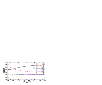
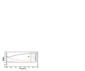
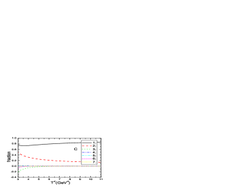
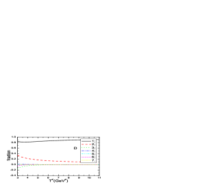
Figure 6: The contributions of different terms in the operator product expansion, the $A$, $B$, $C$ and $D$ correspond to the $D$, $D_{s}$, $B$ and $B_{s}$, respectively; while the 1, 2, 3, 4, 5, 6 and 7 denote the contributions of the perturbative terms, quark condensate, mixed quark condensate, gluon condensate, four-quark condensate $\mathcal{O}(\alpha_{s})$, three-gluon condensate and four-quark condensate $\mathcal{O}(\alpha_{s}^{2})$, respectively.

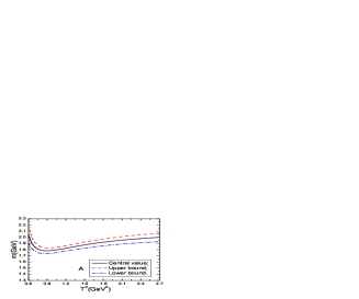
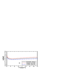
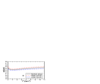
Figure 7: The masses of the heavy pseudoscalar mesons, the $A$, $B$, $C$ and $D$ correspond to the $D$, $D_{s}$, $B$ and $B_{s}$, respectively.

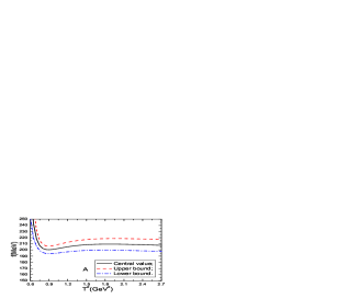
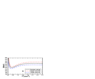
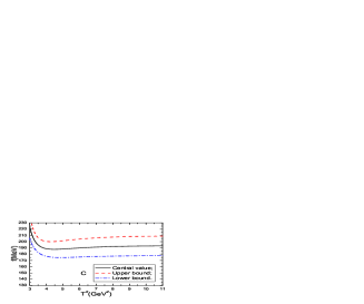
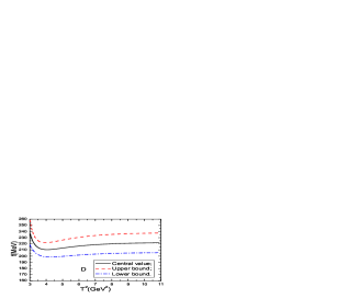
Figure 8: The decay constants of the heavy pseudoscalar mesons, the $A$, $B$, $C$ and $D$ correspond to the $D$, $D_{s}$, $B$ and $B_{s}$, respectively.

In Fig.6, we plot the contributions of different terms in the operator product expansion with variations of the Borel parameters. From the figure, we can see that the convergence of the operator product expansion cannot be satisfied for the $D$ and $D_{s}$ ($B$ and $B_{s}$) mesons at the region $T^{2}<0.9\,\rm{GeV}^{2}$ ($T^{2}<3.0\,\rm{GeV}^{2}$). In Figs.7-8, we plot the masses and decay constants with variations of the Borel parameters at large ranges. Although there appear minimum platforms for the masses and decay constants of the $D$ and $D_{s}$ mesons at $T^{2}\leq 0.9\,\rm{GeV}^{2}$, the Borel windows cannot be chosen in such regions. For the $B$ and $B_{s}$ mesons, the decay constants decrease monotonously with increase of the Borel parameter at $T^{2}<4\,\rm{GeV}^{2}$. We choose the suitable Borel parameters to satisfy the two criteria (pole dominance and convergence of the operator product expansion) of the QCD sum rules, and reproduce the experimental values of the masses. The vacuum condensates play a less important role in the Borel windows, but they play an important role in determining the Borel windows. The threshold parameters, Borel parameters, pole contributions and the resulting decay constants are shown explicitly in Table 1.

In calculations, we observe that the ground state masses are sensitive to the heavy quark $\overline{MS}$ masses, i.e. they increase monotonously with increase of the heavy quark $\overline{MS}$ masses. The $\overline{MS}$ masses from the Particle Data Group happen to result in satisfactory ground state masses compared to the experimental data [9].

In Table 2, we compare the present predictions to the experimental data and some (not all) theoretical calculations. The value $f_{B}=(194\pm 9)\,\rm{MeV}$ listed in the Review of Particle Physics [9] is the average of the lattice QCD calculations [22, 45]. The present predictions $f_{D}=(208\pm 11)\,\rm{MeV}$ and $f_{B}=(189\pm 15)\,\rm{MeV}$ are consistent with the experimental data within uncertainties, while the prediction $f_{D_{s}}=(241\pm 12)\,\rm{MeV}$ is below the lower bound of the experimental data $f_{D_{s}}=(260.0\pm 5.4)\,\rm{MeV}$ [9]. The ratio $f_{D_{s}}/f_{D}\approx f_{B_{s}}/f_{B}$, the heavy quark symmetry works well. In the early work [46], Gershtein and Khlopov obtained a simple relation $f_{ij}\propto m_{i}+m_{j}$ for the decay constant $f_{ij}$ of the pseudoscalar meson having the constituent quarks $i$ and $j$, the simple relation does not work well enough numerically.

Secondly, we study the masses and decay constants of the heavy pseudoscalar mesons in the case of II.

The values of the pole masses listed in the Review of Particle Physics are $m_{c}=(1.67\pm 0.07)\,\rm{GeV}$ and $m_{b}=(4.78\pm 0.06)\,\rm{GeV}$ [9], which correspond to the $\overline{MS}$ masses $m_{c}(m_{c}^{2})=(1.275\pm 0.025)\,\rm{GeV}$ and $m_{b}(m_{b}^{2})=(4.18\pm 0.03)\,\rm{GeV}$, respectively. In calculations, we observe that the heavy pseudoscalar meson masses increase monotonously with increase of the pole masses, the values $m_{c}=1.67\,\rm{GeV}$ and $m_{b}=4.78\,\rm{GeV}$ cannot lead to satisfactory results by choosing reasonable Borel parameters and threshold parameters. We expect that smaller pole masses maybe lead to satisfactory heavy pseudoscalar meson masses, and search for the optimal values.

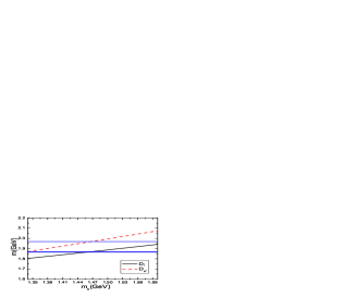
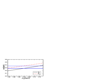
Figure 9: The masses of the heavy pseudoscalar mesons with variations of the pole masses $m_{c}$ and $m_{b}$, where the horizontal lines denote the experimental values.

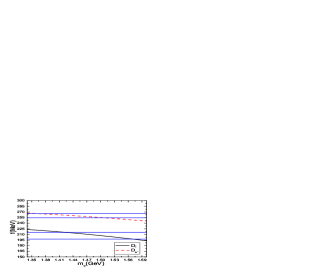
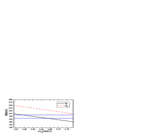
Figure 10: The decay constants of the heavy pseudoscalar mesons with variations of the pole masses $m_{c}$ and $m_{b}$, where the horizontal lines denote the upper and lower bounds of the experimental values.

In Fig.9, we plot the predicted masses with variations of the pole masses with the threshold parameters $s^{0}_{D}=5.5\,\rm{GeV}^{2}$, $s^{0}_{D_{s}}=7.2\,\rm{GeV}^{2}$, $s^{0}_{B}=32.0\,\rm{GeV}^{2}$, $s^{0}_{B_{s}}=34.5\,\rm{GeV}^{2}$ and Borel parameters $T^{2}_{D}=1.7\,\rm{GeV}^{2}$, $T^{2}_{D_{s}}=1.3\,\rm{GeV}^{2}$, $T^{2}_{B}=4.5\,\rm{GeV}^{2}$, $T^{2}_{B_{s}}=4.7\,\rm{GeV}^{2}$ at large ranges. In Fig.10, we plot the corresponding decay constants with variations of the pole masses with the same parameters as in Fig.9. From Fig.9, we can see that the pole masses $m_{c}=1.47\,\rm{GeV}$ and $m_{b}=4.64\,\rm{GeV}$ are the optimal values to reproduce the experimental values of the heavy meson masses. Detailed analysis indicates that those threshold parameters and Borel parameters are also optimal values.

In this article, we take the pole masses as $m_{c}=(1.47\pm 0.06)\,\rm{GeV}$ and $m_{b}=(4.64\pm 0.06)\,\rm{GeV}$, which lead to the uncertainties $\delta m_{D}=\pm 0.03\,\rm{GeV}$, $\delta m_{D_{s}}=\pm 0.05\,\rm{GeV}$, $\delta m_{B}=\pm 0.04\,\rm{GeV}$ and $\delta m_{B_{s}}=\pm 0.04\,\rm{GeV}$. The uncertainties of $\pm(0.03-0.05)\,\rm{GeV}$ are acceptable in the QCD sum rules. In Ref.[13], Penin and Steinhauser take the $b$-quark pole mass as $m_{b}=4.68\,\rm{GeV}$ ($4.78\,\rm{GeV}$), and study the decay constant $f_{B}$ by including perturbative ${\mathcal{O}}(\alpha_{s})$ (${\mathcal{O}}(\alpha_{s}^{2})$) corrections with the QCD sum rules in the heavy quark effective theory, then estimate the $c$-quark pole mass to be $m_{c}=(1.37\pm 0.10)\,\rm{GeV}$. The values of the pole masses $m_{Q}$ from different references overlap with (but not equal to) each other. One may expect to choose larger uncertainties of the pole masses, however, larger $\delta m_{c}$ and $\delta m_{b}$ mean larger derivations from the experimental data $m_{D^{\pm}}=1869.5\,\rm{MeV}$, $m_{D^{0}}=1864.91\,\rm{MeV}$, $m_{D_{s}^{\pm}}=1969.0\,\rm{MeV}$, $m_{B^{\pm}}=5279.25\,\rm{MeV}$, $m_{B^{0}}=5279.55\,\rm{MeV}$ and $m_{B_{s}^{0}}=5366.7\,\rm{MeV}$ [9], see Fig.9. The light quark masses play less important roles, we take the values $m_{u}=m_{d}=0$ and $m_{s}=0.15\,\rm{GeV}$.

Once the pole masses are fixed, we choose suitable Borel parameters and threshold parameters to satisfy the two criteria (pole dominance and convergence of the operator product expansion) of the QCD sum rules, and reproduce the experimental values of the masses. The threshold parameters, Borel parameters, pole contributions and the resulting decay constants are also shown explicitly in Table 1. The resulting decay constants are compared to the experimental data and some (not all) theoretical calculations in Table 2.

From Table 2, we can see that the present predictions $f_{D}=(211\pm 14)\,\rm{MeV}$ and $f_{B}=(190\pm 17)\,\rm{MeV}$ are consistent with the experimental data within uncertainties, while the prediction $f_{D_{s}}=(258\pm 13)\,\rm{MeV}$ is in excellent agreement with the experimental data $f_{D_{s}}=(260.0\pm 5.4)\,\rm{MeV}$ within uncertainties [9]. Furthermore, $f_{D_{s}}/f_{D}\approx f_{B_{s}}/f_{B}$, the heavy quark symmetry works well, the ratio $f_{D_{s}}/f_{D}=1.22\pm 0.08$ is in excellent agreement with the experimental data $f_{D_{s}}/f_{D}=1.26\pm 0.06$ [9]; while most of the theoretical predictions (including the present prediction in the case of I) of the ratio $f_{D_{s}}/f_{D}$ are below the experimental data. We can draw the conclusion tentatively that the prediction $f_{B_{s}}=(233\pm 17)\,\rm{MeV}$ is robust.

In Ref.[16], A. Khodjamirian estimates the upper bound $f_{D}<230\,\rm{MeV}$ and $f_{D_{s}}<270\,\rm{MeV}$ based on the QCD sum rules, the present predictions (both in the cases of I and II) satisfy the constraints. The differences between the predictions in the cases of I and II originate from the systematic uncertainties of the QCD sum rules, we cannot come to the conclusion which predictions are the true values or more close to the true values. The existence of a charged Higgs boson or any other charged object beyond the standard model would modify the decay rates, therefore modify the values of the decay constants, for example, the leptonic decay widths are modified in two-Higgs-doublet models [47]. If the predictions in the case of I are more close to the true values, new physics beyond the standard model are favored so as to smear the discrepancies between the theoretical calculations and experimental data. On the other hand, if the predictions in the case of II are more close to the true values, new physics beyond the standard model are not favored, as the agreements between the experimental data and present theoretical calculations are already excellent.

In the QCD sum rules, the resulting ground state masses are sensitive to the heavy quark masses, variations of the heavy quark masses lead to changes of integral ranges $(m_{Q}+m_{q})^{2}-s_{0}$ of the variable $\rm\bf{ds}$ besides the QCD spectral densities, therefore changes of the Borel windows and predicted masses and decay constants. In this article, we choose both the $\overline{MS}$ masses and pole masses to study the masses and decay constants of the heavy pseudoscalar mesons. We take the following criteria:

$\bullet$ Pole dominance at the phenomenological side;

$\bullet$ Convergence of the operator product expansion;

$\bullet$ Appearance of the Borel platforms;

$\bullet$ Reappearance of experimental values of the ground state heavy meson masses.

The values of the heavy quark $\overline{MS}$ masses from the Particle Data Group can satisfy the four criteria; while the values of the heavy quark pole masses from the Particle Data Group cannot satisfy the four criteria, we choose smaller but reasonable pole masses to satisfy the four criteria. The $\overline{MS}$ masses and pole masses lead to quite different decay constants for the $D_{s}$ and $B_{s}$ mesons. Recently, the Belle collaboration extracted the value,

$$f_{D_{s}} = (255.5\pm 4.2\pm 5.1)\,\rm{MeV}\,,$$ (19)

from the decays $D_{s}^{+}\to\mu^{+}\nu_{\mu}$ and $D_{s}^{+}\to\tau^{+}\nu_{\tau}$ [48], which is in excellent agreement with the present prediction $f_{D_{s}}=(258\pm 13)\,\rm{MeV}$ in the case $\bf\rm II$.

	$T^{2}(\rm{GeV}^{2})$	$s_{0}(\rm{GeV}^{2})$	pole	$m_{P}(\rm{GeV})$	$f_{P}(\rm{MeV})$
$D$ (I)	$1.2-1.8$	$6.2\pm 0.5$	$(66-93)\%$	$1.87\pm 0.10$	$208\pm 11$
$D_{s}$ (I)	$1.2-1.7$	$7.3\pm 0.5$	$(80-96)\%$	$1.97\pm 0.10$	$241\pm 12$
$B$ (I)	$4.7-6.1$	$33.5\pm 1.0$	$(46-70)\%$	$5.28\pm 0.06$	$189\pm 15$
$B_{s}$ (I)	$5.1-6.6$	$35.0\pm 1.0$	$(47-71)\%$	$5.37\pm 0.06$	$216\pm 16$
$D$ (II)	$1.4-2.0$	$5.5\pm 0.5$	$(54-84)\%$	$1.87\pm 0.06$	$211\pm 14$
$D_{s}$ (II)	$1.0-1.6$	$7.2\pm 0.5$	$(84-99)\%$	$1.97\pm 0.08$	$258\pm 13$
$B$ (II)	$4.1-4.9$	$32.0\pm 1.0$	$(51-71)\%$	$5.28\pm 0.06$	$190\pm 17$
$B_{s}$ (II)	$4.3-5.1$	$34.5\pm 1.0$	$(61-79)\%$	$5.37\pm 0.05$	$233\pm 17$

Table 1: The Borel parameters, continuum threshold parameters, pole contributions, masses and decay constants for the heavy pseudoscalar mesons.

	$f_{D}(\rm{MeV})$	$f_{D_{s}}(\rm{MeV})$	$f_{B}(\rm{MeV})$	$f_{B_{s}}(\rm{MeV})$	$f_{D_{s}}/f_{D}$	$f_{B_{s}}/f_{B}$
Expt [9]	$206.7\pm 8.9$	$260.0\pm 5.4$	$194\pm 9$		$1.26\pm 0.06$
QCDSR [13]	$195\pm 20$		$206\pm 20$
QCDSR [14]	$177\pm 21$	$205\pm 22$	$178\pm 14$	$200\pm 14$	$1.16\pm 0.16$	$1.12\pm 0.11$
QCDSR [17]	$206.2\pm 7.3$	$245.3\pm 15.7$	$193.4\pm 12.3$	$232.5\pm 18.6$	$1.193\pm 0.025$	$1.203\pm 0.020$
QCDSR [18]	$204\pm 6$	$246\pm 6$	$207\pm 8$	$234\pm 5$	$1.21\pm 0.04$	$1.14\pm 0.03$
LQCD [20]	$197\pm 9$	$244\pm 8$			$1.24\pm 0.03$
LQCD [21]	$213\pm 4$	$248.0\pm 2.5$	$191\pm 9$	$228\pm 10$	$1.164\pm 0.018$	$1.188\pm 0.018$
LQCD [22]	$218.9\pm 11.3$	$260.1\pm 10.8$	$196.9\pm 8.9$	$242.0\pm 9.5$	$1.188\pm 0.025$	$1.229\pm 0.026$
BSE [23]	$238$	$241$	$193$	$195$	$1.01$	$1.01$
RPM [26]	$234$	$268$	$189$	$218$	$1.15$	$1.15$
FCM [28]	$210\pm 10$	$260\pm 10$	$182\pm 8$	$216\pm 8$	$1.24\pm 0.03$	$1.19\pm 0.02$
LFQM[30]	$205.8\pm 8.9$	$264.5\pm 17.5$	$204\pm 31$	$270.0\pm 42.8$	$1.29\pm 0.07$	$1.32\pm 0.08$
This work (I)	$208\pm 11$	$241\pm 12$	$189\pm 15$	$216\pm 16$	$1.16\pm 0.07$	$1.14\pm 0.11$
This work (II)	$211\pm 14$	$258\pm 13$	$190\pm 17$	$233\pm 17$	$1.22\pm 0.08$	$1.23\pm 0.12$

Table 2: The decay constants of the heavy pseudoscalar mesons from the experimental data and some theoretical calculations.

4 Conclusion

In this article, we recalculate the contributions of all vacuum condensates up to dimension-6, in particular the one-loop corrections to the quark condensates $\alpha_{s}\langle\bar{q}q\rangle$ and partial one-loop corrections to the four-quark condensates $\alpha_{s}^{2}\langle\bar{q}q\rangle^{2}$, in the operator product expansion, and obtain the analytical QCD spectral densities. Then we study the masses and decay constants of the heavy pseudoscalar mesons using the QCD sum rules with the two possible choices: I we choose the $\overline{MS}$ masses by setting $m=m(\mu)$ and take perturbative corrections up to the order $\mathcal{O}(\alpha_{s})$; II we choose the pole masses $m$, take perturbative corrections up to the order $\mathcal{O}(\alpha_{s}^{2})$ and set the energy-scale $\mu=m_{Q}$. In the case of I, the predictions $f_{D}=(208\pm 11)\,\rm{MeV}$ and $f_{B}=(189\pm 15)\,\rm{MeV}$ are consistent with the experimental data within uncertainties, while the prediction $f_{D_{s}}=(241\pm 12)\,\rm{MeV}$ is still below the lower bound of the experimental data $f_{D_{s}}=(260.0\pm 5.4)\,\rm{MeV}$, new physics beyond the standard model are favored so as to smear the discrepancies, in other words, there are rooms for new physics to smear the discrepancies. In the case of II, the predictions $f_{D}=(211\pm 14)\,\rm{MeV}$, $f_{B}=(190\pm 17)\,\rm{MeV}$, $f_{D_{s}}=(258\pm 13)\,\rm{MeV}$ and $f_{D_{s}}/f_{D}=1.22\pm 0.08$ are all in excellent agreements with the experimental data within uncertainties, new physics beyond the standard model are not favored, in other words, the new physics models should satisfy more stringent constraints. The differences between the predictions in the cases of I and II originate from the systematic uncertainties of the QCD sum rules, we cannot come to the conclusion which predictions are the true values or more close to the true values.

References

- [1] G. Bonvicini, Phys. Rev. D70 (2004) 112004.
- [2] M. Artuso et al, Phys. Rev. Lett. 95 (2005) 251801.
- [3] B. I. Eisenstein et al, Phys. Rev. D78 (2008) 052003.
- [4] J. P. Alexander, Phys. Rev. D79 (2009) 052001.
- [5] P. U. E. Onyisi et al, Phys. Rev. D79 (2009) 052002.
- [6] P. Naik et al, Phys. Rev. D80 (2009) 112004.
- [7] P. del Amo Sanchez et al, Phys. Rev. D82 (2010) 091103.
- [8] L. Widhalm et al, Phys. Rev. Lett. 100 (2008) 241801.
- [9] J. Beringer et al, Phys. Rev. D86 (2012) 010001.
- [10] T. M. Aliev and V. L. Eletsky, Sov. J. Nucl. Phys. 38 (1983) 936.
- [11] C. A. Dominguez and N. Paver, Phys. Lett. B197 (1987) 423; S. Narison, Phys. Lett. B198 (1987) 104; L. J. Reinders, Phys. Rev. D38 (1988) 947; M. Jamin and M. Munz, Z. Phys. C60 (1993) 569; S. Narison, Phys. Lett. B520 (2001) 115; M. Jamin and B. O. Lange, Phys. Rev. D65 (2002) 056005; H. Y. Jin, J. Zhang and Z. F. Zhang, Phys. Rev. D81 (2010) 054021.
- [12] K. G. Chetyrkin and M. Steinhauser, Phys. Lett. B502 (2001) 104; K. G. Chetyrkin and M. Steinhauser, Eur. Phys. J. C21 (2001) 319.
- [13] A. A. Penin and M. Steinhauser, Phys. Rev. D65 (2002) 054006.
- [14] J. Bordes, J. Penarrocha and K. Schilcher, JHEP 0412 (2004) 064; J. Bordes, J. Penarrocha and K. Schilcher, JHEP 0511 (2005) 014.
- [15] S. Narison, Phys. Lett. B668 (2008) 308.
- [16] A. Khodjamirian, Phys. Rev. D79 (2009) 031503.
- [17] W. Lucha, D. Melikhov and S. Simula, Phys. Lett. B701 (2011) 82; W. Lucha, D. Melikhov and S. Simula, J. Phys. G38 (2011) 105002.
- [18] S. Narison, Phys. Lett. B718 (2013) 1321.
- [19] A. X. El-Khadra et al, Phys. Rev. D58 (1998) 014506; D. Becirevic et al, Phys. Rev. D60 (1999) 074501; S. Collins et al, Phys. Rev. D63 (2001) 034505; K. C. Bowler et al, Nucl. Phys. B619 (2001) 507; G. M. de Divitiis et al, Nucl. Phys. B672 (2003) 372; A. Gray et al, Phys. Rev. Lett. 95 (2005) 212001; C. Bernard et al, PoS LATTICE2008 (2008) 278; E. T. Neil et al, PoS LATTICE2011 (2011) 320; D. Becirevic et al, JHEP 1202 (2012) 042.
- [20] B. Blossier et al, JHEP 0907 (2009) 043.
- [21] C. T. H. Davies et al, Phys. Rev. D82 (2010) 114504; H. Na et al, Phys. Rev. D86 (2012) 034506.
- [22] A. Bazavov et al, Phys. Rev. D85 (2012) 114506.
- [23] Z. G. Wang, W. M. Yang and S. L. Wan, Nucl. Phys. A744 (2004) 156.
- [24] G. Cvetic, C. S. Kim, G. L. Wang and W. Namgung, Phys. Lett. B596 (2004) 84.
- [25] P. Colangelo, G. Nardulli and M. Pietroni, Phys. Rev. D43 (1991) 3002.
- [26] D. Ebert, R. N. Faustov and V. O. Galkin, Phys. Lett. B635 (2006) 93.
- [27] M. Z. Yang, Eur. Phys. J. C72 (2012) 1880.
- [28] A. M. Badalian, B. L. G. Bakker and Yu. A. Simonov, Phys. Rev. D75 (2007) 116001.
- [29] H. M. Choi, Phys. Rev. D75 (2007) 073016.
- [30] C. W. Hwang, Phys. Rev. D81 (2010) 114024.
- [31] X. H. Guo and M. H. Weng, Eur. Phys. J. C50 (2007) 63.
- [32] D. Ebert, T. Feldmann, R. Friedrich and H. Reinhardt, Nucl. Phys. B434 (1995) 619; S. Nam, Phys. Rev. D85 (2012) 034019.
- [33] A. Hayashigaki and K. Terasaki, hep-ph/0411285.
- [34] M. A. Shifman, A. I. Vainshtein and V. I. Zakharov, Nucl. Phys. B147 (1979) 385.
- [35] L. J. Reinders, H. Rubinstein and S. Yazaki, Phys. Rept. 127 (1985) 1.
- [36] P. del Amo Sanchez et al, Phys. Rev. D82 (2010) 111101.
- [37] Z. G. Wang, Phys. Rev. D83 (2011) 014009; B. Chen, L. Yuan and A. Zhang, Phys. Rev. D83 (2011) 114025; A. M. Badalian and B. L. G. Bakker, Phys. Rev. D84 (2011) 034006; P. Colangelo, F. De Fazio, F. Giannuzzi and S. Nicotri, Phys. Rev. D86 (2012) 054024.
- [38] A. Hoell, A. Krassnigg, C. D. Roberts and S. V. Wright, Int. J. Mod. Phys. A20 (2005) 1778.
- [39] C. McNeile and C. Michael, Phys. Lett. B642 (2006) 244.
- [40] K. Maltman and J. Kambor, Phys. Rev. D65 (2002) 074013.
- [41] M. Diehl and G. Hiller, JHEP 06 (2001) 067.
- [42] P. Colangelo and A. Khodjamirian, hep-ph/0010175; B. L. Ioffe, Prog. Part. Nucl. Phys. 56 (2006) 232.
- [43] S. Narison, Camb. Monogr. Part. Phys. Nucl. Phys. Cosmol. 17 (2002) 1.
- [44] S. Narison, Phys. Lett. B693 (2010) 559; S. Narison, Phys. Lett. B706 (2012) 412; S. Narison, Phys. Lett. B707 (2012) 259.
- [45] E. Gamiz et al, Phys. Rev. D80 (2009) 014503.
- [46] S. S. Gershtein, M. Yu. Khlopov, JETP Lett. 23 (1976) 338; M. Yu. Khlopov, Sov. J. Nucl. Phys. 28 (1978) 583.
- [47] A. G. Akeroyd and C. H. Chen, Phys. Rev. D75 (2007) 075004; A. G. Akeroyd and F. Mahmoudi, JHEP 0904 (2009) 121.
- [48] A. Zupanc et al, arXiv:1307.6240.