Object-oriented implementations of the MPDATA advection equation solver in C++, Python and Fortran

Abstract

Three object-oriented implementations of a prototype solver of the advection equation are introduced. The presented programs are based on Blitz++ (C++), NumPy (Python), and Fortran’s built-in array containers. The solvers include an implementation of the Multidimensional Positive-Definite Advective Transport Algorithm (MPDATA). The introduced codes exemplify how the application of object-oriented programming (OOP) techniques allows to reproduce the mathematical notation used in the literature within the program code. A discussion on the tradeoffs of the programming language choice is presented. The main angles of comparison are code brevity and syntax clarity (and hence maintainability and auditability) as well as performance. In the case of Python, a significant performance gain is observed when switching from the standard interpreter (CPython) to the PyPy implementation of Python. Entire source code of all three implementations is embedded in the text and is licensed under the terms of the GNU GPL license.

1 Introduction

Object oriented programming (OOP) ”has become recognised as the almost unique successful paradigm for creating complex software” [1, Sec. 1.3]. It is intriguing that, while the quoted statement comes from the very book subtitled The Art of Scientific Computing, hardly any (if not none) of the currently operational weather and climate prediction systems - flagship examples of complex scientific software - make extensive use of OOP techniques. Fortran has been the language of choice in oceanic [2], weather-prediction [3] and Earth system [4] modelling, and none of its 20-century editions were object-oriented languages [see e.g. 5, for discussion].

Application of OOP techniques in development of numerical modelling software may help to:

1. maintain modularity and separation of program logic layers (e.g. separation of numerical algorithms, parallelisation mechanisms, data input/output, error handling and the description of physical processes); and

2. shorten and simplify the source code and improve its readability by reproducing within the program logic the mathematical notation used in the literature.

The first application is attainable, yet arguably cumbersome, with procedural programming. The latter, virtually impossible to obtain with procedural programming, is the focus of this paper. It also enables the compiler or library authors to relieve the user (i.e. scientific programmer) from hand-coding optimisations, a practice long recognised as having a strong negative impact when debugging and maintenance are considered [6].

MPDATA [7] stands for Multidimensional Positive Definite Advective Transport Algorithm and is an example of a numerical procedure used in weather, climate and ocean simulation systems [e.g. 8, 9, 10, respectively]. MPDATA is a solver for systems of advection equations of the following form:

$$\partial_{t}\psi=-\nabla\cdot(\vec{v}\psi)$$ (1)

that describe evolution of a scalar field $\psi$ transported by the fluid flow with velocity $\vec{v}$. Quoting Numerical Recipes once more, development of methods to numerically solve such problems ”is an art as much as a science” [1, Sec. 20.1], and MPDATA is an example of the state-of-the art in this field. MPDATA is designed to accurately solve equation (1) in an arbitrary number of dimensions assuring positive-definiteness of scalar field $\psi$ and incurring small numerical diffusion. All relevant MPDATA formulæ are given in the text but are presented without derivation or detailed discussion. For a recent review of MPDATA-based techniques see Smolarkiewicz [11, and references therein].

In this paper we introduce and discuss object-oriented implementations of an MPDATA-based two-dimensional (2D) advection equation solver written in C++11 (ISO/IEC 14882:2011), Python [13] and Fortran 2008 (ISO/IEC 1539-1:2010). In the following section we introduce the three implementations briefly describing the algorithm itself and discussing where and how the OOP techniques may be applied in its implementation. The syntax and nomenclature of OOP techniques are used without introduction, for an overview of OOP in context of C++, Python and Fortran, consult for example [15, Part II], [16, Chapter 5] and [17, Chapter 11], respectively. The third section of this paper covers performance evaluation of the three implementations. The fourth section covers discussion of the tradeoffs of the programming language choice. The fifth section closes the article with a brief summary.

Throughout the paper we present the three implementations by discussing source code listings which cover the entire program code. Subsections 2.1-2.6 describe all three implementations, while subsequent sections 2.7-2.12 cover discussion of C++ code only. The relevant parts of Python and Fortran codes do not differ significantly, and for readability reasons are presented in P and F, respectively.

The entire code is licensed under the terms of the GNU General Public License license version 3 [18].

All listings include line numbers printed to the left of the source code, with separate numbering for C++ (listings prefixed with C, black frame),

  listing C.0 (C++)     1 // code licensed under the terms of GNU GPL v3 2 // copyright holder: University of Warsaw      Python (listings prefixed with P, blue frame) and

  listing P.0 (Python)     1 # code licensed under the terms of GNU GPL v3 2 # copyright holder: University of Warsaw      Fortran (listings prefixed with F, red frame).

  listing F.0 (Fortran)     1 ! code licensed under the terms of GNU GPL v3 2 ! copyright holder: University of Warsaw      Programming language constructs when inlined in the text are typeset in bold, e.g. GOTO 2.

2 Implementation

Double precision floating-point format is used in all three implementations. The codes begin with the following definitions:

  listing C.1 (C++)     3 typedef double real_t;     

  listing P.1 (Python)     3 real_t = ’float64’     

  listing F.1 (Fortran)     3 module real_m 4   implicit none 5   integer, parameter :: real_t = kind(0.d0) 6 end module      which provide a convenient way of switching to different precision.

All codes are structured in a way allowing compilation of the code in exactly the same order as presented in the text within one source file, hence every Fortran listing contains definition of a separate module.

2.1 Array containers

Solution of equation (1) using MPDATA implies discretisation onto a grid of the $\psi$ and the Courant number $\vec{C}=\vec{v}\cdot\frac{\Delta t}{\Delta x}$ fields, where $\Delta t$ is the solver timestep and $\Delta x$ is the grid spacing.

Presented C++ implementation of MPDATA is built upon the Blitz++ library. Blitz offers object-oriented representation of n-dimensional arrays, and array-valued mathematical expressions. In particular, it offers loop-free notation for array arithmetics that does not incur creation of intermediate temporary objects. Blitz++ is a header-only library – to use it, it is enough to include the appropriate header file, and optionally expose the required classes to the present namespace:

  listing C.2 (C++)     4 #include <blitz/array.h> 5 using arr_t = blitz::Array<real_t, 2>; 6 using rng_t = blitz::Range; 7 using idx_t = blitz::RectDomain<2>;      Here arr_t, rng_t and idx_t serve as alias identifiers and are introduced in order to shorten the code.

The power of Blitz++ comes from the ability to express array expressions as objects. In particular, it is possible to define a function that returns an array expression; i.e. not the resultant array, but an object representing a ,,recipe” defining the operations to be performed on the arguments. As a consequence, the return types of such functions become unintelligible. Luckily, the auto return type declaration from the C++11 standard allows to simplify the code significantly, even more if used through the following preprocessor macro:

  listing C.3 (C++)     8 #define return_macro(expr) \ 9   -> decltype(safeToReturn(expr)) \ 10 { return safeToReturn(expr); }       The call to blitz::safeToReturn() function is included in order to ensure that all arrays involved in the expression being returned continue to exist in the caller scope. For example, definition of a function returning its array-valued argument doubled, reads: auto f(arr_t x) return_macro(2*x). This is the only preprocessor macro defined herein.

For the Python implementation of MPDATA the NumPy package is used. In order to make the code compatible with both the standard CPython as well as the alternative PyPy implementation of Python [19], the Python code includes the following sequence of import statements:

  listing P.2 (Python)     4 try: 5   import numpypy 6   from _numpypy.pypy import set_invalidation 7   set_invalidation(False) 8 except ImportError: 9   pass 10 import numpy 11 try: 12   numpy.seterr(all=’ignore’) 13 except AttributeError: 14   pass      First, the PyPy’s built-in NumPy implementation named numpypy is imported if applicable (i.e. if running PyPy), and the lazy evaluation mode is turned on through the set_invalidation(False) call. PyPy’s lazy evaluation obtained with the help of a just-in-time compiler enables to achieve an analogous to Blitz++ temporary-array-free handling of array-valued expressions (see discussion in section 3). Second, to match the settings of C++ and Fortran compilers used herein, the NumPy package is instructed to ignore any floating-point errors, if such an option is available in the interpreter. The above lines conclude all code modifications that needed to be added in order to run the code with PyPy.

Among the three considered languages only Fortran is equipped with built-in array handling facilities of practical use in high-performance computing. Therefore, there is no need for using an external package as with C++ and Python. Fortran array-handling features are not object-oriented, though.

2.2 Containers for sequences of arrays

As discussed above, discretisation in space of the scalar field $\psi(x,y)$ into its $\psi_{[i,j]}$ grid representation requires floating-point array containers. In turn, discretisation in time requires a container class for storing sequences of such arrays, i.e. {$\psi^{[n]}$, $\psi^{[n+1]}$}. Similarly the components of the vector field $\vec{C}$ are in fact a {$C^{[x]}$, $C^{[y]}$} array sequence.

Using an additional array dimension to represent the sequence elements is not considered for two reasons. First, the $C^{[x]}$ and $C^{[y]}$ arrays constituting the sequence have different sizes (see discussion of the Arakawa-C grid in section 2.3). Second, the order of dimensions would need to be different for different languages to assure that the contiguous dimension is used for one of the space dimensions and not for time levels.

In the C++ implementation the Boost ptr_vector class is used to represent sequences of Blitz++ arrays and at the same time to handle automatic freeing of dynamically allocated memory. The ptr_vector class is further customised by defining a derived structure which element-access [ ] operator is overloaded with a modulo variant:

  listing C.4 (C++)     11 #include <boost/ptr_container/ptr_vector.hpp> 12 struct arrvec_t : boost::ptr_vector<arr_t> 13 { 14   const arr_t &operator[](const int i) const 15   { 16     return this->at((i + this->size()) % this->size()); 17   } 18 };      Consequently the last element of any such sequence may be accessed at index -1, the last but one at -2, and so on.

In the Python implementation the built-in tuple type is used to store sequences of NumPy arrays. Employment of negative indices for handling from-the-end addressing of elements is a built-in feature of all sequence containers in Python.

Fortran does not feature any built-in sequence container capable of storing arrays, hence a custom arrvec_t type is introduced:

  listing F.2 (Fortran)     7 module arrvec_m 8   use real_m 9   implicit none 10  11   type :: arr_t 12     real(real_t), allocatable :: a(:,:) 13   end type 14  15   type :: arrptr_t 16     class(arr_t), pointer :: p 17   end type 18  19   type :: arrvec_t 20     class(arr_t), allocatable :: arrs(:) 21     class(arrptr_t), allocatable :: at(:) 22     integer :: length 23     contains 24     procedure :: ctor => arrvec_ctor 25     procedure :: init => arrvec_init 26   end type 27  28   contains 29  30   subroutine arrvec_ctor(this, n) 31     class(arrvec_t) :: this 32     integer, intent(in) :: n 33  34     this%length = n 35     allocate(this%at( -n : n-1 )) 36     allocate(this%arrs( 0 : n-1 )) 37   end subroutine 38  39   subroutine arrvec_init(this, n, i, j) 40     class(arrvec_t), target :: this 41     integer, intent(in) :: n 42     integer, intent(in) :: i(2), j(2) 43  44     allocate(this%arrs(n)%a( i(1) : i(2), j(1) : j(2) )) 45     this%at(n)%p => this%arrs(n) 46     this%at(n - this%length)%p => this%arrs(n) 47   end subroutine 48 end module      The arr_t type is defined solely for the purpose of overcoming the limitation of lack of an array-of-arrays construct, and its only member field is a two-dimensional array. An array of arr_t is used hereinafter as a container for sequences of arrays.

The arrptr_t type is defined solely for the purpose of overcoming Fortran’s limitation of not supporting allocatables of pointers. arrptr_t’s single member field is a pointer to an instance of arr_t. Creating an allocatable of arrptr_t, instead of a multi-element pointer of arr_t, ensures automatic memory deallocation.

Type arrptr_t is used to implement the from-the-end addressing of elements in arrvec_t. The array data is stored in the arrs member field (of type arr_t). The at member field (of type arrptr_t) stores pointers to the elements of arrs. at has double the length of arrs and is initialised in a cyclic manner so that the -1 element of at points to the last element of arrs, and so on. Assuming psi is an instance of arrptr_t, the (i,j) element of the n-th array in psi may be accessed with
psi%at( n )%p%a( i, j ).

The ctor(n) method initialises the container for a given number of elements n. The init(n,i,j) method initialises the n-th element of the container with a newly allocated 2D array spanning indices i(1):i(2), and j(1):j(2) in the first, and last dimensions respectively.

2.3 Staggered grid

Figure 1: A schematic of the Arakawa-C grid.

The so-called Arakawa-C staggered grid [20] depicted in Figure 1 is a natural choice for MPDATA. As a consequence, the discretised representations of the $\psi$ scalar field, and each component of the ${\vec{C}=\vec{v}\cdot\frac{\Delta t}{\Delta x}}$ vector field in eq. (1) are defined over different grid point locations. In mathematical notation this can be indicated by usage of fractional indices, e.g. $C^{[x]}_{[i\scalebox{0.4}[0.8]{$-$}\nicefrac{{1}}{{2}},j]}$, $C^{[x]}_{[i+\nicefrac{{1}}{{2}},j]}$, $C^{[y]}_{[i,j\scalebox{0.4}[0.8]{$-$}\nicefrac{{1}}{{2}}]}$ and $C^{[y]}_{[i,j+\nicefrac{{1}}{{2}}]}$ to depict the grid values of the ${\vec{C}}$ vector components surrounding $\psi_{[i,j]}$. However, fractional indexing does not have a built-in counterpart in any of the employed programming languages. A desired syntax would translate $i-\nicefrac{{1}}{{2}}$ to $i-1$ and $i+\nicefrac{{1}}{{2}}$ to $i$. OOP offers a convenient way to implement such notation by overloading the + and - operators for objects representing array indices.

In the C++ implementation first a global instance h of an empty structure hlf_t is defined, and then the plus and minus operators for hlf_t and rng_t are overloaded:

  listing C.5 (C++)     19 struct hlf_t {} h; 20  21 inline rng_t operator+(const rng_t &i, const hlf_t &) 22 { 23   return i; 24 } 25  26 inline rng_t operator-(const rng_t &i, const hlf_t &) 27 { 28   return i-1; 29 }      This way, the arrays representing vector field components can be indexed using (i+h,j), (i-h,j) etc. where h represents the half.

In NumPy in order to prevent copying of array data during slicing one needs to operate on the so-called array views. Array views are obtained when indexing the arrays with objects of the Python’s built-it slice type (or tuples of such objects in case of multi-dimensional arrays). Python forbids overloading of operators of built-in types such as slices, and does not define addition/subtraction operators for slice and int pairs. Consequently, a custom logic has to be defined not only for fractional indexing, but also for shifting the slices by integer intervals ($i\pm 1$). It is implemented here by declaring a shift class with the adequate operator overloads:

  listing P.3 (Python)     15 class shift(): 16   def __init__(self, plus, mnus): 17     self.plus = plus 18     self.mnus = mnus 19   def __radd__(self, arg): 20     return type(arg)( 21       arg.start + self.plus, 22       arg.stop  + self.plus 23     ) 24   def __rsub__(self, arg): 25     return type(arg)( 26       arg.start - self.mnus, 27       arg.stop  - self.mnus 28     )      and two instances of it to represent unity and half in expressions like i+one, i+hlf, where i is an instance of slice :

  listing P.4 (Python)     29 one = shift(1,1) 30 hlf = shift(0,1)     

In Fortran fractional array indexing is obtained through definition and instantiation of an object representing the half, and having appropriate operator overloads:

  listing F.3 (Fortran)     49 module arakawa_c_m 50   implicit none 51  52   type :: half_t 53   end type 54  55   type(half_t) :: h 56  57   interface operator (+) 58     module procedure ph 59   end interface 60  61   interface operator (-) 62     module procedure mh 63   end interface 64  65   contains 66  67   elemental function ph(i, h) result (return) 68     integer, intent(in) :: i 69     type(half_t), intent(in) :: h 70     integer :: return 71     return = i 72   end function 73  74   elemental function mh(i, h) result (return) 75     integer, intent(in) :: i 76     type(half_t), intent(in) :: h 77     integer :: return 78     return = i - 1 79   end function 80 end module     

2.4 Halo regions

The MPDATA formulæ defining $\psi^{[n+1]}_{[i,j]}$ as a function of $\psi^{[n]}_{[i,j]}$ (discussed in the following sections) feature terms such as $\psi_{[i-1,j-1]}$. One way of assuring validity of these formulæ on the edges of the domain (e.g. for i=0) is to introduce the so-called halo region surrounding the domain. The method of populating the halo region with data depends on the boundary condition type. Employment of the halo-region logic implies repeated usage of array range extensions in the code such as $i\leadsto i\pm halo$.

An ext() function is defined in all three implementation, in order to simplify coding of array range extensions:

  listing C.6 (C++)     30 template<class n_t> 31 inline rng_t ext(const rng_t &r, const n_t &n) { 32   return rng_t( 33     (r - n).first(), 34     (r + n).last() 35   ); 36 }     

  listing P.5 (Python)     31 def ext(r, n): 32   if (type(n) == int) & (n == 1): 33     n = one 34   return slice( 35     (r - n).start, 36     (r + n).stop 37   )     

  listing F.4 (Fortran)     81 module halo_m 82   use arakawa_c_m 83   implicit none 84  85   interface ext 86     module procedure ext_n 87     module procedure ext_h 88   end interface  89  90   contains 91  92   function ext_n(r, n) result (return) 93     integer, intent(in) :: r(2) 94     integer, intent(in) :: n 95     integer :: return(2) 96  97     return = (/ r(1) - n, r(2) + n /) 98   end function 99  100   function ext_h(r, h) result (return) 101     integer, intent(in) :: r(2) 102     type(half_t), intent(in) :: h 103     integer :: return(2) 104  105     return = (/ r(1) - h, r(2) + h /) 106   end function 107 end module      Consequently, a range depicted by $i\pm 1/2$ may be expressed in the code as ext(i, h). In all three implementations the ext() function accept the second argument to be an integer or a ”half” (cf. section 2.3).

2.5 Array index permutations

Hereinafter, the $\pi_{a,b}^{d}$ symbol is used to denote a cyclic permutation of an order $d$ of a set $\{a,b\}$. It is used to generalise the MPDATA formulæ into multiple dimensions using the following notation:

$$\sum\limits_{d=0}^{1}\psi_{[i,j]+\pi_{1,0}^{d}}\equiv\psi_{[i+1,j]}+\psi_{[i,j+1]}$$

Blitz++ ships with the RectDomain class (aliased here as idx_t) for specifying array ranges in multiple dimensions. The $\pi$ permutation is implemented in C++ as a function pi() returning an instance of idx_t. In order to ensure compile-time evaluation, the permutation order is passed via the template parameter d (note the different order of i and j arguments in the two template specialisations):

  listing C.7 (C++)     37 template<int d> 38 inline idx_t pi(const rng_t &i, const rng_t &j); 39  40 template<> 41 inline idx_t pi<0>(const rng_t &i, const rng_t &j) 42 { 43   return idx_t({i,j}); 44 }; 45  46 template<> 47 inline idx_t pi<1>(const rng_t &j, const rng_t &i) 48 { 49   return idx_t({i,j}); 50 };     

NumPy uses tuples of slices for addressing multi-dimensional array with a single object. Therefore, the following definition of function pi() suffices to represent $\pi$:

  listing P.6 (Python)     38 def pi(d, *idx): 39   return (idx[d], idx[d-1])     

In the Fortran implementation pi() returns a pointer to the array elements specified by i and j interpreted as (i,j) or (j,i) depending on the value of the argument d. In addition to pi(), a helper span() function returning the length of one of the vectors passed as argument is defined:

  listing F.5 (Fortran)     108 module pi_m 109   use real_m 110   implicit none 111   contains 112   function pi(d, arr, i, j) result(return) 113     integer, intent(in) :: d 114     real(real_t), allocatable, target :: arr(:,:) 115     real(real_t), pointer :: return(:,:) 116     integer, intent(in) :: i(2), j(2) 117     select case (d) 118       case (0) 119         return => arr( i(1) : i(2), j(1) : j(2) ) 120       case (1) 121         return => arr( j(1) : j(2), i(1) : i(2) ) 122     end select 123   end function 124  125   pure function span(d, i, j) result(return) 126     integer, intent(in) :: i(2), j(2) 127     integer, intent(in) :: d 128     integer :: return 129     select case (d) 130       case (0) 131         return = i(2) - i(1) + 1 132       case (1) 133         return = j(2) - j(1) + 1 134     end select 135   end function 136 end module      The span() function is used to shorten the declarations of arrays to be returned from functions in the Fortran implementation (see listings F.11 and F.17–F.20).

It is worth noting here that the C++ implementation of pi() is branchless thanks to employment of template specialisation. With Fortran one needs to rely on compiler optimisations to eliminate the conditional expression within the pi() that depends on value of d which is always known at compile time.

2.6 Prototype solver

The tasks to be handled by a prototype advection equation solver proposed herein are:

1. storing arrays representing the $\psi$ and $\vec{C}$ fields and any required housekeeping data,

2. allocating and deallocating the required memory,

3. providing access to the solver state,

4. performing the integration by invoking the advection-operator and boundary-condition handling routines.

In the following C++ definition of the solver structure, task (i) is represented with the definition of the structure member fields; task (ii) is split between the solver’s constructor and the destructors of arrvec_t; task (iii) is handled by the accessor methods; task (iv) is handled within the solve method:

  listing C.8 (C++)     51 template<class bcx_t, class bcy_t> 52 struct solver 53 { 54   // member fields 55   arrvec_t psi, C; 56   int n, hlo; 57   rng_t i, j; 58   bcx_t bcx; 59   bcy_t bcy; 60  61   // ctor 62   solver(int nx, int ny, int hlo) : 63     hlo(hlo), 64     n(0), 65     i(0, nx-1), 66     j(0, ny-1), 67     bcx(i, j, hlo), 68     bcy(j, i, hlo) 69   { 70     for (int l = 0; l < 2; ++l) 71       psi.push_back(new arr_t(ext(i, hlo), ext(j, hlo))); 72     C.push_back(new arr_t(ext(i, h), ext(j, hlo))); 73     C.push_back(new arr_t(ext(i, hlo), ext(j, h))); 74   } 75  76   // accessor methods 77   arr_t state() { 78     return psi[n](i,j).reindex({0,0}); 79   } 80  81   arr_t courant(int d) 82   { 83     return C[d]; 84   } 85  86   // helper methods invoked by solve() 87   virtual void advop() = 0; 88  89   void cycle() 90   { 91     n = (n + 1) % 2 - 2; 92   } 93  94   // integration logic 95   void solve(const int nt) 96   { 97     for (int t = 0; t < nt; ++t) 98     { 99       bcx.fill_halos(psi[n], ext(j, hlo)); 100       bcy.fill_halos(psi[n], ext(i, hlo)); 101       advop(); 102       cycle(); 103     } 104   } 105 };      The solver structure is an abstract definition (containing a pure virtual method) requiring its descendants to implement at least the advop() method which is expected to fill psi[n+1] with an updated (advected) values of psi[n]. The two template parameters bcx_t and bcy_t allow the solver to operate with any kind of boundary condition structures that fulfil the requirements implied by the calls to the methods of bcx and bcy, respectively.

The donor-cell and MPDATA schemes both require only the previous state of an advected field in order to advance the solution. Consequently, memory for two time levels ($\psi^{[n]}$ and $\psi^{[n+1]}$) is allocated in the constructor. The sizes of the arrays representing the two time levels of $\psi$ are defined by the domain size (nx$~{}\times$ ny) plus the halo region. The size of the halo region is an argument of the constructor. The cycle() method is used to swap the time levels without copying any data.

The arrays representing the $C^{[x]}$ and $C^{[y]}$ components of $\vec{C}$, require (nx+1) $\times$ ny and nx$~{}\times$ (ny+1) elements, respectively (being laid out on the Arakawa-C staggered grid).

Python definition of the solver class follows closely the C++ structure definition:

  listing P.7 (Python)     40 class solver(object): 41   # ctor-like method 42   def __init__(self, bcx, bcy, nx, ny, hlo): 43     self.n = 0 44     self.hlo = hlo 45     self.i = slice(hlo, nx + hlo) 46     self.j = slice(hlo, ny + hlo) 47  48     self.bcx = bcx(0, self.i, hlo) 49     self.bcy = bcy(1, self.j, hlo) 50  51     self.psi = ( 52       numpy.empty(( 53         ext(self.i, self.hlo).stop, 54         ext(self.j, self.hlo).stop 55       ), real_t), 56       numpy.empty(( 57         ext(self.i, self.hlo).stop, 58         ext(self.j, self.hlo).stop 59       ), real_t) 60     ) 61  62     self.C = ( 63       numpy.empty(( 64         ext(self.i, hlf).stop, 65         ext(self.j, self.hlo).stop 66       ), real_t), 67       numpy.empty(( 68         ext(self.i, self.hlo).stop, 69         ext(self.j, hlf).stop 70       ), real_t) 71     ) 72  73   # accessor methods 74   def state(self): 75     return self.psi[self.n][self.i, self.j] 76  77   # helper methods invoked by solve() 78   def courant(self,d): 79     return self.C[d][:] 80  81   def cycle(self): 82     self.n  = (self.n + 1) % 2 - 2 83  84    # integration logic 85   def solve(self, nt): 86     for t in range(nt): 87       self.bcx.fill_halos( 88         self.psi[self.n], ext(self.j, self.hlo) 89       ) 90       self.bcy.fill_halos( 91         self.psi[self.n], ext(self.i, self.hlo) 92       ) 93       self.advop() 94       self.cycle() 95       The key difference stems from the fact that, unlike Blitz++, NumPy does not allow an array to have arbitrary index base – in NumPy the first element is always addressed with 0. Consequently, while in C++ (and Fortran) the computational domain is chosen to start at (i=0, j=0) and hence a part of the halo region to have negative indices, in Python the halo region starts at (0,0). However, since the whole halo logic is hidden within the solver, such details are not exposed to the user. The bcx and bcy boundary-condition specifications are passed to the solver through constructor-like __init__() method as opposed to template parameters in C++.

The above C++ and Python prototype solvers in principle allow to operate with any boundary condition objects that implement methods called from within the solver. This requirement is checked at compile-time in the case of C++, and at run-time in the case of Python. In order to obtain an analogous behaviour with Fortran, it is required to define, prior to definition of a solver type, an abstract type with deferred procedures having abstract interfaces [sic!, see Table 2.1 in 21, for a summary of approximate correspondence of OOP nomenclature between Fortran and C++]:

  listing F.6 (Fortran)     137 module bcd_m 138   use arrvec_m 139   implicit none 140  141   type, abstract :: bcd_t 142     contains 143     procedure(bcd_fill_halos), deferred :: fill_halos 144     procedure(bcd_init), deferred :: init 145   end type 146   147   abstract interface  148     subroutine bcd_fill_halos(this, a, j) 149       import :: bcd_t, real_t 150       class(bcd_t ) :: this 151       real(real_t), allocatable :: a(:,:) 152       integer :: j(2) 153     end subroutine 154  155     subroutine bcd_init(this, d, n, hlo) 156       import :: bcd_t 157       class(bcd_t) :: this 158       integer :: d, n, hlo 159     end subroutine 160   end interface 161 end module      Having defined the abstract type for boundary-condition objects, a definition of a solver class following closely the C++ and Python counterparts may be provided:

  listing F.7 (Fortran)     162 module solver_m 163   use arrvec_m 164   use bcd_m 165   use arakawa_c_m 166   use halo_m 167   implicit none 168  169   type, abstract :: solver_t 170     class(arrvec_t), allocatable :: psi, C 171     integer :: n, hlo 172     integer :: i(2), j(2) 173     class(bcd_t), pointer :: bcx, bcy 174     contains 175     procedure :: solve   => solver_solve 176     procedure :: state   => solver_state 177     procedure :: courant => solver_courant 178     procedure :: cycle   => solver_cycle 179     procedure(solver_advop), deferred :: advop 180   end type  181  182   abstract interface 183     subroutine solver_advop(this) 184       import solver_t 185       class(solver_t), target :: this 186     end subroutine 187   end interface 188  189   contains 190  191   subroutine solver_ctor(this, bcx, bcy, nx, ny, hlo) 192     use arakawa_c_m 193     use halo_m 194     class(solver_t) :: this 195     class(bcd_t), intent(in), target :: bcx, bcy 196     integer, intent(in) :: nx, ny, hlo 197  198     this%n = 0 199     this%hlo = hlo 200     this%bcx => bcx 201     this%bcy => bcy 202  203     this%i = (/ 0, nx - 1 /) 204     this%j = (/ 0, ny - 1 /) 205  206     call bcx%init(0, nx, hlo) 207     call bcy%init(1, ny, hlo) 208  209     allocate(this%psi) 210     call this%psi%ctor(2) 211     block 212       integer :: n 213       do n=0, 1 214         call this%psi%init(                            & 215           n, ext(this%i, hlo), ext(this%j, hlo)        & 216         ) 217       end do 218     end block 219  220     allocate(this%C) 221     call this%C%ctor(2) 222     call this%C%init(                                  & 223       0, ext(this%i, h), ext(this%j, hlo)              & 224     ) 225     call this%C%init(                                  & 226       1, ext(this%i, hlo), ext(this%j, h)              & 227     ) 228   end subroutine 229  230   function solver_state(this) result (return) 231     class(solver_t) :: this 232     real(real_t), pointer :: return(:,:) 233     return => this%psi%at(this%n)%p%a(                 & 234       this%i(1) : this%i(2),                           & 235       this%j(1) : this%j(2)                            & 236     ) 237   end function 238  239   function solver_courant(this, d) result (return) 240     class(solver_t) :: this 241     integer :: d 242     real(real_t), pointer :: return(:,:) 243     return => this%C%at(d)%p%a 244   end function 245  246   subroutine solver_cycle(this) 247     class(solver_t) :: this 248     this%n = mod(this%n + 1 + 2, 2) - 2 249   end subroutine 250  251   subroutine solver_solve(this, nt) 252     class(solver_t) :: this 253     integer, intent(in) :: nt 254     integer :: t 255  256     do t = 0, nt-1 257       call this%bcx%fill_halos(                        & 258         this%psi%at(this%n)%p%a, ext(this%j, this%hlo) & 259       ) 260       call this%bcy%fill_halos(                        & 261         this%psi%at(this%n)%p%a, ext(this%i, this%hlo) & 262       ) 263       call this%advop() 264       call this%cycle() 265     end do 266   end subroutine 267 end module     

2.7 Periodic boundaries (C++)

From this point, only C++ implementation is explained in the main text. The Python and Fortran implementations are included in appendices P and F.

The solver definition described in section 2.6 requires a given boundary condition object to implement a fill_halos() method. An implementation of periodic boundary conditions in C++ is provided in the following listing:

  listing C.9 (C++)     106 template<int d> 107 struct cyclic 108 { 109   // member fields 110   rng_t left_halo, rght_halo; 111   rng_t left_edge, rght_edge;; 112  113   // ctor 114   cyclic( 115     const rng_t &i, const rng_t &j, int hlo 116   ) : 117     left_halo(i.first()-hlo, i.first()-1), 118     rght_edge(i.last()-hlo+1, i.last()  ), 119     rght_halo(i.last()+1, i.last()+hlo  ), 120     left_edge(i.first(), i.first()+hlo-1) 121   {} 122  123   // method invoked by the solver 124   void fill_halos(const arr_t &a, const rng_t &j) 125   { 126     a(pi<d>(left_halo, j)) = a(pi<d>(rght_edge, j)); 127     a(pi<d>(rght_halo, j)) = a(pi<d>(left_edge, j)); 128   } 129 };     

As hinted by the member field names, the fill_halos() methods fill the left/right halo regions with data from the right/left edges of the domain. Thanks to employment of the function pi() described in section 2.5 the same code may be applied in any dimension (here being a template parameter).

Listings P.8 and F.8 contain the Python and Fortran counterparts to listing C.9.

2.8 Donor-cell formulæ (C++)

MPDATA is an iterative algorithm in which each iteration takes the form of the so-called donor-cell formula (which itself is a first-order advection scheme).

MPDATA and donor-cell are explicit forward-in-time algorithms – they allow to predict $\psi^{[n+1]}$ as a function of $\psi^{[n]}$ where $n$ and $n+1$ denote two adjacent time levels. The donor-cell scheme may be written as [eq. 2 in 7]:

$$\begin{split}\psi_{[i,j]}^{[n+1]}\!=\psi_{[i,j]}^{[n]}\!-\!\!\sum\limits_{d=0}^{N-1}\!\left(\!F\!\left[\psi_{[i,j]}^{[n]},\psi^{[n]}_{[i,j]+\pi_{1,0}^{d}}\!,C^{[d]}_{[i,j]+\pi_{\nicefrac{{1}}{{2}},0}^{d}}\right]\right.\\ \left.-F\!\left[\psi_{[i,j]+\pi_{\scalebox{0.4}[0.8]{$-$}1,0}^{d}}^{[n]}\!,\psi^{[n]}_{[i,j]},C^{[d]}_{[i,j]+\pi_{\scalebox{0.4}[0.8]{$-$}\nicefrac{{1}}{{2}},0}^{d}}\right]\right)\!\!\!\!\end{split}$$ (2)

where $N$ is the number of dimensions, and F is the so-called flux function [7, eq. 3]:

$$\begin{split}F(\psi_{L},\psi_{R},C)={\rm max}(C,0)\cdot\psi_{L}+{\rm min}(C,0)\cdot\psi_{R}\\ =\,\frac{C+|C|}{2}\,\,\cdot\psi_{L}+\,\frac{C-|C|}{2}\,\,\cdot\psi_{R}\end{split}$$ (3)

The flux function takes the following form in C++:

  listing C.10 (C++)     130   template<class T1, class T2, class T3> 131   inline auto F( 132     const T1 &psi_l, const T2 &psi_r, const T3 &C 133   ) return_macro( 134     ( 135       (C + abs(C)) * psi_l + 136       (C - abs(C)) * psi_r 137     ) / 2 138   )     

Equation 2 is split into the terms under the summation (effectively the 1-dimensional donor-cell formula):

  listing C.11 (C++)     139   template<int d> 140   inline auto donorcell( 141     const arr_t &psi, const arr_t &C, 142     const rng_t &i, const rng_t &j 143   ) return_macro( 144     F( 145       psi(pi<d>(i,   j)), 146       psi(pi<d>(i+1, j)), 147         C(pi<d>(i+h, j)) 148     ) - 149     F( 150       psi(pi<d>(i-1, j)), 151       psi(pi<d>(i,   j)), 152         C(pi<d>(i-h, j)) 153     ) 154   )     

and the actual two-dimensional donor-cell formula:

  listing C.12 (C++)     155   void donorcell_op( 156     const arrvec_t &psi, const int n, 157     const arrvec_t &C, 158     const rng_t &i, const rng_t &j 159   ) { 160     psi[n+1](i,j) = psi[n](i,j) 161       - donorcell<0>(psi[n], C[0], i, j) 162       - donorcell<1>(psi[n], C[1], j, i); 163   }     

Listings P.9-P11 and F.9-F.13 contain the Python and Fortran counterparts to listings C.12-C.15.

2.9 Donor-cell solver (C++)

As mentioned in the previous section, the donor-cell formula constitutes an advection scheme, hence we may use it to create a solver_donorcell implementation of the abstract solver class:

  listing C.13 (C++)     164 template<class bcx_t, class bcy_t> 165 struct solver_donorcell : solver<bcx_t, bcy_t> 166 { 167   solver_donorcell(int nx, int ny) : 168     solver<bcx_t, bcy_t>(nx, ny, 1) 169   {} 170  171   void advop() 172   { 173     donorcell_op( 174       this->psi, this->n, this->C, 175       this->i, this->j 176     ); 177   } 178 };      The above definition is given as an example only. In the following sections an MPDATA solver of the same structure is defined.

Listings P.12 and F.14 contain the Python and Fortran counterparts to listing C.16.

2.10 MPDATA formulæ (C++)

MPDATA introduces corrective steps to the algorithm defined by equation 2 and 3. Each corrective step is a donor-cell step (eq. 2) with the Courant number fields corresponding to the MPDATA antidiffusive velocities of the following form [eqs 13, 14 in 7]:

$$\begin{split}C^{\prime[d]}_{[i,j]+\pi^{d}_{\nicefrac{{1}}{{2}},0}}\!\!\!=\!\left|C^{[d]}_{[i,j]+\pi^{d}_{\nicefrac{{1}}{{2}},0}}\right|\!\cdot\!\left[1-\left|C^{[d]}_{[i,j]+\pi_{\nicefrac{{1}}{{2}},0}^{d}}\right|\right]\!\!\cdot\!A^{[d]}_{[i,j]}(\psi)\\ -\sum\limits_{q=0,q\neq d}^{N}C^{[d]}_{[i,j]+\pi_{\nicefrac{{1}}{{2}},0}^{d}}\!\!\cdot\overline{C}^{[q]}_{[i,j]+\pi_{\nicefrac{{1}}{{2}},0}^{d}}\!\!\cdot B^{[d]}_{[i,j]}(\psi)\end{split}$$ (4)

where $\psi$ and $C$ represent values from the previous iteration and where:

$$\begin{split}\overline{C}^{[q]}_{[i,j]+\pi^{d}_{\nicefrac{{1}}{{2}},0}}\!\!=\frac{1}{4}\cdot\left(C^{[q]}_{[i,j]+\pi^{d}_{1,\nicefrac{{1}}{{2}}}}\!\!+C^{[q]}_{[i,j]+\pi^{d}_{0,\nicefrac{{1}}{{2}}}}\right.+\\ \left.C^{[q]}_{[i,j]+\pi^{d}_{1,\scalebox{0.4}[0.8]{$-$}\nicefrac{{1}}{{2}}}}\!\!+C^{[q]}_{[i,j]+\pi^{d}_{0,\scalebox{0.4}[0.8]{$-$}\nicefrac{{1}}{{2}}}}\right)\end{split}$$ (5)

For positive-definite $\psi$, the $A$ and $B$ terms take the following form:

$$A^{[d]}_{[i,j]}\!=\frac{\psi_{[i,j]+\pi^{d}_{1,0}}\!-\psi_{[i,j]}}{\psi_{[i,j]+\pi^{d}_{1,0}}\!+\psi_{[i,j]}}$$ (6)

$$B^{[d]}_{[i,j]}\!=\frac{1}{2}\frac{\psi_{[i,j]+\pi^{d}_{1,1}}\!\!+\psi_{[i,j]+\pi^{d}_{0,1}}\!\!-\psi_{[i,j]+\pi^{d}_{1,\scalebox{0.4}[0.8]{$-$}1}}\!\!-\psi_{[i,j]+\pi^{d}_{0,\scalebox{0.4}[0.8]{$-$}1}}}{\psi_{[i,j]+\pi^{d}_{1,1}}\!\!+\psi_{[i,j]+\pi^{d}_{0,1}}\!\!+\psi_{[i,j]+\pi^{d}_{1,\scalebox{0.4}[0.8]{$-$}1}}\!\!+\psi_{[i,j]+\pi^{d}_{0,\scalebox{0.4}[0.8]{$-$}1}}}$$ (7)

If the denominator in equations 6 or 7 equals zero for a given i and j, the corresponding $A_{[i,j]}$ and $B_{[i,j]}$ are set to zero what may be conveniently represented with the where construct (available in all three considered languages):

  listing C.14 (C++)     179   template<class nom_t, class den_t> 180   inline auto mpdata_frac( 181     const nom_t &nom, const den_t &den 182   ) return_macro( 183     where(den > 0, nom / den, 0) 184   )     

The $A$ term defined in equation 6 takes the following form:

  listing C.15 (C++)     185   template<int d> 186   inline auto mpdata_A(const arr_t &psi, 187     const rng_t &i, const rng_t &j 188   ) return_macro( 189     mpdata_frac( 190       psi(pi<d>(i+1, j)) - psi(pi<d>(i,j)), 191       psi(pi<d>(i+1, j)) + psi(pi<d>(i,j)) 192     ) 193   )     

The $B$ term defined in equation 7 takes the following form:

  listing C.16 (C++)     194   template<int d> 195   inline auto mpdata_B(const arr_t &psi, 196     const rng_t &i, const rng_t &j 197   ) return_macro( 198    mpdata_frac( 199       psi(pi<d>(i+1, j+1)) + psi(pi<d>(i, j+1)) - 200       psi(pi<d>(i+1, j-1)) - psi(pi<d>(i, j-1)), 201       psi(pi<d>(i+1, j+1)) + psi(pi<d>(i, j+1)) + 202       psi(pi<d>(i+1, j-1)) + psi(pi<d>(i, j-1)) 203     ) / 2 204   )     

Equation 5 takes the following form:

  listing C.17 (C++)     205   template<int d> 206   inline auto mpdata_C_bar( 207     const arr_t &C, 208     const rng_t &i, 209     const rng_t &j 210   ) return_macro( 211     ( 212       C(pi<d>(i+1, j+h)) + C(pi<d>(i, j+h)) + 213       C(pi<d>(i+1, j-h)) + C(pi<d>(i, j-h)) 214     ) / 4 215   )     

Equation 4 take the following form:

  listing C.18 (C++)     216   template<int d> 217   inline auto mpdata_C_adf( 218     const arr_t &psi, 219     const rng_t &i, const rng_t &j, 220     const arrvec_t &C 221   ) return_macro( 222     abs(C[d](pi<d>(i+h, j))) 223     * (1 - abs(C[d](pi<d>(i+h, j)))) 224     * mpdata_A<d>(psi, i, j) 225     - C[d](pi<d>(i+h, j)) 226     * mpdata_C_bar<d>(C[d-1], i, j) 227     * mpdata_B<d>(psi, i, j) 228   )     

Listings P.13-P.17 and F.15-F.21 contain the Python and Fortran counterparts to listing C.16-C.22.

2.11 MPDATA solver (C++)

An MPDATA solver may be now constructed by inheriting from solver class with the following definition in C++:

  listing C.19 (C++)     229 template<int n_iters, class bcx_t, class bcy_t> 230 struct solver_mpdata : solver<bcx_t, bcy_t> 231 { 232   // member fields 233   arrvec_t tmp[2]; 234   rng_t im, jm; 235  236   // ctor 237   solver_mpdata(int nx, int ny) : 238     solver<bcx_t, bcy_t>(nx, ny, 1), 239     im(this->i.first() - 1, this->i.last()), 240     jm(this->j.first() - 1, this->j.last()) 241   { 242     int n_tmp = n_iters > 2 ? 2 : 1; 243     for (int n = 0; n < n_tmp; ++n) 244     { 245       tmp[n].push_back(new arr_t( 246         this->C[0].domain()[0], this->C[0].domain()[1]) 247       ); 248       tmp[n].push_back(new arr_t( 249         this->C[1].domain()[0], this->C[1].domain()[1]) 250       ); 251     } 252   } 253  254   // method invoked by the solver 255   void advop() 256   { 257     for (int step = 0; step < n_iters; ++step) 258     { 259       if (step == 0) 260         donorcell_op( 261           this->psi, this->n, this->C, this->i, this->j 262         ); 263       else 264       { 265         this->cycle(); 266         this->bcx.fill_halos( 267           this->psi[this->n], ext(this->j, this->hlo) 268         ); 269         this->bcy.fill_halos( 270           this->psi[this->n], ext(this->i, this->hlo) 271         ); 272  273         // choosing input/output for antidiff C 274         const arrvec_t 275           &C_unco = (step == 1) 276             ? this->C 277             : (step % 2) 278               ? tmp[1]  // odd steps 279               : tmp[0], // even steps 280           &C_corr = (step  % 2) 281             ? tmp[0]    // odd steps 282             : tmp[1];   // even steps 283  284         // calculating the antidiffusive C  285         C_corr[0](im+h, this->j) = mpdata_C_adf<0>( 286           this->psi[this->n], im, this->j, C_unco 287         ); 288         this->bcy.fill_halos(C_corr[0], ext(this->i,h)); 289  290         C_corr[1](this->i, jm+h) = mpdata_C_adf<1>( 291           this->psi[this->n], jm, this->i, C_unco 292         ); 293         this->bcx.fill_halos(C_corr[1], ext(this->j,h)); 294  295         // donor-cell step  296         donorcell_op( 297           this->psi, this->n, C_corr, this->i, this->j 298         ); 299       } 300     } 301   } 302 };      The array of sequences of temporary arrays tmp allocated in the constructor is used to store the antidiffusive velocities from the present and optionally previous timestep (if using more than two iterations).

The advop() method controlls the MPDATA iterations within one timestep. The first (step = 0) iteration of MPDATA is an unmodified donor-cell step (compare listing C.15). Subsequent iterations begin with calculation of the antidiffusive Courant fields using formula 4. In order to calculate values spanning an (i $-$ $\nicefrac{{1}}{{2}}$ … i+$\nicefrac{{1}}{{2}}$) range using a formula for $C_{[i+\nicefrac{{1}}{{2}},\ldots]}$ only, the formula is evaluated using extended index ranges im and jm. In the second (step=1) iteration the uncorrected Courant field (C_unco) points to the original C field, and the antidiffusive Courant field is written into C_corr which points to tmp[1]. In the third (step=2) iteration C_unco points to tmp[1] while C_corr points to tmp[0]. In subsequent iterations tmp[0] and tmp[1] are alternately swapped.

Listings P.18 and F.22 contain the Python and Fortran counterparts to listing C.23.

2.12 Usage example (C++)

The following listing provides an example of how the MPDATA solver defined in section 2.11 may be used together with the cyclic boundary conditions defined in section 2.7. In the example a Gaussian signal is advected in a 2D domain defined over a grid of 24$\times$24 cells. The program first plots the initial condition, then performs the integration for 75 timesteps with three different settings of the number of iterations used in MPDATA. The velocity field is constant in time and space (although it is not assumed in the presented implementations). The signal shape at the end of each simulation is plotted as well. Plotting is done with the help of the gnuplot-iostream library.

The resultant plot is presented herein as Figure 2. The top panel depicts the initial condition. The three other panels show a snapshot of the field after 75 timesteps. The donor-cell solution is characterised by strongest numerical diffusion resulting in significant drop in the signal amplitude. The signals advected using MPDATA show smaller numerical diffusion with the solution obtained with more iterations preserving the signal altitude more accurately. In all of the simulations the signal maintains its positive definiteness. The domain periodicity is apparent in the plots as the maximum of the signal after 75 timesteps is located near the domain walls.

Listings P.19 and F.23-F.24 contain the Python and Fortran counterparts to listing C.24 (with the set-up and plotting logic omitted).

  listing C.20 (C++)     303 #include "listings.hpp" 304 #define GNUPLOT_ENABLE_BLITZ 305 #include <gnuplot-iostream/gnuplot-iostream.h> 306  307 enum {x, y}; 308  309 template <class T> 310 void setup(T &solver, int n[2]) 311 { 312   blitz::firstIndex i; 313   blitz::secondIndex j; 314   solver.state() = exp( 315     -sqr(i-n[x]/2.) / (2*pow(n[x]/10., 2)) 316     -sqr(j-n[y]/2.) / (2*pow(n[y]/10., 2)) 317   ); 318   solver.courant(x) = -.5; 319   solver.courant(y) = -.25; 320 } 321  322 int main() 323 { 324   int n[] = {24, 24}, nt = 75; 325   Gnuplot gp; 326   gp << "set term pdf size 10cm, 30cm\n" 327      << "set output ’figure.pdf’\n" 328      << "set multiplot layout 4,1\n" 329      << "set border 4095\n" 330      << "set xtics out\n" 331      << "set ytics out\n" 332      << "unset ztics\n" 333      << "set xlabel ’X’\n" 334      << "set ylabel ’Y’\n" 335      << "set xrange [0:" << n[x]-1 << "]\n" 336      << "set yrange [0:" << n[y]-1 << "]\n" 337      << "set zrange [-.666:1]\n" 338      << "set cbrange [-.025:1.025]\n" 339      << "set palette maxcolors 42\n" 340      << "set pm3d at b\n"; 341   std::string binfmt; 342   { 343     solver_donorcell<cyclic<x>, cyclic<y>> 344       slv(n[x], n[y]); 345     setup(slv, n); 346     binfmt = gp.binfmt(slv.state()); 347     gp << "set title ’t=0’\n" 348        << "splot ’-’ binary" << binfmt 349        << "with lines notitle\n"; 350     gp.sendBinary(slv.state().copy()); 351     slv.solve(nt); 352     gp << "set title ’donorcell t="<<nt<<"’\n" 353        << "splot ’-’ binary" << binfmt 354        << "with lines notitle\n"; 355     gp.sendBinary(slv.state().copy()); 356   } 357   { 358     const int it = 2; 359     solver_mpdata<it, cyclic<x>, cyclic<y>> 360       slv(n[x], n[y]); 361     setup(slv, n); 362     slv.solve(nt); 363     gp << "set title ’mpdata<" << it << "> " 364        << "t=" << nt << "’\n" 365        << "splot ’-’ binary" << binfmt 366        << "with lines notitle\n"; 367     gp.sendBinary(slv.state().copy()); 368   } 369   { 370     const int it = 44; 371     solver_mpdata<it, cyclic<x>, cyclic<y>> 372       slv(n[x], n[y]); 373     setup(slv, n); 374     slv.solve(nt); 375     gp << "set title ’mpdata<" << it << "> " 376        << "t=" << nt << "’\n" 377        << "splot ’-’ binary" << binfmt 378        << "with lines notitle\n"; 379     gp.sendBinary(slv.state().copy()); 380   } 381 }     

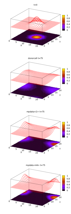
Figure 2: Plot generated by the program given in listing C.24. The top panel shows initial signal shape (at time t=0). The subsequent panels show snapshots of the advected field after 75 timesteps from three different simulations: donorcell (or 1 MPDATA iteration), MPDATA with two iterations and MPDATA with 44 iterations. The colour scale and the wire-frame surface correspond to signal amplitude. See section 2.12 for discussion.

3 Performance evaluation

The three introduced implementations of MPDATA were tested with the following set-ups employing free and open-source tools:

C++:

• GCC g++ 4.8.0 and Blitz++ 0.10

• LLVM Clang 3.2 and Blitz 0.10

Python:

• CPython 2.7.3 and NumPy 1.7

• PyPy 1.9.0 with built-in NumPy implementation

Fortran:

• GCC gfortran 4.8.0¹¹

The performance tests were run on a Debian and an Ubuntu GNU/Linux systems with the above-listed software obtained via binary packages from the distributions’ package repositories (most recent package versions at the time of writing). The tests were performed on two 64-bit machines equipped with an AMD Phenom^™ II X6 1055T (800 MHz) and an Intel^® Core^™ i5-2467M (1.6 GHz) processors.

For both C++ and Fortran the GCC compilers were invoked with the -Ofast and the -march=native options. The Clang compiler was invoked with the -O3, the -mllvm -vectorize, the -ffast-math and the -march=native options. The CPython interpreter was invoked with the -OO option.

In addition to the standard Python implementation CPython, the Python code was tested with PyPy. PyPy is an alternative implementation of Python featuring a just-in-time compiler. PyPy includes an experimental partial reimplementation of NumPy that compiles NumPy expressions into native assembler. Thanks to employment of lazy evaluation of array expressions (cf. Sect. 2.1) PyPy allows to eliminate the use of temporary matrices for storing intermediate results, and to perform multiple operations on the arrays within a single array index traversal . Consequently, PyPy allows to overcome the same performance-limiting factors as those addressed by Blitz++, although the underlying mechanisms are different. In contrast to other solutions for improving performance of NumPy-based codes such as Cython, numexpr or Numba, PyPy does not require any modifications to the code. Thus, PyPy may serve as a drop-in replacement for CPython ready to be used with previously-developed codes.

The same set of tests was run with all four set-ups. Each test set consisted of 16 program runs. The test programs are analogous to the example code presented in section 2.12. The tests were run with different grid sizes ranging from 64$\times$64 to 2048$\times$2048. The Gaussian impulse was advected for $nt=2^{24}/(nx\cdot ny)$ timesteps ($2^{24}$ chosen arbitrarily), in order to assure comparable timing accuracy for all grid sizes. Three MPDATA iterations were used (i.e. two corrective steps). The initial condition was loaded from a text file, and the final values were compared at the end of the test with values loaded from another text file assuring the same results were obtained with all four set-ups. The tests were run multiple times; program start-up, data loading, and output verification times were subtracted from the reported values (see caption of Figure 4 for details).

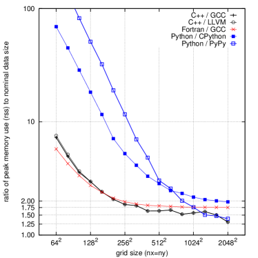
Figure 3: Memory consumption statistics for the test runs described in Section 3 plotted as a function of grid size. Peak resident set size (rss) values reported by the GNU time utility are normalised by the size of data that needs to be allocated in the program to store all declared grid-sized arrays. Asymptotic values reached at the largest grid sizes are indicative of temporary storage requirements.

Figure 3 presents a plot of the peak memory use (identical for both considered CPUs) as a function of grid size. The plotted values are normalised by the nominal size of all data arrays used in the program (i.e. two (nx+2)$\times$(ny+2) arrays representing the two time levels of $\psi$, a (nx+1)$\times$(ny+2) array representing the $C^{[x]}$ component of the Courant number field, a (nx+2)$\times$(ny+1) array representing the $C^{[y]}$ component, and two pairs of arrays of the size of $C^{[x]}$ and $C^{[y]}$ for storing the antidiffusive velocities, all composed of 8-byte double-precision floating point numbers). Plotted statistics reveal a notable memory footprint of the Python interpreter itself for both CPython and PyPy, losing its significance for domains larger than 1024$\times$1024. The roughly asymptotic values reached in all four set-ups for grid sizes larger that 1024$\times$1024 are indicative of the amount of temporary memory used for array manipulation. PyPy- and Blitz++-based set-ups consume notably less memory than Fortran and CPython. This confirms the effectiveness of the just-in-time compilation (PyPy) and the expression-templates (Blitz++) techniques for elimination of temporary storage during array operations.

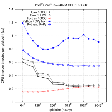
Figure 4: Execution time statistics for the test runs described in Section 3 plotted as a function of grid size. Values of the total user mode CPU time reported by the GNU time utility are normalised by the grid size ($nx\cdot ny$) and the number of timesteps $nt=2^{24}/(nx\cdot ny)$. Before normalisation the time reported for an $nt=0$ run for a corresponding domain size is subtracted from the values. Both the $nt=0$ and $nt=2^{24}/()nx\cdot ny$ runs are repeated three times and only the shortest time is taken into account. Results obtained with an Intel^® Core^™ i5 1.6 GHz processor.

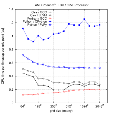
Figure 5: Same as Fig. 4 for an AMD Phenom^™ II 800 MHz processor.

The CPU time statistics presented in Figures 4 and 5 reveal minor differences between results obtained with the two different processors. Presented results lead to the following observations (where by referring to language names, only the results obtained with the herein considered program codes, and software/hardware configurations are meant):

• Fortran gives shortest execution times for any domain size;

• C++ execution times are less than twice those of Fortran for grids larger than 256$\times$256;

• CPython requires from around 4 to almost 10 times more CPU time than Fortran depending on the grid size;

• PyPy execution times are in most cases closer to C++ than to CPython.

The support for OOP features in gfortran, the NumPy support in PyPy, and the relevant optimisation mechanisms in GCC are still in active development and hence the performance with some of the set-ups may likely change with newer versions of these packages.

It is worth mentioning, that even though the three implementations are equally structured, the three considered languages have some inherent differences influencing the execution times. Notably, while Fortran and Blitz++ offer runtime array-bounds and array-shape checks as options not intended for use in production binaries, NumPy performs them always. Additionally, the C++ and Fortran set-ups may, in principle, benefit from GCC’s auto-vectorisation features which do not have yet counterparts in CPython or PyPy. Finally, Fortran uses different ordering for storing array elements in memory, but since all tests were carried out using square grids, this should not have had any impact on the performance.

The authors do expect some performance gain could be obtained by introducing into the codes some ”manual” optimisations – code rearrangements aimed solely at the purpose of increasing performance. These were avoided intentionally as they degrade code readability, should in principle be handled by the compilers, and are generally advised to be avoided [e.g. 22, section 3.12].

4 Discussion on the tradeoffs of language choice

One of the aims of this paper is to show the applicability of OOP features of the three programming languages (or language-library pairs) for scientific computing. The main focus is to represent what can be referred to as blackboard abstractions [21] within the code. Presented benchmark tests, although quite simplistic, together with the experience gained from the development of codes in three different languages provide a basis for discussion on the tradeoffs of programming language choice. The discussion concerns in principle the development of finite-difference solvers for partial differential equations, but is likely applicable to the scientific software in general. A partly objective and partly subjective summary of pros and cons of C++, Python and Fortran is presented in the four following subsections.

4.1 OOP for blackboard abstractions

It was shown in section 2 that C++11/Blitz++, Python/NumPy and Fortran 2008 provide comparable functionalities in terms of matching the blackboard abstractions within the program code. Taking into account solely the part of code representing particular formulæ  (e.g. listings C.21, P.17, F.20 and equation 4) all three languages allow to match (or surpass) LaTeX in its brevity of formula translation syntax. All three languages were shown to be capable of providing mechanisms to compactly represent such abstractions as:

• loop-free array arithmetics;

• definitions of functions returning array-valued expressions;

• permutations of array indices allowing dimension-independent definitions of functions (see e.g. listings C.12 and C.13, P.10 and P.11, F.11 and F.12);

• fractional indexing of arrays corresponding to employment of a staggered grid.

Three issues specific to Fortran that resulted in employment of a more repetitive or cumbersome syntax than in C++ or Python were observed:

• Fortran does not feature a mechanism allowing to reuse a single piece of code (algorithm) with different data types (compare e.g. listings C.6, P.5 and F.4) such as templates in C++ and the so-called duck typing in Python;

• Fortran does not allow function calls to appear on the left hand side of assignment (see e.g. how the ptr pointers were used as a workaround in the cyclic_fill_halos method in listing F.8);

• Fortran lacks support for arrays of arrays (cf. Sect. 2.2).

Interestingly, the limitation in extendability via inheritance was found to exist partially in NumPy as well (see footnote 7). The lack of a counterpart in Fortran to the C++ template mechanism was identified in [23] as one of the key deficiencies of Fortran when compared with C++ in context of applicability to object-oriented scientific programming.

4.2 Performance

The timing and memory usage statistics presented in figures 3-5 reveal that no single language/library/compiler set-up corresponded to both shortest execution time and smallest memory footprint.

One may consider performance measures addressing not only the program efficiency but also the factors influencing the development and maintenance time/cost [of particular importance in scientific computing, 24]. Taking into account such measures as code length or coding time, the Python environment gains significantly. Presented Python code is shorter than the C++ and Fortran counterparts, and is simpler in terms of syntax and usage (see discussion below).

Employment of the PyPy drop-in replacement for the standard Python implementation brings Python’s performance significantly closer to those of C++ and Fortran, in some cases making it the least memory consuming set-up. Python has already been the language of choice for scientific software projects having code clarity or ease of use as the first requirement [see e.g. 25]. PyPy’s capability to improve performance of unmodified Python code may make Python a favourable choice even if high performance is important, especially if a combined measure of performance and development cost is to be considered.

4.3 Ease of use and abuse

Using the number of lines of code or the number of distinct language keywords needed to implement the MPDATA-based solver presented in section 2 as measures of syntax brevity, Python clearly surpasses its rivals. Python was developed with emphasis on code readability and object-orientation. Arguably, taking it to the extreme - Python uses line indentation to define blocks of code and treats even single integers as objects. As a consequence Python is easy to learn and easy to teach. It is also much harder to abuse Python than C++ or Fortran (for instance with goto statements, employment of the preprocessor, or the implicit typing in Fortran).

Python implementations do not expose to the user the compilation or linking processes. As a result, Python-written software is easier to deploy and share, especially if multiple architectures and operating systems are targeted. However, there exist tools such as CMake that allow to efficiently automate building, testing and packaging of C++ and Fortran programs.

Python is definitely easiest to debug among the three languages. Great debugging tools for C++ do exist, however the debugging and development is often hindered by indecipherable compiler messages flooded with lengthy type names stemming from employment of templates. Support for the OOP features of Fortran among free and open source compilers, debuggers and other programming aids remains immature.

With both Fortran and Python, the memory footprint caused by employment of temporary objects in array arithmetics is dependant on compiler choice or the level of optimisations. In contrast, Blitz++ ensures temporary-array-free computations by design [26] avoiding unintentional performance loss.

4.4 Added values

The size of the programmers’ community of a given language influences the availability of trained personnel, reusable software components and information resources. It also affects the maturity and quality of compilers and tools. Fortran is a domain-specific language while Python and C++ are general-purpose languages with disproportionately larger users’ communities. The OOP features of Fortran have not gained wide popularity among users [27]. Fortran is no longer routinely taught at the universities [28], in contrast to C++ and Python. An example of decreasing popularity of Fortran in academia is the discontinuation of Fortran printed editions of the ”Numerical Recipes” series of Press et al.

Blitz++ is one of several packages that offer high-performance object-oriented array manipulation functionality with C++ (and is not necessarily optimal for every purpose [29]). In contrast, the NumPy package became a de facto standard solution for Python. Consequently, numerous Python libraries adopted NumPy but there are apparently very few C++ libraries offering Blitz++ support out of the box (the gnuplot-iostream used in listing C.24 being a much-appreciated counterexample). However, Blitz++ allows to interface with virtually any library (including Fortran libraries), by resorting to referencing the underlying memory with raw pointers.

The availability and quality of libraries that offer object-oriented interfaces differs among the three considered languages. The built-in standard libraries of Python and C++ are richer than those of Fortran and offer versatile data types, collections of algorithms and facilities for interaction with host operating system. In the authors’ experience, the small popularity of OOP techniques among Fortran users is reflected in the library designs (including the Fortran’s built-in library routines). What makes correct use of external libraries more difficult with Fortran is the lack of standard exception handling mechanism, a feature long and much requested by the numerical community [30, Foreword].

Finally, the three languages differ as well with regard to availability of mechanisms for leveraging shared-memory parallelisation (e.g. with multi-core processors). GCC supports OpenMP with Fortran and C++. The CPython and PyPy implementations of Python do not offer any built-in solution for multi-threading.

5 Summary and outlook

Three implementations of a prototype solver for the advection equation were introduced. The solvers are based on MPDATA - an algorithm of particular applicability in geophysical fluid dynamics [11]. All implementations follow the same object-oriented structure but are implemented in three different languages:

• C++ with Blitz++;

• Python with NumPy;

• Fortran.

Presented programs were developed making use of such recent developments as support for C++11 and Fortran 2008 in GCC, and the NumPy support in the PyPy implementation of Python. The fact that all considered standards are open and the employed tools implementing them are free and open-source is certainly an advantage [31].

The key conclusion is that all considered language/library/compiler set-ups offer possibilities for using OOP to compactly represent the mathematical abstractions within the program code. This creates the potential to improve code readability and brevity,

• contributing to its auditability, indispensable for credible and reproducible research in computational science [32, 33, 34]; and

• helping to keep the programs maintainable and avoiding accumulation of the code debt that besets scientific software in such domains as climate modelling [36].

The performance evaluation revealed that:

• the Fortran set-up offered shortest execution times,

• it took the C++ set-up less than twice longer to compute than Fortran,

• C++ and PyPy set-ups offered significantly smaller memory consumption than Fortran and CPython for larger domains,

• the PyPy set-up was roughly twice slower than C++ and up to twice faster than CPython.

The three equally-structured implementations required ca. 200, 300, and 500 lines of code in Python, C++ and Fortran, respectively.

In addition to the source code presented within the text, a set of tests and build-/test-automation scripts allowing to reproduce the analysis and plots presented in section 3 are all available in the CPC Program Library and at the project repository, and are released under the GNU GPL license [18]. The authors encourage to use the presented codes for teaching and benchmarking purposes.

The OOP design enhances the possibilities to reuse and extend the presented code. Development is underway of an object-oriented C++ library featuring concepts presented herein, supporting integration in one to three dimensions, handling systems of equations with source terms, providing miscellaneous options of MPDATA and several parallel processing approaches.

Appendix P Python code for sections 2.7–2.11

Periodic Boundaries (cf. Sect. 2.7)

  listing P.8 (Python)     96 class cyclic(object): 97   # ctor 98   def __init__(self, d, i, hlo): 99     self.d = d 100     self.left_halo = slice(i.start-hlo, i.start    ) 101     self.rght_edge = slice(i.stop -hlo, i.stop     ) 102     self.rght_halo = slice(i.stop,      i.stop +hlo) 103     self.left_edge = slice(i.start,     i.start+hlo) 104  105   # method invoked by the solver 106   def fill_halos(self, psi, j): 107     psi[pi(self.d, self.left_halo, j)] = ( 108       psi[pi(self.d, self.rght_edge, j)] 109     ) 110     psi[pi(self.d, self.rght_halo, j)] = ( 111       psi[pi(self.d, self.left_edge, j)] 112     ) 113      

Donor-cell formulæ (cf. Sect. 2.8)

  listing P.9 (Python)     114 def f(psi_l, psi_r, C): 115   return ( 116     (C + abs(C)) * psi_l + 117     (C - abs(C)) * psi_r 118   ) / 2     

  listing P.10 (Python)     119 def donorcell(d, psi, C, i, j): 120   return ( 121     f( 122       psi[pi(d, i,     j)], 123       psi[pi(d, i+one, j)], 124         C[pi(d, i+hlf, j)] 125     ) - 126     f( 127       psi[pi(d, i-one, j)], 128       psi[pi(d, i,     j)], 129         C[pi(d, i-hlf, j)] 130     ) 131   )     

  listing P.11 (Python)     132 def donorcell_op(psi, n, C, i, j): 133   psi[n+1][i,j] = (psi[n][i,j] 134     - donorcell(0, psi[n], C[0], i, j) 135     - donorcell(1, psi[n], C[1], j, i) 136   )     

Donor-cell solver (cf. Sect. 2.9)

  listing P.12 (Python)     137 class solver_donorcell(solver): 138   def __init__(self, bcx, bcy, nx, ny): 139     solver.__init__(self, bcx, bcy, nx, ny, 1) 140  141   def advop(self): 142     donorcell_op( 143       self.psi, self.n, 144       self.C, self.i, self.j 145     )     

MPDATA formulæ (cf. Sect. 2.10)

  listing P.13 (Python)     146 def mpdata_frac(nom, den): 147   return numpy.where(den > 0, nom/den, 0)     

  listing P.14 (Python)     148 def mpdata_A(d, psi, i, j): 149   return mpdata_frac( 150     psi[pi(d, i+one, j)] - psi[pi(d, i, j)], 151     psi[pi(d, i+one, j)] + psi[pi(d, i, j)] 152   )     

  listing P.15 (Python)     153 def mpdata_B(d, psi, i, j): 154   return mpdata_frac( 155     psi[pi(d, i+one, j+one)] + psi[pi(d, i, j+one)] - 156     psi[pi(d, i+one, j-one)] - psi[pi(d, i, j-one)], 157     psi[pi(d, i+one, j+one)] + psi[pi(d, i, j+one)] + 158     psi[pi(d, i+one, j-one)] + psi[pi(d, i, j-one)] 159   ) / 2     

  listing P.16 (Python)     160 def mpdata_C_bar(d, C, i, j): 161   return ( 162     C[pi(d, i+one, j+hlf)] + C[pi(d, i,  j+hlf)] + 163     C[pi(d, i+one, j-hlf)] + C[pi(d, i,  j-hlf)] 164   ) / 4     

  listing P.17 (Python)     165 def mpdata_C_adf(d, psi, i, j, C): 166   return ( 167     abs(C[d][pi(d, i+hlf, j)]) 168     * (1 - abs(C[d][pi(d, i+hlf, j)])) 169     * mpdata_A(d, psi, i, j) 170     - C[d][pi(d, i+hlf, j)] 171     * mpdata_C_bar(d, C[d-1], i, j) 172     * mpdata_B(d, psi, i, j) 173   )     

An MPDATA solver (cf. Sect. 2.11)

  listing P.18 (Python)     174 class solver_mpdata(solver): 175   def __init__(self, n_iters, bcx, bcy, nx, ny): 176     solver.__init__(self, bcx, bcy, nx, ny, 1) 177     self.im = slice(self.i.start-1, self.i.stop) 178     self.jm = slice(self.j.start-1, self.j.stop) 179  180     self.n_iters = n_iters 181  182     self.tmp = [( 183       numpy.empty(self.C[0].shape, real_t), 184       numpy.empty(self.C[1].shape, real_t) 185     )] 186     if n_iters > 2: 187       self.tmp.append(( 188         numpy.empty(self.C[0].shape, real_t), 189         numpy.empty(self.C[1].shape, real_t) 190       )) 191  192   def advop(self): 193     for step in range(self.n_iters): 194       if step == 0: 195         donorcell_op( 196           self.psi, self.n, self.C, self.i, self.j 197         ) 198       else: 199         self.cycle() 200         self.bcx.fill_halos( 201           self.psi[self.n], ext(self.j, self.hlo) 202         ) 203         self.bcy.fill_halos( 204           self.psi[self.n], ext(self.i, self.hlo) 205         ) 206         if step == 1: 207           C_unco, C_corr = self.C, self.tmp[0] 208         elif step % 2: 209           C_unco, C_corr = self.tmp[1], self.tmp[0] 210         else: 211           C_unco, C_corr = self.tmp[0], self.tmp[1] 212  213         C_corr[0][self.im+hlf, self.j] = mpdata_C_adf( 214           0, self.psi[self.n], self.im, self.j, C_unco 215         ) 216         self.bcy.fill_halos(C_corr[0], ext(self.i, hlf)) 217  218         C_corr[1][self.i, self.jm+hlf] = mpdata_C_adf( 219           1, self.psi[self.n], self.jm, self.i, C_unco 220         ) 221         self.bcx.fill_halos(C_corr[1], ext(self.j, hlf)) 222  223         donorcell_op( 224           self.psi, self.n, C_corr, self.i, self.j 225         )     

Usage example (cf. Sect. 2.12)

  listing P.19 (Python)     226   slv = solver_mpdata(it, cyclic, cyclic, nx, ny) 227   slv.state()[:] = read_file(fname, nx, ny) 228   slv.courant(0)[:] = Cx 229   slv.courant(1)[:] = Cy 230   slv.solve(nt)     

Appendix F Fortran code for sections 2.7–2.11

Periodic boundaries (cf. Sect. 2.7)

  listing F.8 (Fortran)     268 module cyclic_m 269   use bcd_m 270   use pi_m 271   implicit none 272    273   type, extends(bcd_t) :: cyclic_t 274     integer :: d 275     integer :: left_halo(2), rght_halo(2) 276     integer :: left_edge(2), rght_edge(2) 277     contains 278     procedure :: init => cyclic_init 279     procedure :: fill_halos => cyclic_fill_halos 280   end type 281  282   contains 283  284   subroutine cyclic_init(this, d, n, hlo) 285     class(cyclic_t) :: this 286     integer :: d, n, hlo 287  288     this%d = d 289     this%left_halo = (/ -hlo, -1 /) 290     this%rght_halo = (/ n, n-1+hlo /) 291     this%left_edge = (/ 0, hlo-1 /) 292     this%rght_edge = (/ n-hlo, n-1 /) 293   end subroutine 294  295   subroutine cyclic_fill_halos(this, a, j) 296     class(cyclic_t) :: this 297     real(real_t), pointer :: ptr(:,:) 298     real(real_t), allocatable :: a(:,:) 299     integer :: j(2) 300     ptr => pi(this%d, a, this%left_halo, j) 301     ptr =  pi(this%d, a, this%rght_edge, j) 302     ptr => pi(this%d, a, this%rght_halo, j) 303     ptr =  pi(this%d, a, this%left_edge, j) 304   end subroutine 305 end module     

Donor-cell formulæ (cf. Sect. 2.8)

  listing F.9 (Fortran)     306 module donorcell_m 307   use real_m 308   use arakawa_c_m 309   use pi_m 310   use arrvec_m 311   implicit none 312   contains     

  listing F.10 (Fortran)     313   elemental function F(psi_l, psi_r, C) result (return) 314     real(real_t) :: return 315     real(real_t), intent(in) :: psi_l, psi_r, C 316     return = (                                         & 317       (C + abs(C)) * psi_l +                           & 318       (C - abs(C)) * psi_r                             & 319     ) / 2 320   end function     

  listing F.11 (Fortran)     321   function donorcell(d, psi, C, i, j) result (return) 322     integer :: d 323     integer, intent(in) :: i(2), j(2) 324     real(real_t) :: return(span(d, i, j), span(d, j, i)) 325     real(real_t), allocatable, intent(in) :: psi(:,:), C(:,:) 326     return = (                                         & 327       F(                                               & 328         pi(d, psi, i,   j),                            & 329         pi(d, psi, i+1, j),                            & 330         pi(d,   C, i+h, j)                             & 331       ) -                                              & 332       F(                                               & 333         pi(d, psi, i-1, j),                            & 334         pi(d, psi, i,   j),                            & 335         pi(d, C,   i-h, j)                             & 336       )                                                & 337     ) 338   end function     

  listing F.12 (Fortran)     339   subroutine donorcell_op(psi, n, C, i, j) 340     class(arrvec_t), allocatable :: psi 341     class(arrvec_t), pointer :: C 342     integer, intent(in) :: n 343     integer, intent(in) :: i(2), j(2) 344  345     real(real_t), pointer :: ptr(:,:) 346     ptr => pi(0, psi%at(n+1)%p%a, i, j) 347     ptr = pi(0, psi%at(n)%p%a, i, j)                   & 348       - donorcell(0, psi%at(n)%p%a, C%at(0)%p%a, i, j) & 349       - donorcell(1, psi%at(n)%p%a, C%at(1)%p%a, j, i) 350   end subroutine     

  listing F.13 (Fortran)     351 end module     

Donor-cell solver (cf. Sect. 2.9)

  listing F.14 (Fortran)     352 module solver_donorcell_m 353   use donorcell_m 354   use solver_m 355   implicit none 356    357   type, extends(solver_t) :: donorcell_t 358     contains 359     procedure :: ctor => donorcell_ctor 360     procedure :: advop => donorcell_advop 361   end type 362  363   contains 364    365   subroutine donorcell_ctor(this, bcx, bcy, nx, ny) 366     class(donorcell_t) :: this 367     class(bcd_t), intent(in), target :: bcx, bcy 368     integer, intent(in) :: nx, ny 369     call solver_ctor(this, bcx,bcy, nx,ny, 1) 370   end subroutine 371  372   subroutine donorcell_advop(this) 373     class(donorcell_t), target :: this 374     class(arrvec_t), pointer :: C 375     C => this%C 376     call donorcell_op(                                 & 377       this%psi, this%n, C, this%i, this%j              & 378     ) 379   end subroutine 380 end module     

MPDATA formulæ (cf. Sect. 2.10)

  listing F.15 (Fortran)     381 module mpdata_m 382   use arrvec_m 383   use arakawa_c_m 384   use pi_m 385   implicit none 386   contains     

  listing F.16 (Fortran)     387   function mpdata_frac(nom, den) result (return) 388     real(real_t), intent(in) :: nom(:,:), den(:,:) 389     real(real_t) :: return(size(nom, 1), size(nom, 2)) 390     where (den > 0) 391       return = nom / den 392     elsewhere 393       return = 0 394     end where 395   end function     

  listing F.17 (Fortran)     396   function mpdata_A(d, psi, i, j) result (return) 397     integer :: d 398     real(real_t), allocatable, intent(in) :: psi(:,:) 399     integer, intent(in) :: i(2), j(2) 400     real(real_t) :: return(span(d, i, j), span(d, j, i)) 401     return = mpdata_frac(                              & 402       pi(d, psi, i+1, j) - pi(d, psi, i, j),           & 403       pi(d, psi, i+1, j) + pi(d, psi, i, j)            & 404     ) 405   end function     

  listing F.18 (Fortran)     406   function mpdata_B(d, psi, i, j) result (return) 407     integer :: d 408     real(real_t), allocatable, intent(in) :: psi(:,:) 409     integer, intent(in) :: i(2), j(2) 410     real(real_t) :: return(span(d, i, j), span(d, j, i)) 411     return = mpdata_frac(                              & 412       pi(d, psi, i+1, j+1) + pi(d, psi, i,   j+1)      & 413     - pi(d, psi, i+1, j-1) - pi(d, psi, i,   j-1),     & 414       pi(d, psi, i+1, j+1) + pi(d, psi, i,   j+1)      & 415     + pi(d, psi, i+1, j-1) + pi(d, psi, i,   j-1)      & 416     ) / 2 417   end function     

  listing F.19 (Fortran)     418   function mpdata_C_bar(d, C, i, j) result (return) 419     integer :: d 420     real(real_t), allocatable, intent(in) :: C(:,:) 421     integer, intent(in) :: i(2), j(2) 422     real(real_t) :: return(span(d, i, j), span(d, j, i)) 423  424     return = (                                         & 425       pi(d, C, i+1, j+h) + pi(d, C, i,   j+h) +        & 426       pi(d, C, i+1, j-h) + pi(d, C, i,   j-h)          & 427     ) / 4 428   end function     

  listing F.20 (Fortran)     429   function mpdata_C_adf(d, psi, i, j, C) result (return) 430     integer :: d 431     integer, intent(in) :: i(2), j(2) 432     real(real_t) :: return(span(d, i, j), span(d, j, i)) 433     real(real_t), allocatable, intent(in) :: psi(:,:) 434     class(arrvec_t), pointer :: C 435     return =                                           & 436       abs(pi(d, C%at(d)%p%a, i+h, j))                  & 437       * (1 - abs(pi(d, C%at(d)%p%a, i+h, j)))          & 438       * mpdata_A(d, psi, i, j)                         & 439       - pi(d, C%at(d)%p%a, i+h, j)                     & 440       * mpdata_C_bar(d, C%at(d-1)%p%a, i, j)           & 441       * mpdata_B(d, psi, i, j) 442   end function     

  listing F.21 (Fortran)     443 end module     

An MPDATA solver (cf. Sect. 2.11)

  listing F.22 (Fortran)     444 module solver_mpdata_m 445   use solver_m 446   use mpdata_m 447   use donorcell_m 448   use halo_m 449   implicit none 450    451   type, extends(solver_t) :: mpdata_t 452     integer :: n_iters, n_tmp 453     integer :: im(2), jm(2) 454     class(arrvec_t), pointer :: tmp(:) 455     contains 456     procedure :: ctor => mpdata_ctor 457     procedure :: advop => mpdata_advop 458   end type 459  460   contains 461  462   subroutine mpdata_ctor(this, n_iters, bcx, bcy, nx, ny) 463     class(mpdata_t) :: this 464     class(bcd_t), target :: bcx, bcy 465     integer, intent(in) :: n_iters, nx, ny 466     integer :: c 467  468     call solver_ctor(this, bcx, bcy, nx, ny, 1) 469  470     this%n_iters = n_iters 471     this%n_tmp = min(n_iters - 1, 2) 472     if (n_iters > 0) allocate(this%tmp(0:this%n_tmp)) 473  474     associate (i => this%i, j => this%j, hlo => this%hlo) 475       do c=0, this%n_tmp - 1 476         call this%tmp(c)%ctor(2) 477         call this%tmp(c)%init(0, ext(i, h), ext(j, hlo)) 478         call this%tmp(c)%init(1, ext(i, hlo), ext(j, h)) 479       end do 480  481       this%im = (/ i(1) - 1, i(2) /) 482       this%jm = (/ j(1) - 1, j(2) /) 483     end associate 484   end subroutine 485  486   subroutine mpdata_advop(this) 487     class(mpdata_t), target :: this 488     integer :: step 489  490     associate (i => this%i, j => this%j, im => this%im,& 491       jm => this%jm, psi => this%psi, n => this%n,     & 492       hlo => this%hlo, bcx => this%bcx, bcy => this%bcy& 493     ) 494       do step=0, this%n_iters-1 495         if (step == 0) then 496           block 497             class(arrvec_t), pointer :: C 498             C => this%C 499             call donorcell_op(psi, n, C, i, j) 500           end block 501         else 502           call this%cycle() 503           call bcx%fill_halos(                         & 504             psi%at( n )%p%a, ext(j, hlo)               & 505           ) 506           call bcy%fill_halos(                         & 507             psi%at( n )%p%a, ext(i, hlo)               & 508           ) 509  510           block 511             class(arrvec_t), pointer :: C_corr, C_unco 512             real(real_t), pointer :: ptr(:,:) 513  514             ! chosing input/output for antidiff. C 515             if (step == 1) then 516               C_unco => this%C 517               C_corr => this%tmp(0) 518             else if (mod(step, 2) == 1) then 519               C_unco => this%tmp(1) ! odd step 520               C_corr => this%tmp(0) ! even step 521             else 522               C_unco => this%tmp(0) ! odd step 523               C_corr => this%tmp(1) ! even step 524             end if 525  526             ! calculating the antidiffusive velo 527             ptr => pi(0, C_corr%at( 0 )%p%a, im+h, j) 528             ptr = mpdata_C_adf(                        & 529               0, psi%at( n )%p%a, im, j, C_unco        & 530             ) 531             call bcy%fill_halos(                       & 532               C_corr%at(0)%p%a, ext(i, h)              & 533             ) 534  535             ptr => pi(0, C_corr%at( 1 )%p%a, i, jm+h) 536             ptr = mpdata_C_adf(                        & 537               1, psi%at( n )%p%a, jm, i, C_unco        & 538             ) 539             call bcx%fill_halos(                       & 540               C_corr%at(1)%p%a, ext(j, h)              & 541             ) 542  543             ! donor-cell step 544             call donorcell_op(psi, n, C_corr, i, j) 545           end block 546         end if 547       end do 548     end associate 549   end subroutine 550 end module     

Usage example (cf. Sect. 2.12)

  listing F.23 (Fortran)     551     type(mpdata_t) :: slv 552     type(cyclic_t), target :: bcx, bcy 553     integer :: nx, ny, nt, it 554     real(real_t) :: Cx, Cy 555     real(real_t), pointer :: ptr(:,:)     

  listing F.24 (Fortran)     556     call slv%ctor(it, bcx, bcy, nx, ny) 557  558     ptr => slv%state() 559     call read_file(fname, ptr) 560  561     ptr => slv%courant(0) 562     ptr = Cx 563  564     ptr => slv%courant(1) 565     ptr = Cy 566  567     call slv%solve(nt)

References

- Press et al. [2007] W. Press, S. Teukolsky, W. Vetterling, B. Flannery, Numerical Recipes. The Art of Scientific Computing, Cambridge University Press, third edition, 2007.
- Griffies et al. [2000] S. Griffies, C. Boning, F. Bryan, E. Chassignet, R. Gerdes, H. Hasumi, A. Hirst, A.-M. Treguier, D. Webb, Developments in ocean climate modelling, Ocean Model. 2 (2000) 123–192.
- Sundberg [2009] M. Sundberg, The everyday world of simulation modeling: The development of parameterizations in meteorology, Sci. Technol. Hum. Val. 34 (2009) 162–181.
- Legutke [2012] S. Legutke, Building Earth system models, in: R. Ford, G. Riley, R. Budich, R. Redler (Eds.), Earth System Modelling - Volume 5: Tools for Configuring, Building and Running Models, 2012, pp. 45–54.
- Norton et al. [2007] C. Norton, V. Decyk, B. Szymanski, H. Gardner, The transition and adoption to modern programming concepts for scientific computing in Fortran, Sci. Prog. 15 (2007) 27–44.
- Knuth [1974] D. Knuth, Structured programming with go to statements, Comput. Surv. 6 (1974) 261–301.
- Smolarkiewicz [1984] P. Smolarkiewicz, A fully multidimensional positive definite advection transport algorithm with small implicit diffusion, J. Comp. Phys. 54 (1984) 325–362.
- Ziemiański et al. [2011] M. Ziemiański, M. Kurowski, Z. Piotrowski, B. Rosa, O. Fuhrer, Toward very high horizontal resolution NWP over the Alps: Influence of increasing model resolution on the flow pattern, Acta Geophys. 59 (2011) 1205–1235.
- Abiodun et al. [2011] B. Abiodun, W. Gutowski, A. Abatan, J. Prusa, CAM-EULAG: A non-hydrostatic atmospheric climate model with grid stretching, Acta Geophys. 59 (2011) 1158–1167.
- Ezer et al. [2002] T. Ezer, H. Arango, A. Shchepetkin, Developments in terrain-following ocean models: intercomparisons of numerical aspects, Ocean Model. 4 (2002) 249–267.
- Smolarkiewicz [2006] P. Smolarkiewicz, Multidimensional positive definite advection transport algorithm: an overview, Int. J . Numer. Meth. Fluids 50 (2006) 1123–1144.
- ISO/IEC [2011] ISO/IEC, 14882:2011 (C++11 language standard), 2011.
- Rossum [2011] G. Rossum, The Python Language Reference Manual, Network Theory, 2011. Version 3.2, ISBN 978-1-906966-14-0.
- ISO/IEC [2010] ISO/IEC, 1539-1:2010 (FORTRAN 2008 language standard), 2010.
- Stroustrup [2000] B. Stroustrup, The C++ Programming Language, Addison Wesley, third edition, 2000.
- Pilgrim [2004] M. Pilgrim, Dive Into Python, Apress, 2004.
- Markus [2012] A. Markus, Modern Fortran in Practice, Cambridge University Press, 2012.
- Stallman et al. [2007] R. Stallman, et al., GNU General Public License, Free Software Foundation, 2007. Version 3.
- Bolz et al. [2011] C. Bolz, A. Cuni, M. Fijałkowski, M. Leuschel, S. Pedroni, A. Rigo, Runtime feedback in a meta-tracing JIT for efficient dynamic languages, in: ICOOOLPS ’11 Proceedings of the 6th Workshop on Implementation, Compilation, Optimization of Object-Oriented Languages, Programs and Systems.
- Arakawa and Lamb [1977] A. Arakawa, V. R. Lamb, Computational design of the basic dynamical process of the UCLA general circulation model, in: Methods in Computational Physics, volume 17, Academic Press, New York, 1977, pp. 173–265.
- Rouson et al. [2012] D. Rouson, J. Xia, X. Xu, Scientific Software Design. The Object-Oriented Way, Cambridge University Press, 2012.
- Paoli [2000] S. Paoli, C++ Coding Standard Specification, Technical Report, CERN European Laboratory for Particle Physics, 2000.
- Cary et al. [2011] J. Cary, S. Shasharina, J. Cummings, J. Reynders, P. Hinker, Comparison of C++ and Fortran 90 for object-oriented scientific programming, Comp. Phys. Comm. (2011).
- Wilson [2006] G. Wilson, Where’s the real bottleneck in scientific computing?, Am. Sci. 94 (2006) 5–6.
- Barnes and Jones [2011] N. Barnes, D. Jones, Clear climate code: Rewriting legacy science software for clarity, IEEE Software (2011) 36–42.
- Veldhuizen and Jernigan [1997] T. Veldhuizen, M. Jernigan, Will C++ be faster than fortran?, in: Y. Ishikawa, R. Oldehoeft, J. Reynders, M. Tholburn (Eds.), Scientific Computing in Object-Oriented Parallel Environments, volume 1343 of Lecture Notes in Computer Science, Springer Berlin / Heidelberg, 1997, pp. 49–56.
- Worth [2008] D. Worth, State of the Art in Object Oriented Programming with Fortran, Technical Report, Science and Technology Facilities Council, 2008. RAL-TR-2008-002.
- Kendall et al. [2008] R. Kendall, D. Fisher, D. Henderson, J. Carver, A. Mark, D. Post, C. J. Rhoades, S. Squires, Development of a weather forecasting code: A case study, IEEE Software (2008).
- Iglberger et al. [2012] K. Iglberger, G. Hager, J. Treibig, U. Rüde, Expression templates revisited: a performance analysis of current methodologies, SIAM J. Sci. Comput. 34 (2012) C42–C69.
- Press et al. [2007] W. Press, S. Teukolsky, W. Vetterling, B. Flannery, Numerical Recipes in Fortran 90. The Art of Parallel Scientific Computing, Cambridge University Press, second edition, 2007.
- Añel [2011] J. Añel, The importance of reviewing the code, Comm. ACM 54 (2011) 40–41.
- Post and Votta [2005] D. Post, L. Votta, Computational science demands a new paradigm, Phys. Today 58 (2005).
- Merali [2010] Z. Merali, Why scientific programming does not compute, Nature 467 (2010) 775–777.
- Stodden et al. [2012] V. Stodden, I. Mitchell, R. LeVeque, Reproducible research for scientific computing: Tools and strategies for changing the culture, Comput. Sci. Eng. 14 (2012) 13–17.
- Buschmann [2011] F. Buschmann, To pay or not to pay technical debt, IEEE Software 28 (2011) 29–31.
- Freeman et al. [2010] S. Freeman, T. Clune, R. I. Burns, Latent risks and dangers in the state of climate model software development, in: Proceedings of the FSE/SDP workshop on Future of software engineering research, ACM, 2010, pp. 111–114.