Solar differential rotation: hints to reproduce a near-surface shear layer in global simulations

Abstract

Convective turbulent motions in the solar interior, as well as the mean flows resulting from them, determine the evolution of the solar magnetic field. With the aim to get a better understanding of these flows we study anelastic rotating convection in a spherical shell whose stratification resembles that of the solar interior. This study is done through numerical simulations performed with the EULAG code. Due to the numerical formulation, these simulations are known as implicit large eddy simulations (ILES), since they intrinsically capture the contribution of, non-resolved, small scales at the same time maximizing the effective Reynolds number. We reproduce some previous results and find a transition between buoyancy and rotation dominated regimes which results in anti-solar or solar like rotation patterns. Even thought the rotation profiles are dominated by Taylor-Proudman columnar rotation, we are able to reproduce the tachocline and a low latitude near-surface shear layer. We find that simulations results depend on the grid resolution as a consequence of a different sub-grid scale contribution.

1 Introduction

The dynamo mechanism, presumably governing the cyclic evolution of the global magnetic field in the Sun (also in late type stars and galaxies as well as planets), depends on both, the small and large scale motions in the solar interior. Within the mean-field theoretical framework, two mechanisms are invoked to explain a dynamo cycle. These are so called $\Omega$ and $\alpha$ effects. The first one depends on the differential rotation (large scale motion), i.e., the amount of shear able to stretch the magnetic field lines. The second effect is the contribution of the helical turbulent motions to the amplification of magnetic field. It only exists in systems that lack reflectional symmetry (i.e., rotating systems). Turbulent diffusivity is another important ingredient for a dynamo, and other small-scale phenomena like turbulent pumping ([Guerrero & de Gouveia Dal Pino (2008), Guerrero & de Gouveia Dal Pino, 2008]) or the shear-current effect (e.g. [Pipin & Kosovichev (2011), Pipin & Kosovichev, 2011]) might also play a role.

From the large variety of solar dynamo solutions, the Babcock-Leighton (BL) flux-transport models are particularly popular since they result in magnetic field evolution (sunspot butterfly diagrams) that resemble the observations. The BL mechanism is a phenomenological formulation of an $\alpha$-effect that depends on the turbulent diffusion of the magnetic flux of active regions and the poleward transport of magnetic field by meridional flow. Due to this meridional flow the polar magnetic flux of a previous cycle is replaced by magnetic flux of opposite polarity. The polar field is then transported downward towards the base of the convection zone where magnetic flux tubes are thought to be formed. However, the results of BL and other mean-field models are ambiguous in the sense that different combinations of parameters equally resemble the observations. Making thus difficult to discern what are the correct ones. Recent helioseismic results indicate that there may be two circulation cells per meridional quadrant ([ZK12, see the contribution of Zhao et al. in this proceedings]), and BL models with such meridional flow profile fail to reproduce the observations ([Jouve & Brun (2007), Jouve and Brun, 2007]). Besides, the emergence of magnetic flux tubes from the base of the convection zone to the surface is still a matter of debate ([Guerrero & Käpylä (2011), Guerrero & Käpylä, 2011]).

Another attractive alternative, not sufficiently explored so far, to explain the solar magnetic cycle is a distributed dynamo, where the turbulent $\alpha$ effect operates in the entire convection zone and not only at the boundaries as in BL models. The observed migration pattern corresponds, however, to a dynamo wave traveling equatorwards in a thin layer near the surface where the shear is negative ([Brandenburg (2005), Brandenburg, 2005], [Pipin & Kosovichev (2011), Pipin & Kosovichev, 2011]). The rotation of sunspots, faster than the surface plasma rotation, is one of the arguments in favor of this alternative. This model does not depend strongly on the meridional flow and does not require magnetic field above equipartition as the buoyancy of flux tubes model does. Explaining the sunspot formation and their properties in this model is still problematic, but these phenomena are in general still an open question and deserve further study.

To advance our understanding of the solar dynamo mechanism it is important to understand first the dynamics of the flows in the convection zone. From a theoretical point of view, the most realistic approach to study the solar flows is through global numerical simulations (GNS). Although the current computing capabilities are unable to resolve the essential scales in the Sun, GNS are able to study systems that resemble some of the solar properties. The main expectation is to get closer to the reality and understand the complicated multi-scale physics. Since the first global numerical models (e.g. [Gilman (1977), Gilman, 1977]) there has been huge progress in the understanding of convection in rotating spherical shells, but till now, ab-initio 3D numerical models still have difficulties in reproducing the observed properties of the solar differential rotation (e.g. [Miesch et al. (2006), Miesch et al., 2006], [Käpylä et al. (2011), Käpylä et al. 2011]). To our knowledge just a few groups are addressing this problem. The ASH group (e.g., [Miesch et al. (2006), Miesch et al., 2006]) uses an anelastic, spectral code (as well as [BS11, Busse & Simitiev, 2010]), the Pencil-Code group (e.g., [Käpylä et al. (2011), Käpylä et al. 2011]) which uses finite differences to perform compressible simulations in a wedge geometry and the EULAG group (e.g., [GC10, Ghizaru et al., 2010]), which so far has focused on the solar dynamo rather than on the differential rotation problem.

In this paper we present the initial results of our attempt to address the differential rotation problem with the EULAG code ([Smolarkiewicz et al. (2001), Smolarkiewicz et al., 2001], [Prusa et al. (2008), Prusa et al., 2008]). EULAG is an anelastic code for geosphysical and astrophysical fluid dynamics, with unique semi-implicit numerics built on high-resolution nonoscillatory forward-in-time (NFT) advection schemes MPDATA (for multidimensional positive definite advection transport algorithm); cf. [Smolarkiewicz (2006), Smolarkiewicz, 2006] for a recent overview. The code does not require any explicit viscosity in order to remain stable, and the numerical viscosity has been identified to work similarly to the eddy viscosity used in different sub-grid scale models ([Margolin & Rider (2002), Margolin & Rider, 2002]). For this reason EULAG results are interpreted as ILES ([Smolarkiewicz & Margolin (2007), Smolarkiewicz & Margolin, 2007]).

2 Model setup

We solve the anelastic set of hydrodynamic equations following the formulation of [Lipps & Hemler (1982)] and [Lipps (1990)]:

$${\bm{\nabla}}\cdot(\rho_{s}\bm{u})=0,$$ (1)

$$\frac{D\bm{u}}{Dt}=2{\bm{\Omega}}\times{\bm{u}}+{\bf g}\frac{\Theta^{\prime}}{\Theta_{s}}-{\bm{\nabla}}\left(\frac{p^{\prime}}{\rho_{s}}\right)\;,$$ (2)

$$\frac{D\Theta^{\prime}}{Dt}=-{\bm{u}}\cdot{\bm{\nabla}}\Theta_{e}+\frac{1}{\rho_{s}}{\cal H}(\Theta^{\prime})-\alpha\Theta^{\prime}$$ (3)

where $D/Dt=\partial/\partial t+\bm{u}\cdot{\bm{\nabla}}$ is the total time derivative, ${\bm{u}}$, is the velocity, $p^{\prime}$ and $\Theta^{\prime}$ are the pressure and potential temperature fluctuations, respectively and $\cal{H}(\theta^{\prime})$ absorbs the radiative and heat diffusion terms. $\rho_{s}$ and $\Theta_{s}$ are the density and potential temperature of the reference state chosen to be isentropic. The radial profile of $\rho_{s}$ is defined considering hydrostatic equilibrium with $g\propto 1/r^{2}$ and $\Theta_{s}={\rm const}$. The potential temperature is related to the specific entropy via $s=c_{p}\ln\Theta+{\rm const}$. In Eq.  (2) ${\bm{\Omega}}$ is the rotation vector. Finally, $\Theta_{e}$ is the potential temperature of an ambient state which is assumed to be an azimuthal and long-term temporal average of a static solution of the system. The term $\alpha\Theta^{\prime}$ in eq. (3), forces the system towards the ambient state, $\Theta_{e}$, on a timescale $\tau=\alpha^{-1}=1.55{\rm e}8$ s. This timescale is much shorter than the timescale of radiative and heat diffusion, meaning that this term ultimately drives convection in the system. The fact that the Sun does not exhibit important changes in its thermal state over the time scale of our interest, make us to believe that a 1D solar structural model is a good approximation for the ambient state of the solar interior.

For the simulations presented here we approximate the ambient state by a polytropic model. Our domain spans in radius from $0.62R_{\odot}$ to $0.96R_{\odot}$ (although in the final section we extend our domain up to $r=0.985R_{\odot}$). From the bottom up to $r=0.71R_{\odot}$ the model is stable to convection with polytropic index $m=3$. The upper layer is convectively unstable with $m=1.49995$. In latitude and longitude we consider $0\leq\theta\leq\pi$ and $0\leq\phi\leq 2\pi$, respectively. In the latitudinal direction discrete differentiation extends across the poles, while flipping sign of the latitudinal and meridional components of differentiated vector fields. In the radial direction we use stress free, impermeable, boundary conditions for the velocity field, whereas for $\Theta^{\prime}$ zero normal derivative is assumed.

3 Results

We have performed spherical shell convection simulations aiming to reproduce the solar differential rotation. As mentioned in the previous section, our numerical model does not explicitly include dissipative terms. For this reason, it is not easy to determine precise values of non-dimensional quantities like the Reynolds, Rayleight or Taylor numbers ([Domaradzki et al. (2003), Domaradzki et al., 2003]). For this paper we characterize our simulations with the rotation rate and the grid resolution.

3.1 Convection vs. rotation

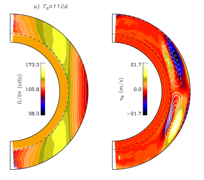
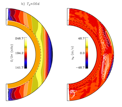
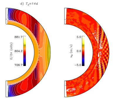
Figure 1: Differential rotation and meridional circulation profiles for the models with different rotation period, $T_{0}$, as indicated in the legend. The profiles correspond to longitude-time averages computed in the, statistically, steady stage during a 3-years time span. Continuous (dashed) lines depict clockwise (counterclockwise) contours of the stream flow. They represent the meridional circulation profile.

In the first set of simulations we consider models with different rotation period and keep constant all other parameters. We study cases with $T_{0}=112d$ ($\Omega_{0}=0.25\Omega_{\odot}$, (case L0.25), $T_{0}=56d$ ($0.5\Omega_{\odot}$, L0.5), $T_{0}=28d$ ($\Omega_{\odot}$, L1) and $T_{0}=14d$ ($2\Omega_{\odot}$, L2). These simulations are performed with a rather coarse resolution ($n_{\phi}=128$, $n_{\theta}=64$, $n_{r}=47$) previously adopted by [GC10, Ghizaru et al. (2010)]. The results are shown in Fig. 1.

As it was described in [Gilman (1977)], the resulting rotation pattern is defined by the ratio between the rotation rate and the amplitude of the convective velocities, i.e., by the competition between Coriolis vs. buoyant forces. Our results agree with previous studies of rotating convection ([Käpylä et al. (2011), Käpylä et al. 2011]). For the slow rotating cases buoyancy dominates, the correlation between the azimuthal and the vertical velocities, $R_{r\phi}=\langle u_{r}^{\prime}u_{\phi}^{\prime}\rangle$, is mainly negative so that there is an inwards transfer of angular momentum. Probably due to the meridional Reynolds stress component, $R_{r\theta}=\langle u_{r}^{\prime}u_{\theta}^{\prime}\rangle$, a single meridional circulation cell at each meridional quadrant is formed. It is counterclockwise in the northern and clockwise in the southern hemispheres. This circulation, in turn, redistributes via advection the angular momentum leading to faster rotation at higher latitudes.

With the increase of the rotation rate, Coriolis forces dominates over buoyancy. The latitudinal component of the Reynolds stress tensor, $R_{\theta\phi}=\langle u_{\theta}^{\prime}u_{\phi}^{\prime}\rangle$, results positive (negative) in the northern (southern) hemisphere and tends to concentrate at lower latitudes at the base of the convection zone ([GSK13, Guerrero et al. (2013), in preparation]). The tensor component $R_{r\phi}$, which is symmetric across the equator, changes sign for $\Omega_{0}\geq\Omega_{\odot}$, switching the rotation profile from decelerated to accelerated in the equatorial region. In these cases the meridional circulation is multicellular and does not seem to significantly affect the distribution of angular momentum. The contrast in rotation between the equator and $60^{\circ}$ latitude in case L1 is $\Delta\Omega\simeq 80$ nHz, in good agreement with the Sun where this difference is $\sim 85$ nHz.

As it has been found in previous solar simulations with EULAG (i.e. [Ghizaru et al. (2010), Ghizaru et al. 2010], [Racine et al. (2011), Racine et al. 2011]), the rotation profile exhibits a well defined tachocline. It appears due to a strongly sub-adiabatic layer ($r<0.71R_{\odot}$) obtained with a steeper profile of $\Theta_{e}$. Numerical experiments not included here, with a less steeper $\Theta_{e}$ profile between the two regions, result in the transfer of angular momentum towards the stable region. The mean flows resulting from those models dramatically differ from the ones reported here.

The profiles of differential rotation for most of the simulations show alignment of iso-rotation lines along the rotation axis (Taylor-Proudman theorem). For the case L1, a slight departure from this columnar distribution starts to appear at latitudes above $\sim 70^{\circ}$. A solar-like profile, with conical contours of iso-rotation could be achieved with the fine setting of some model parameters (Charbonneau et al. 2012, private communication).

The meridional flow, depicted in Fig. 1 with continuous lines, corresponds to a clockwise circulation, dashed lines correspond to counterclockwise circulation. It varies from a single, coherent, cell at each hemisphere for the case L0.25 to a double cell configuration for case L0.5 and a multicellular, not well defined, pattern for cases L1 and L2 ($\Omega_{0}\geq\Omega_{\odot}$).

3.2 Convergence experiments

In the next set of numerical experiments we keep the period of rotation fixed to the solar value ($\Omega_{0}=\Omega_{\odot}$) and explore the effects of the implicit LES viscosity and the convergence of the results by increasing the resolution. We denote these models as case L1 ($n_{\phi}=128$, $n_{\theta}=64$, $n_{r}=47$), M1 ($n_{\phi}=256$, $n_{\theta}=128$, $n_{r}=94$) and H1 ($n_{\phi}=512$, $n_{\theta}=256$, $n_{r}=188$).

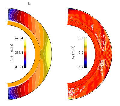
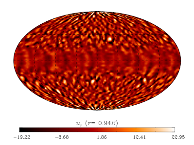
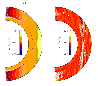
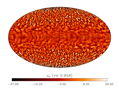
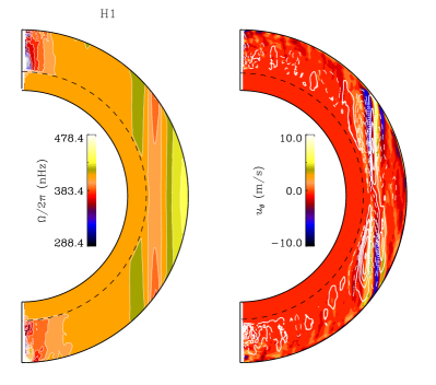
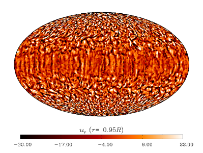
Figure 2: Left: differential rotation profiles for models with different numerical resolution. Models L1 ($n_{\phi}=128$, $n_{\theta}=64$, $n_{r}=47$), M1 ($n_{\phi}=256$, $n_{\theta}=128$, $n_{r}=94$), and H1 ($n_{\phi}=512$, $n_{\theta}=256$, $n_{r}=188$) are shown from top to bottom. Middle: meridional circulation profiles. Right: vertical velocity (in m/s) at the top of the domain.

For all the cases the results show a solar like rotation, i.e., faster in the equatorial regions and slower rotation at the poles. However, only in the lower resolution case there is a monotonic decrease of the rotation rates from the equator to the poles. The model  M1 shows a faster equator, an extended region of iso-rotation with the stable layer and slower poles. The contrast between the equator and $60^{\circ}$ is $\sim 70$nHz. The model  H1 shows an additional column of slower rotation at intermediate latitudes followed by an extended region of iso-rotation. In this case $\Delta\Omega\simeq 20$ nHz. All models show a multicellular pattern of meridional flow. The right hand side panels of Fig. 2 show the distribution of radial velocities at the top of the domain for models with different grid resolution. Although there is a clear difference between the scales that each model is able to resolve, the presence of ”banana cells” in a belt of $\pm 30^{\circ}$ around the equator is common in all simulations. At higher latitudes the convection cells have small spatial extent.

The differences between the three cases are possibly due to insufficient relaxation time, especially for the case H1. Furthermore, with the increased resolution new modes of motion appear and the role of subgrid-scale transport diminishes. Consequently, reproducing features of the low resolution result at higher resolution, may require incorporating explicit eddy transport or readjustment of the parameterized turbulent heat flux (i.e., $\Theta_{e}$ and the rate of Newtonian cooling). We remark here that the model is sensitive to changes in these parameters. Further investigation of solution sensitivities to explicit and implicit SGS viscosities and their interplay with means of forcing convection will be important to determine an optimal way of modeling small scale contributions to the global problem.

3.3 Near-surface shear layer

From the previous simulations we noticed that when convection is vigorous enough, such that its time-scale is shorter than the rotation period, the Coriolis force ceases to effectively deflect the radial upflows and downflows. This results in negative values of the Reynold stress component $\langle u_{r}^{\prime}u_{\phi}^{\prime}\rangle$ and, consequently, in an inwards flux of angular momentum (i.e., decrease in the rotation rate). This is believed to occur in the upper layers of the solar convection zone, where the time scales of granulation (minutes) and supergranulation (8 - 24 hours) are much shorter than the rotation period (28 days). This physical mechanism is thought to be, at least in part, responsible for the formation of the near-surface shear layer ([Miesch & Hindman (2011), Miesch & Hindman, 2011]) and has been verified in global simulations of the uppermost fraction of the convection zone ([DeRosa et al. (2002), DeRosa et al. 2002]).

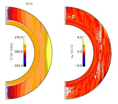
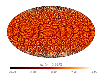
Figure 3: Same than Fig. 2 for the model M1b. In this case the vertical domain extends up to $r=0.985R_{\odot}$.

In order to include two different convection regimes (one dominated by rotation and another dominated by buoyancy) in the convection zone of our model, we extend the domain in the radial direction up to $r=0.985R_{\odot}$ and add a third layer with the polytropic index slightly smaller than the one in the convection zone, $m_{1}=1.4999$. Thus, the ambient state $\Theta_{e}$ decreases faster (increasing superadiabaticity) in the upper 5% of the domain (compare dotted line in Fig. 3a and b).

In Fig. 3 we present the differential rotation and meridional circulation profiles for this model (case  M1b). The rotation profile is similar to the case  M1, however in this case $\Delta\Theta$ is only $\simeq 30$ nHz. The meridional flow exhibit multiple cells. The radial velocity at the surface level shows broad convective structures at lower latitudes and small convection cells at middle and higher latitudes. The equatorial structures are still elongated in latitude, however the banana cells are not evident at this height. Like in the run  M1, they are evident at $r=0.96R_{\odot}$.

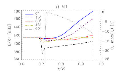
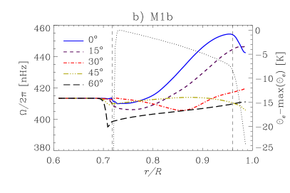
Figure 4: Radial distribution of the angular velocity for different co-latitudes. Left and right hand panels correspond to the models M1 and the M1b, respectively. A near surface shear layer appears for $r>0.96R$. The thin-dotted line corresponds to the radial distribution of $\Theta_{e}$ scaled with its maximum value.

In Fig. 4 we compare the radial distribution of differential rotation for the models without (M1) and with (M1b) this additional layer. Although the radial profiles of differential rotation for the case  M1b slightly differ from that without the upper layer ( M1), negative shear at lower latitudes is clearly observed (similar results were found by [Käpylä et al. (2011), Käpylä et al., 2011] in simulations with a large density contrast between the bottom and top of the domain). We notice that the radial component of the Reynolds stress tensor is also negative at these latitudes. However, our simulations are unable to capture the dynamics of the surface region and could not be extended above $r=0.985R_{\odot}$. An extended region of negative angular momentum flux might result in a pronounced poleward meridional flow near the surface, not observed here but present in the Sun. This meridional flow could transport angular momentum to higher latitudes and thus form a near-surface shear layer similar to the observations, as suggested by [Miesch & Hindman (2011)].

4 Conclusions

We have used the anelastic, hydrodynamic, version of the EULAG code to perform global numerical simulations of convection in a rotating stratified envelope and study different regimes of differential rotation. We consider first models with a bottom stable (subadiabatic) region and an extended convectively unstable layer. In these models we are able to reproduce previous results obtained with different codes. Different correlations between the turbulent velocities (Reynold stresses) are found for models with different rotation rates. These correlations appear as the competition between buoyancy and Coriolis forces and give rise to different mean flows patterns. Models in which convective velocities dominate over the rotation velocity result in profiles of the angular velocity with the equator rotating slower than higher latitudes. Models in which rotation dominates result in a faster equator and slower poles. For all models the bottom, convectively stable, layer rotates uniformly forming a region of strong rotational shear (tachocline) at the base of the convection zone. Unlike the Sun in all the models the rotation contours are mainly aligned along the rotation axis (cylindrical) following the Taylor-Proudman theorem.

We have also run simulations for models with higher numerical resolution, and obtained the mean flow profiles somewhat different from the lower resolution base model (L1). Paradoxically, the model with the coarse grid resembles better the solar rotation profile than the models with finer grids. This emphasizes the importance of the balance between the efficiency of convective mixing at resolved scales, the implicit eddy viscosities and the large scale forcing.

Finally, to model the fast convective motions at the top of the convection zone, we have added a third layer in the top of the domain where the potential temperature (entropy) declines quickly (corresponding to an increase of super adiabaticity). This layer generates convective motions with smaller spatial and temporal scales less affected by rotation than the deeper slow motions. In this model a near surface shear layer is formed at lower latitudes due to the negative radial transfer of the angular momentum.

Acknowledgements We thank P. Charbonneau and J-F Cossette for their important help in the construction of the spherical model. GG acknowledges NSF for travel support. All the simulation here were performed in the NASA cluster Pleiades.

References

- [Brandenburg (2005)] Brandenburg, A. 2005, ApJ, 625, 539
- [DeRosa et al. (2002)] De Rosa, M. L., Gilman, P. A. and Toomre, J. 2002, ApJ, 581, 1356
- [Domaradzki et al. (2003)] Domaradzki, J. A., Xiao, Z. and Smolarkiewicz, P. K. 2003, Phys. Fluids, 15, 3890
- [Gilman (1977)] Gilman, P. A., 1977, GApFD, 8, 93
- [Guerrero & de Gouveia Dal Pino (2008)] Guerrero, G. and de Gouveia Dal Pino, E. M., 2008, A&A, 485, 267
- [Guerrero & Käpylä (2011)] Guerrero, G. and Käpylä, P. J. 2011, A&A, 533, A40
- [Guerrero et al. (2013)] Guerrero, G., Smolarkiewicz, P. K., Kosovichev. A. and Mansour, N. 2013, ApJ, in preparation
- [Ghizaru et al. (2010)] Ghizaru, M., Charbonneau, P. and Smolarkiewicz, P. K. 2010, ApJL, 715, L133
- [Jouve & Brun (2007)] Jouve, L. and Brun, A. S. 2007, A&A, 474, 239
- [ Käpylä et al. (2011)] Käpylä , P. J., Mantere, M. J., Guerrero, G., Brandenburg, A., Chatterjee, P. 2011, A&A, 531, A162
- [ Käpylä et al. (2011)] Käpylä , P. J., Mantere, M. J., and Brandenburg, A., 2011, AN, 322, 883
- [Lipps & Hemler (1982)] Lipps, F.B. and Hemler, R.S., 1982, J.Atmos.Sci. 39, 2192
- [Lipps (1990)] Lipps, F.B., 1990, J.Atmos.Sci. 47, 1794
- [Margolin & Rider (2002)] Margolin, L. G. and Rider, W. J., 2002, IJNMF, 39, 821
- [Miesch et al. (2006)] Miesch, M. S. and Brun, A. S. and Toomre, J., 2006, ApJ, 641, 618
- [Miesch & Hindman (2011)] Miesch, M. S. and Hindman, B. W. 2011, ApJ, 743, 79
- [Pipin & Kosovichev (2011)] Pipin, V. V. and Kosovichev, A. G., 2011, ApJ, 741, 1
- [Prusa et al. (2008)] Prusa, J. M., Smolarkiewicz, P. K. and Wyszogrodzki, A. A., 2008, Comput. Fluids, 37, 9, 1193
- [Racine et al. (2011)] Racine, É., Charbonneau, P., Ghizaru, M., Bouchat, A. and Smolarkiewicz, P. K. 2011, ApJL, 735, 46
- [Smolarkiewicz et al. (2001)] Smolarkiewicz, P.K. Margolin, L.G. and Wyszogrodzki, A.A., 2001, J.Atmos.Sci, 58, 349
- [Smolarkiewicz (2006)] Smolarkiewicz, P.K., 2006, IJNMF, 50, 1123
- [Smolarkiewicz & Margolin (2007)] Smolarkiewicz, P.K. and Margolin, L.G., 2007, Implicit Large Eddy Simulation: Computing Turbulent Fluid Dynamics, Cambridge University Press, 2007, 413