Weighted -minimization for generalized non-uniform sparse model
Abstract
Model-based compressed sensing refers to compressed sensing with extra structure about the underlying sparse signal known a priori. Recent work has demonstrated that both for deterministic and probabilistic models imposed on the signal, this extra information can be successfully exploited to enhance recovery performance. In particular, weighted -minimization with suitable choice of weights has been shown to improve performance in the so called non-uniform sparse model of signals. In this paper, we consider a full generalization of the non-uniform sparse model with very mild assumptions. We prove that when the measurements are obtained using a matrix with i.i.d Gaussian entries, weighted -minimization successfully recovers the sparse signal from its measurements with overwhelming probability. We also provide a method to choose these weights for any general signal model from the non-uniform sparse class of signal models.
I Introduction
Compressed Sensing has emerged as a modern alternative to traditional undersampling for compressible signals. Previously, the most common way to view recovery of signals from samples was based on the Nyquist criterion. According to the Nyquist criterion, a band-limited signal has to be sampled at a rate at least twice its bandwidth to allow exact recovery. In this case the band-limitedness of the signal is the extra known information that allows us to reconstruct the signal from compressed measurements. In compressed sensing the additional structure considered is that the signal is sparse with respect to a certain known basis. As opposed to sampling at Nyquist rate and subsequently compressing, we now obtain linear measurements of the signal and the compression and measurement steps are now combined by obtaining much smaller number of linear measurements than what would be in general required to reconstruct the signal from its measurements.
After fixing the basis with respect to which the signal is sparse, the process of obtaining the measurements can be written as where, is the vector of measurements, is the signal and represents the linear functionals acting on the signal . We call the measurement matrix. The signal is considered to have at most non-zero components and we are typically interested in the scenario where is much smaller than . Compressed Sensing revolves around the fact that for sparse signals, the number of such linear measurements needed to reconstruct the signal can be significantly smaller than the ambient dimension of the signal itself. The reconstruction problem can be formulated as finding the sparsest solution satisfying the constraints imposed by the linear measurements . This can be represented by
| subject to |
This problem is inherently combinatorial in nature and is in general a NP-hard problem. This is because for a certain value of the size of the support of given by , one needs to search through all possible supports of the signal. Seminal work by Candés and Tao in [1] and Donoho in [2] show that under certain conditions on the measurement matrix , norm minimization, which can be recast as a linear program, can recover the signal from its measurements. Additionally, a random matrix with i.i.d. Gaussian entries with mean zero satisfies the required condition with overwhelming probability. Linear programming is known to have polynomial time complexity and the above mentioned result tells us that for a large class of measurement matrices we can solve an otherwise NP-hard combinatorial problem in polynomial time. Subsequently, iterative methods based on a greedy approach were formulated which recover sparse signals from their measurements by obtaining an increasingly accurate approximation to the actual signal in each iteration. Examples of these include CoSaMP [3] and IHT [4]. The compressed sensing framework has also been generalized to the problem of recovering low rank matrices from compressed linear measurements represented by linear matrix equations [5] [6].
Most of the earlier literature on Compressed Sensing focused on the case where the only constraints on the signal are those imposed by its measurements . On the other hand it is natural to consider the case where besides sparsity, there is certain additional information on the structure of the underlying signal. This is true in several applications, examples of which include encoding natural images (JPEG), MRI and DNA microarrays [7], [8]. This leads us to Model Based Compressed Sensing where the aim is to devise recovery methods specific to the signal model at hand. Furthermore, one would also want to quantify the possible benefits it has over the standard method (e.g. lesser number of required measurements for the same level of sparsity of the signal). This has been explored in some recent papers. The authors in [9] analyzed a deterministic signal model, were the support of the underlying signal is constrained to belong to a given known set. This defines a subset of the set of all -sparse signals, which is now the set of allowable signals. This results in an additional constraint on the original reconstruction problem.
| subject to | |||
It was shown that an intuitive modification to the CoSaMP or IHT method succeeds in suitably exploiting the information about the model. The key property defined in [1], known as the Restricted Isometry Property was adapted in [9] to a model based setting. With this, it was shown that results similar to [1] can be obtained for model-based signal recovery.
As opposed to this, a probabilistic model, i.e. a Bayesian setting, was considered in [10]. Under this model there are certain known probabilities associated with the components of the signal . Specifically, with are such that
The deterministic version of the same model called the “nonuniform sparse model” was considered in [11]. For this, the use of weighted -minimization was suggested, given by
| subject to |
where denotes the weighted norm of . The quantities are some positive scalars. Similar to [2], [12], ideas based on high dimensional polytope geometry were used to provide sufficient conditions under which weighted -minimization recovers the sparse signal. This method was introduced earlier in [13] where it was used to analyze the robustness of -minimization in recovering sparse signals from noisy measurements. The specific model considered in [10] can be described as follows. Consider a partition of the indices to into two disjoint sets and . Let and . As a natural choice choose the weights in the weighted -minimization as and . The main result of [10] is that under certain conditions on , and , weighted -minimization can recover a signal drawn from the above model with overwhelming probability. This was later extended in [11] to the case when the support of the sparse signal is divided into classes, where is a fixed constant, see Theorem 5.3 in [11].
In this paper, we consider a generalization of the non-uniform sparse model with mild assumptions. In particular, we keep the assumption that each element of the sparse signal has a probability of being non-zero independent of every other element. To describe the behavior as , we assume that these probabilities converge to some shape function i.e.,
| (1) |
Assumption 1.
The probability shape function satisfies the following conditions:
-
(a)
is continuous in except at finitely many points.
-
(b)
Within each interval that is continuous, it is monotonically non-increasing.
The above assumptions are mild and many shape functions with finitely many discontinuities can be “rearranged” to satisfy the second assumption.
The possibility of specifying a non-uniform probability shape function can be useful in several applications. For example, natural images often have sparsity properties after certain transforms, including the Fourier and wavelet transforms. Furthermore, they tend to have significantly more content in the lower frequencies, which causes a natural decay in the likelihood of non-zero Fourier coefficients with increasing frequencies. This decay can then be modeled as the shape function described above. In the context of specific applications, this information can be deduced, for instance, from the statistics of previous training data.
For a signal drawn from this model, we propose the use of weighted -minimization to reconstruct it from its compressed linear measurements, and in addition, to match the signal model, we propose that the weights be chosen according to a shape function which satisfies the same properties as , except that it is monotonically non-decreasing instead. Note that, we have still kept the independence assumption, which does not take into account for example correlations in the signal support. However, weighted -minimization is generally not a suitable choice in that case which is why we do not consider such correlations in our model.
We prove that under certain conditions on , and the measurement matrix , we can reconstruct the signal perfectly with overwhelming probability. Although a good part of the machinery in [2] and [11] applies to our case, difficulties arise because of the generality of the class of functions described above. In addition to computing the usual angle exponents, typical of the high-dimensional geometry based analysis in [2], we also need to investigate further properties of these exponents with respect to the weight function , such as monotonicity, in order to compute a true upper bound on the probability of failure. Additionally, to make sure that the angle exponents, which are described as the solution to an optimization problem, can be efficiently computed numerically, we prove their partial convexity with respect to the optimizing variables. The angle exponent analysis along with the monotonicity and partial convexity properties help us formulate and prove sufficient conditions for sparse signal recovery that also allow efficient numerical verification.
A major question that arises in our general setting, is how to choose the function for the weighted -minimization according to . We answer this question by providing a definitive recommendation for the choice of weights based on Gaussian width computations using Gordon’s theorem. This, along with our angle exponent analysis, which is generally known to be quite tight, provides a general framework for designing a weighted -minimization based recovery method as well as a way to verify its performance theoretically for the non-uniform sparse model.
The rest of the paper is organized as follows. In Section II, we introduce the basic notation. We formulate the exact questions that we set out to answer in this paper and state our main theorem. In Section III we focus on how weighted -minimization behaves by restricting our attention to special class of signals that are particularly suitable for the ease of analysis. We later show that the methods generalize to other simple classes and is all we need to establish the main result of this paper. In Section IV we describe the key features of a typical signal drawn from our model. We also prove a suitable large deviation result for the probability that a signal drawn from our model lies outside this typical set. In Section V, we provide a method for deriving a recommended weight function based on minimizing an upper bound on Gaussian width. In Section VI we provide numerical computations to demonstrate the results we derive and then provide simulation results. We conclude the paper in Section VII.
II Problem Formulation
II-A Notation and parameters
We denote scalars by lower case letters (e.g. c), vectors by bold lower case letters (e.g. x), matrices with bold upper case letters (e.g. A). Probability of an event E is denoted by . The standard unit vector in is denoted by , where the “” is located in the position.
The underlying sparse signal is represented by , the measurement matrix by . The vector of observations is denoted by and is obtained through linear measurements of given by . Typically we would need linear measurements to be able to recover the signal. The scalar determines how many measurements we have as a fraction of . We call this the compression ratio.
II-B Model of the Sparse Signal
Let be a continuous monotonically non-increasing function. We call the probability shape function and the reason for this name will become clear from the description below. The support of the signal is decided by the outcome of independent Bernoulli random variables. In particular, if denotes the event that , then the events are independent and . Although we assume throughout the paper that is continuous, our result generalizes to piecewise continuous functions as well. Let us denote by the cardinality of . Note that under the above model is a random variable that can take any value from to . The expected value of is given by . We denote by the expected fractional sparsity given by .
We notice here that the signal model described above is much more restrictive than the ones made in Assumption 1. However, as it turns out, the exact same analysis also works for the more general case in Assumption 1, so we stick to the simplified model above to keep the notation and analysis less cumbersome.
As is standard in Compressed Sensing literature we assume that the entries of the measurement matrix are i.i.d. Gaussian random variables with mean zero and variance one. The measurements are obtained as .
II-C Weighted -minimization
When the fractional sparsity is much smaller than one, a signal sampled from the model described above is sparse. Hence, it is possible to recover the signal from its measurements by -minimization which is formulated as
| subject to |
However this does not exploit the extra information available from the knowledge of the priors. Instead, we use weighted -minimization to recover the sparse signal which is captured by the following optimization problem:
| (2) | ||||
| subject to |
where is a vector of positive weights and refers to the weighted norm of , for a given weight vector . The weight vector plays a central role in determining whether (2) successfully recovers the sparse signal . Intuitively, should be chosen in a certain way depending on so as to obtain the best performance (although at this point we have not precisely defined the meaning of this). Keeping in mind the structure of , we suggest using weights which have a similar structure. Formally, let be a non-negative non-decreasing continuous function. Then we choose the weights as . We call the weights shape function.
II-D Problem statement
In this paper we try to answer the following two questions:
-
•
Given the problem parameters (size of the matrix defined by ), the functions and , does weighted -minimization in (2) recover the underlying sparse signal with high probability?
-
•
Given a family of probability shape functions , how to choose the weight function that has the best performance guarantees? Here is the expected sparsity of the model.
We give an answer in the affirmative to the first question, given that the functions and satisfy certain specified conditions. This is contained in the main result of this paper which is
Theorem 1.
Let the probability shape function and the weight shape function be given. Let E be the event that weighted -minimization described in (2) fails to recover the correct sparse vector . There exists a quantity which can be computed explicitly as described in Appendix B-4, such that whenever the probability of failure of weighted -minimization decays exponentially with respect to . More precisely, if for some we have . then there exists a constant such that for large enough , the probability of failure satisfies .
To answer the second question, we need to define the measure of performance. For a given value of , let
| (3) | ||||
| subject to | (4) |
We call the guaranteed bound on recoverable sparsity . In Section V, we answer the question of choosing the best , and in Section VI we use numerical computations to demonstrate that this choice indeed outperforms other natural choices when we compare the attained by each choice.
III Analysis of Weighted -minimization
In this section, we analyze the performance of weighted -minimization with weights specified by on a certain special class of sparse signals . As we will see in Section IV, we can easily generalize the analysis to the signals drawn from our signal model.
Recall that the failure event from Theorem 1 is defined as the event that weighted -minimization fails to recover the correct sparse vector . We call the probability of this event as the probability of failure. Without loss of generality we can assume that , that is lies on a -dimensional face of the weighted cross-polytope
which is the weighted -ball in dimensions. The specific face of on which lies is determined by the support of . The probability of failure can be written as
where is the set of all faces of the polytope . Then, as shown in [10], the event is precisely the event that there exists a non-zero such that conditioned on . Also since has i.i.d. Gaussian entries, sampling from the null space of is equivalent to sampling a subspace uniformly from the Grassmann manifold . So conditioned on the event is same as the event that a uniformly chosen -dimensional subspace shifted to intersects the polytope at a point other than . The probability of the above event is also called the complementary Grassmann Angle for the face with respect to the polytope under the Grassmann manifold . Based on work by Santaló [14] and McMullen [15] the Complementary Grassmann Angle can be expressed explicitly as the sum of products of internal and external angles.
| (5) |
where and are the internal and external angles and is the set of all -dimensional faces of . The definitions of internal and external angles can be found in [10]). We include them here for completeness.
-
•
The internal angle is the fraction of the volume of the unit ball covered by the cone obtained by observing the face from any any point in face . The quantity is defined to be zero if is not contained in and is defined to be one if . In Figure 1, if the face is the vertex and the face is the face formed by , then as labelled.
-
•
The external angle is defined to be the fraction of the volume of the unit ball covered by the cone formed by the outward normals to the hyperplanes supporting at the face . If then is defined to be one. In Figure 1, if is the edge , then the external angle as labelled. The ray is orthogonal to the face and the ray is orthogonal to the face , i.e., normals to the supporting hyperplanes of .

In this section we describe a method to obtain upper bounds for by finding upper bounds on the internal and external angles described above. We first analyze for the “simplest” class of faces. We denote by , the face whose vertices are given by . Thus the vertices are defined by the first indices and we call this face the “leading” -dimensional face of . We will spend much of this section developing bounds for for such “leading” faces. Then in Section IV, we describe the typical set of our signal model and show that for the purposes of bounding it is sufficient to consider a certain special class of faces. The bounds we develop in this section for “leading” faces can be easily generalized to faces belonging to this special class.
III-A Angle Exponents for leading faces
We define the family of leading faces as the set of all faces whose vertices are given by for some . In this section we will establish the following result which bounds the internal and external angles related to a leading face of . We will then use this result in the next section to provide an upper bound on for .
Theorem 2.
Let and with . Let be the face whose vertices are given by and let be the face whose vertices are given by . Then there exist quantities and which can be computed explicitly as described in Section III-C2 and Section III-C3 respectively, such that for any , there exist integers and satisfying
-
•
, for all ,
-
•
, for all .
The quantities and are called the optimized internal angle exponent and the external angle exponent respectively.
Whenever any of the angle exponents described above is negative, the corresponding angle
decays at an exponential rate with respect to the ambient dimension . We will prove Theorem 2 over the following two
subsections by finding the optimized internal and external angle exponents that satisfy the requirements of the theorem.
III-A1 Internal Angle Exponent
In this subsection we find the optimized internal angle exponent that satisfies the conditions described in Theorem 2. We begin by stating the following result from [10] which provides the expression for the internal angle of a face with respect to a face in terms of the weights associated with their vertices. Subsequently, we find an asymptotic upper bound on the exponent of the internal angle using that expression. In what follows, we denote by the distribution of a half normal random variable obtained by taking the absolute value of a distributed random variable.
Lemma 1.
[10] Define Let be a normal random variable and for be independent half normal distributed random variables that are independent of . Define the random variable . Then,
where is the density function of .
We now proceed to derive an upper bound for the quantity . Much of the analysis is along the lines of [2]. Let the random variable be defined as . So, and using the convolution integral, the density function of can be written as
where is the cumulative distribution function of . Let be the mean of the random variable . Then,
As in [2], the second term satisfies . As we will see later in this section for some and hence . Since we are interested in computing the asymptotic exponent of , we can ignore from this computation. To bound , we use , where denotes the rate function (convex conjugate of the characteristic function ) of the random variable . So we get
| (6) |
For ease of notation we define the following quantities.
Here is the characteristic function of the standard half normal random variable and is the standard normal distribution function. Using the above definition, we can express the relation between and as
We compute
Changing variables in (6) by substituting , we get
Now, as , we have
Define . This gives us . Similarly,
where is defined as . This gives us
where is defined as . Using Laplace’s method to bound as in [2], we get
| (7) |
where and is the minimizer of the convex function . Let
Then the maximizing satisfies From convex duality, we have . The minimizing of satisfies
| (8) |
This gives
| (9) |
First we approximate as follows
From the above we obtain
Combining this with equation (9), we can determine up to a error by finding the solution to the equation
| (10) |
We define the internal angle exponent as
| (11) | ||||
| (12) |
and the optimized internal angle exponent as
| (13) | ||||
| (14) | ||||
| (15) |
where is determined through from equation (8) and is determined by solving the equation (10). From inequality (7)
and Lemma 1 we
see that the function satisfies the conditions described in the first part
of Theorem 2.
III-A2 External Angle Exponent
In this subsection we find the optimized external angle exponent that satisfies the statement of Theorem 2. We proceed similar to the previous section and begin by stating the following lemma from [10] which provides the expression for the external angle of a face with respect to the polytope in terms of the weights associated with its vertices. We then find an upper bound on the asymptotic exponent of the external angle.
Lemma 2.
[10] The external angle is given by
To simplify the expression for the external angle, we define the standard error function as
and rewrite the external angle as
Similar to the method used in the previous section
where is defined as . Substituting this we have
where is defined as . Again using Laplace’s method we get
| (16) |
where is the minimizer of and . The minimizing satisfies where
We first approximate as follows:
So the minimizing can be computed up to an error of by solving the equation
| (17) |
We define the external angle exponent as
| (18) |
and the optimized external angle exponent as
| (19) | |||
| (20) |
where can be obtained by solving equation (17).
III-B Recovery Threshold for the family of leading faces
In this section we use the bounds on the asymptotic exponents of the internal and external angle from Theorem 2 to find an upper bound for for . The main result of this section is the following theorem.
Theorem 3.
Let for . be the face with . There exists a function which we call the total exponent of such that given , there exists such that for all , . The function can be computed explicitly as described in (21).
Using the decomposition equation (5) and the fact that is non-zero only if , we get
Recall that is the set of all -dimensional faces of .
To proceed, we will need the following useful lemma (proof can be found in the appendix).
Lemma 3.
Among all -dimensional faces of satisfying , the face that maximizes and is the one with as its vertices.
Using Lemma 3, we get
Using , and Stirling’s approximation for factorials, it can be shown that
where is the entropy function with base defined by . Define the combinatorial exponent as
So, we conclude,
The function defined by
satisfies the condition given in Theorem 3, and hence establishes the theorem.
III-C Obtaining tighter exponents
In Section III-B, we developed a method that provides an upper bound on in terms of internal and external angle exponents. For a given value of , we bounded and for each by by using Lemma 3. This bounding step is generally rather overly conservative because it does not take into account the variation of the function over the complete interval . The quality of bound is especially poor for choices of function which are rapidly increasing. To improve on the bound, we can use a simple technique which allows us to take into account the variation of with respect to more accurately over the whole interval.
Divide the set of indices into two parts with and . For a particular , let have vertices in and vertices in . Using Lemma 3, among all faces with the values of and specified as above, the choice that maximizes and is the face with vertices given by the indices . Using this we get a revised upper bound on
Define and . Then the revised bound on the exponent of can be obtained as
where we define and call it the combinatorial exponent The expressions for and are can be obtained by using the methods of the previous subsection (we will give the exact expressions shortly). The function
now satisfies the role of the total exponent in Theorem 3.
We can repeat the above argument for any by dividing the indices denoted by into parts. Define the quantities as where is the number of indices of face in the interval. Also define and let . The total exponent is now given by
| subject to |
where
The dependence of the exponent functions on other variables has been suppressed for compactness.
So, the total exponent can be obtained by the following maximization:
| (21) | ||||
| subject to |
We now compute the expressions for each of the functions appearing in the above maximization.
For the subsequent derivation, we define .
III-C1 Combinatorial Exponent
The combinatorial exponent is given by
For the internal and external angle exponents, in addition to obtaining their expressions, we will also bound them suitably by analytically simpler expressions so that the
optimization problem described in (21) becomes more tractable.
III-C2 External Angle Exponent
We start with
where
As is an increasing function, the integral appearing above in the expression of can be bound by its left Riemann sum.
Similary,
So,
Combining we obtain a simplified expression for the external angle exponent as
The optimized external angle exponent is then given by
III-C3 Internal Angle Exponent
We start with
where
is the convex conjugate of and is given by,
We are interested in only in the region . In this region we have,
which follows from the fact that and is an increasing function of . This gives
and hence
So, we conclude
From the above we obtain a simplified expression for the internal angle exponent as
The optimized internal angle exponent is then obtained as
To show that the maximization with respect to in (21) can be performed efficiently, we will show that is a concave function of for fixed value of and . This follows from the following lemma. The proof can be found in the appendix.
Lemma 4.
The combinatorial, internal and external angle exponents are concave functions of for fixed values of and .
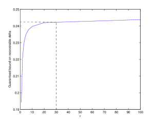
The parameter which governs the number of evaluation points we use to compute the angle exponents gives us a method to control the accuracy of the computed exponents. If we can obtain a value such that for all we have , then Theorem 3 guarantees that whenever , weighted -minimization recovers the corresponding sparse signal with overwhelming probability. We call this the guaranteed bound on recoverable sparsity levels . Increasing results in a tighter guaranteed bound but at the expense of an increased cost in performing the optimization in (21). In Figure 2 we show via simulation how this bound improves with the parameter . For this, we fix a compression ratio . The weights are chosen as which corresponds to the weight function . Note how the bound improves with increasing value of but saturates quickly. This indicates that a moderately large value of (e.g. from the figure) will suffice for accurate enough angle exponent computations.
IV Proof of Theorem 1
In this section, we establish the main result of this paper which is Theorem 1. We do this in two steps. We first characterize the properties of a typical signal drawn from our model and provide a large deviation result on the probability that a signal drawn from our model does not satisfy this property. For signals which have this typical property, we then use the analysis method of Section III to find the exponent in the statement of Theorem 2. We start by writing
To analyze this expression we will further split the sum into faces belonging to different “classes” which we describe below. Divide the set of indices from into equal parts with denoting the interval of indices. Any face of the skewed cross polytope can be fully specified by the index of its vertices (up to the signs of the vertices). For a given face , let the set of indices representing the face be denoted by . For a given denote by , the set of all faces of with . Also let . Recall that we denote by the failure event, i.e. the event that the weighted -minimization does not produce the correct solution. Then we have
| (22) |
We can just consider one representative among the faces created by the different sign patterns. This is because, by the symmetry of the problem, all the faces have the same probabilities and . For simplicity we always choose this representative as the face that lies in the first orthant.
The function is an increasing function of for . So,
Denote the right hand side of the above inequality be , which means for we have . Define
Then
By Lemma 3, among all faces , the one which maximizes is the one obtained by stacking all the indices to the right of each interval. We denote this maximum probability by . Combining the above we get
| (23) |
As the function is monotonically decreasing, is not same for all . We now proceed to show that is significant only when takes values in a “typical” set. For values of outside the typical set is exponentially small in and can be ignored in the sum in (23). For in the typical set, we will use the methods of Section III to bound and hence .
The following Lemma provides bounds for which will motivate the definition of typicality that follows.
Lemma 5.
Let denote the Kullback-Leibler distance between two Bernoulli random variables with probability of success given by and respectively. Define . If we have , then there exists , such that for all ,
where is a positive constant.
Proof.
We have
Then,
Letting ,
where is the error in the Riemann sum given by . Now further divide each of the intervals into equal parts thus forming a total of intervals. Let denote the number of indices of face in the interval counted according to the new partition. Summing up the number of indices in all the intervals of length contained in an interval of length gives . Also let . The calculations just carried out above can be repeated for this new partition to give
We now bound the term .
Using the log-sum inequality, we obtain,
where, . Using this,
Since this is true for every , we let to get
So, if the condition of the lemma is satisfied, then
and the claim in the lemma then follows. ∎
Lemma 5 motivates the following natural definition of -.
Definition 1.
Given , define to be -typical if .
Using this definition of -, we can now bound the probability of failure by using (23) as
For a fixed value of , the number of possible values of is bounded by . Since , the second term can be bounded as
for some positive constant . As , there exists , such that for all ,
for some positive constant . This allows us to only consider the first term for which are -typical. Among all -, let be the face which maximizes the probability . Then,
This gives
Also, since we can choose to be as small as we want, we can essentially just consider the case with . This gives us with . This defines a fixed face which we call the typical face of and we only need to bound the term which can be done by a simple generalization of the methods in Section III. The corresponding expressions for the optimized internal and external angle exponents can be found in the Appendix.
V Choosing the weight function
In this section, we provide a method for choosing the weight function used in the weighted -minimization based on the probability function . For a given function , the aim is to find a function which provides the best recovery guarantees defined in (4).
A natural way to choose the best function would be to minimize the total exponent with respect to . The recovery thresholds obtained from the angle exponent based analysis used in Section III is known to be quite accurate in practice. For our specific case, we provide further evidence of this fact in Section VI via simulations. However, one disadvantage of this method is that the dependence of the recovery threshold on the functions and is not very intuitive, making it difficult to find the optimal for a given . In this section, we take an alternative approach based on estimating the Gaussian width of the cone of feasible directions of the (weighted) polytope using Gordon’s theorem [16] . This method was first introduced in [17] in the context of sparse signal recovery. It was later used by [18], where it was used to obtain, among other quantities of interest, the weak recovery threshold for the standard -minimization. This threshold matched the one obtained in [2] indicating that it is tight. However, to achieve this tightness, the computations used are quite involved and it is not clear how it may be extended to analyze weighted -minimization, especially in a fairly general setting like ours. Instead, we use the analysis in [19], which sacrifices some tightness but leads to very amenable expressions showing the dependence on and .
Before we begin, we first introduce some notation and state a few useful results from [19] that we use in our analysis. Let be the underlying sparse vector normalized as before such that . Let the cone be defined by . Let , where is the sphere in dimensions. The Gaussian width of is defined as
where the expectation is taken over . The following corollary of Gordon’s theorem is stated in [19].
Corollary 1.
[19] If , then weighted -minimization recovers the correct underlying sparse vector with probability at least . Here is the expected length of a -dimensional Gaussian vector.
Since, we want to find weights which minimize the exponent in the probability of failure, in turn we should try to minimize the Gaussian width .
The following lemma proved in [19] will help us simplify the computations needed to estimate the Gaussian width .
Lemma 6.
[19] Let denote the polar of the cone . Then .
The first inequality in the above lemma is based on a duality argument and it is remarked in [18] that it is tight, i.e., strong duality holds. The second inequality is a direct application of Jensen’s inequality. From here, we proceed to compute an upper bound on the Gaussian width along the lines of [19]. The cone is given by
So,
where is the shrinkage function given by
Hence for all ,
| (24) | ||||
| (25) | ||||
| (26) |
Recall from Section IV that, if we divide the indices into equal parts , then we can assume that the support of the underlying sparse vector drawn according to has elements in , where . Using this and the fact that is monotonically increasing in , we get from (26),
We seek to find that minimizes . Since we are interested in the asymptotics as , we can choose large to obtain
Note that replacing by does not change the weighted -minimization and hence we can drop in the above expression. The optimal choice of is obtained by
| (27) |
For a given choice of , is a convex function of and the above minimization can be efficiently performed numerically. This defines a one to one map between the probability function and the corresponding weight function .
The method used in this section relies on minimizing an upper bound on the error exponent, which in turn leads to a justifiable prescription for choosing the weight function . Once such an is obtained, we can then use the angle exponent based analysis of Section III to verify the performance of this choice of for the given probability function .
VI Numerical computations and simulations
In this section, we compute the bounds using the techniques developed in this paper for a specific probability function . In particular we choose to be a linear function whose slope is governed by a parameter :
| (28) |
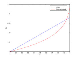
The expected level of sparsity of signals drawn from this model is . The value of governs how tilted the signal model is. Larger values of results in a higher tilt which means a random signal drawn from this model will have most of its non-zero entries concentrated at the beginning. To recover signals drawn from this model we use weighted -minimization with choice of weights defined by the weight function chosen to be one of the following:
-
(i)
-
(ii)
The recommended choice of given in (27).
The reason for choosing the linearly parameterized family of functions in item is twofold. One, it is a simple natural choice of a parameterized family of weights that may be chosen to match the probability function in (28), and this provides a basis for comparing the theoretical performance of this natural choice with the recommended choice (27). Second, it allows us to demonstrate how to use the methods described in this paper for computing the total exponent to choose the “best” weight function from a given parameterized family for a specific probability function . Recall from (4) the quantity
| subject to | (29) |
which is called the guaranteed bound on recoverable sparsity .
Before proceeding to evaluation of the performance of weighted -minimization in the problem specified by the above choice of functions, we will first present theoretical bounds and simulations related to the behavior of the so-called family of leading faces , when the corresponding cross-polytope is described by the function . This is contained in Section VI-A. The reader interested in the performance of weighted -minimization can skip over to Section VI-B.
VI-A Behavior of the leading family of faces under random projection.
Recall that, for a given set of weights, the weighted -ball is the cross polytope in dimensions whose vertices in the first orthant are given by for some . We call this face . In Section III-B, we developed sufficient conditions when weighted -minimization recovers a signal whose support is the first indices with overwhelming probability whenever . Similar to (29), we can define a corresponding specific to the family of leading faces given by
| subject to |
where is the total exponent for the face with as defined in (21). From the above definition and Theorem 1, it can be concluded that whenever , we are guaranteed to be able to recover the corresponding sparse signal with overwhelming probability. We call the quantity to be the guaranteed bound on recoverable sparsity levels . In view of our choice of weights, which is described by the function with , higher values of correspond to more steeply varying weights. Intuitively, one may expect that higher values of , will make the weighted norm cost function favor non-zero entries in the first few indices which may allow the threshold to be larger.
We will show that the quantity follows an increasing trend as described above. To demonstrate this for a certain choice of the parameters, we fix the compression ratio and compute the bound using the methods developed in Section III-B. Based on Figure 2 we choose as a reasonable value for the accuracy parameter in our computations. Figure 3 shows the dependence of this threshold on the value of which governs the weight function . The value of the bound at corresponds to the case when is a face of the regular ball. This is the threshold for below which standard -minimization succeeds in recovering a signal with sparsity level with overwhelming probability. As expected this value matches the value reported earlier in [2].
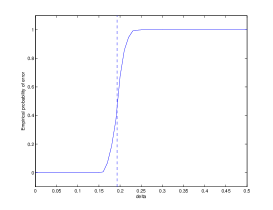
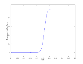
To evaluate the accuracy of the bound, we then compare the values of the threshold predicted by the guaranteed bound to that obtained empirically through simulations for two different values of the parameter . For this, we set , and obtain the fraction of times failed to be recovered correctly via weighted -minimization from a total of 500 iterations. This is done by randomly generating a vector for each iteration with support and using weighted -minimization to recover that from its measurements given by . Figure 4a and Figure 4b show this plot for and respectively. The vertical lines in the plots (marked A and B respectively) denote the guaranteed bounds corresponding to the value of in Figure 3. The simulations show a rapid fall in the empirical value of around the theoretical guaranteed bound as we decrease the value of . This indicates that the guaranteed bounds developed are fairly tight.
VI-B Performance of weighted -minimization.
In this subsection, we compute the theoretical bound on recoverable sparsity levels using the methods of this paper. We use the probability function in (28). We first start with the weight function in item (i). The choice of plays an important role in the success of weighted -minimization and it would be of interest to be able to obtain the value of for which one gets best performance. One way to estimate the effect of is to compute the guaranteed bound (29) as suggested in Section VI-A and observe the trend. We can then pick the value of which maximizes .
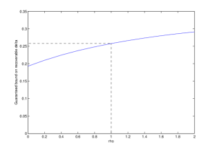
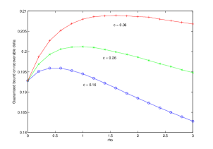
To demonstrate this via computations we fix the ratio and compute the guaranteed bound on recoverable (which denotes the expected fraction of non-zero components of the signal) using the methods developed in Section IV. The accuracy parameter is fixed at 60. Figure 5 shows the dependence of on the values of for three different values of . The curves suggest that for larger values of , which correspond to more rapidly decaying probabilities, the value of which maximizes is also higher. At the same time, the value of evaluated at also increases with increasing . This suggests that rapidly decaying probabilities allow us to recover less sparse signals by using an appropriate weighted -minimization.
Second, we compute the recommended choice of weight function by numerically solving for in (27) at the required evaluation points. We then compute the guaranteed bound defined in (29) by using this choice of weights. The parameters and are fixed at and as in the previous case above.
Comparing the values of from Table I and Table II, we can see that using the recommended choice of weight function does indeed have a larger guaranteed bound on recoverable sparsity for each of the choices of considered.
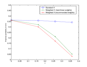
To provide evidence that weighted -minimization indeed improves performance, we conduct simulations to compare standard and weighted -minimization. We fix the value of to be . We then explore the effect of choosing different values of the model parameter in (28) on recoverability. We sample random signals with supports generated by the distribution imposed by . We then choose the weight function in two different ways. One by utilizing the curves computed in Figure 5 to make the best choice of (see Table I) and second by using the recommended choice from (27). We use weighted -minimization corresponding to these choice of weights to recover the generated signal from its measurements. We compute the fraction of the experiments for which this method fails to recover the correct signal over 500 experiments. The values of and are chosen to be and respectively. To compare the performance of weighted -minimization to standard -minimization, we repeat the same procedure but use standard -minimization to recover the signal. Figure 7 compares the values generated by each method. Notice how the performance of the standard -minimization method remains more or less invariant with increasing . This shows that standard -minimization fails to exploit the extra information present because of the knowledge of (i.e. the decaying nature of the probabilities) and its performance depends only on the value of , the expected fractional level of sparsity and is insensitive to the tilt of the model given by . On the other hand, the performance of weighted -minimization improves with for both choice of weight functions, with the recommended choice (27) showing the best performance.
.
| c | 0 | 0.16 | 0.26 | 0.36 |
|---|---|---|---|---|
| 0 | 0.6 | 1.0 | 1.6 | |
| 0.1928 | 0.1959 | 0.2012 | 0.2089 |
.
| c | 0 | 0.16 | 0.26 | 0.36 |
|---|---|---|---|---|
| 0.1928 | 0.1960 | 0.2014 | 0.2097 |
VII Conclusion
In this paper we analyzed sparse signal recovery via weighted -minimization for a special class of probabilistic signal model, namely when the weights are uniform samples of a continuous function. We leveraged the techniques developed in [2] and [10] to provide sufficient conditions under which weighted -minimization succeeds in recovering the sparse signal with overwhelming probability. In the process, we also provided conditions under which certain special class of faces of the skewed cross-polytope get “swallowed” under random projections.
A question central to the weighted -minimization based approach is the optimal choice of weights. In this paper, we provide a general framework to choose these weights. The recovery capacity of this choice of weights can also be verified theoretically by computing the angle exponents using the methods of this paper.
Appendix A proof of Lemmas 3 and 4
A-A Proof of Lemma 3
Let be the face whose vertices are given by . Let be any face other than whose vertices are given by . Consider forming a sequence of faces , where , and is obtained from by swapping the vertices and . Since , the expression in Lemma 2 for the external angle increases at each step. Hence, .
For a fixed value of , the exponent for the internal angle is only affected by the term in the expression for internal angle exponent in Lemma 1. Also
Following the same procedure as above for generating the sequence of faces , it can be seen that at each step the variance of some is decreased while keeping the other s unchanged. Thus in the above expression for increases at each step. Thus, the exponent for is greater than or equal to that of .
A-B Proof of Lemma 4
We rewrite the expression for the combinatorial exponent from Section III-C1:
The concavity of this function follows from the fact that the standard entropy function is a concave function. From its expression in Section III-C2 we observe that the external angle exponent is a linear function of and hence a concave function. The concavity of the internal angle exponent is slightly more involved and we spend the rest of this section in proving it.
The internal angle exponent as computed in Section III-C3 is given by
The quantity is a linear function of . So is a convex quadratic function of . Therefore it suffices to prove that is convex in . Recall that
Therefore
Since the argument in the above maximization is linear in it follows that is convex in .
Appendix B Angle exponents for the typical face
Divide the interval into equally spaced intervals. Let the face in consideration have indices in the interval. Also, let . The asymptotic exponents for this face can be obtained easily by a straight-forward generalization of the procedure described in Section III-A. We give the final expressions for the combinatorial, internal and external angle exponents for a given value of . In what follows, we use .
B-1 Combinatorial Exponent
where is the binary entropy function with base .
B-2 Internal Angle Exponent
The negative of the internal angle exponent is given by
where
Here is the characteristic function of the standard half-normal distribution.
B-3 External Angle Exponent
The negative of the external angle exponent is given by
where,
B-4 Total Exponent
Combining the exponents we define the total exponent as
| subject to | |||
where . From Theorem 3, the total exponent satisfies
So as long as the quantity , weighted -minimization succeeds in recovering the sparse signal with an exponentially small probability of failure.
References
- [1] E. Candès and T. Tao, “Decoding by linear programming,” IEEE Trans. on Information Theory, vol. 51, no. 12, pp. 4203–4215, December 2005.
- [2] D. Donoho, “High dimensional centrally symmetric polytopes with neighborliness proportional to dimension,” Discrete and Computational Geometry, vol. 102, no. 27, pp. 617–652, 2006.
- [3] D. Needell and J. A. Tropp, “CoSaMP: Iterative signal recovery from incomplete and inaccurate samples,” Appl. Comput. Harmon. Anal., vol. 26, no. 3, pp. 301–321, 2009.
- [4] T. Blumensath and M. E. Davis, “Iterative hard thresholding for compressed sensing,” Applied and Computational Harmonic Analysis, vol. 27, no. 3, pp. 265–274, 2009.
- [5] B. Recht, M. Fazel, and P. Parrilo, “Guaranteed minimum-rank solutions of linear matrix equations via nuclear norm minimization,” SIAM Review, vol. 52, no. 3, pp. 471–501, 2010.
- [6] B. Recht, W. Xu, and B. Hassibi, “Necessary and sufficient conditions for success of the nuclear norm heuristic for rank minimization,” Mathematical Programming, Series B, vol. 125, no. DOI 10.1007/s10107-010-0422-2, 2010.
- [7] W. Dai, M. Seikh, O. Milenkovic, and R. Baraniuk, “Compressive sensing DNA Microarrays,” EURASIP Journal on Bioinformatics and Systems Biology, 2009.
- [8] H.Vikalo, F. Parvaresh, S.Misra, and B.Hassibi, “Recovering sparse signals using sparse measurement matrices in compressed DNA microarrays,” IEEE Trans. on Signal Processing, special issue on genomic signal processing, vol. 2, no. 3, June 2008.
- [9] R. G. Baraniuk, V. Cevher, M. F. Duarte, and C. Hegde, “Model based compressive sensing,” IEEE Trans. on Information Theory, vol. 56, pp. 1982–2001, April 2010.
- [10] W. Xu, “Compressive sensing for sparse approximations: Construction, algorithms and analysis,” Ph.D. dissertation, California Institute of Technology, Department of Electrical Engineering, 2010.
- [11] M. A. Khajehnejad, W. Xu, A. S. Avestimehr, and B. Hassibi, “Analyzing weighted minimizaion for sparse recovery with nonuniform sparse models,” IEEE Trans. on Signal Processing, vol. 59, no. 5, pp. 1985–2001, 2011.
- [12] D. Donoho and J. Tanner, “Neighborliness of randomly-projected simplices in high dimensions,” Proc. National Academy of Sciences, vol. 102, no. 27, 2005.
- [13] W. Xu and B. Hassibi, “Compressed sensing over the Grassmann manifold: A unified analytical framework,” Allerton Conference, 2008.
- [14] L. A. Santaló, “Geometría integral en espacios de curvatura constante.” Rep. Argentina Publ. Com. Nac. Energía Atómica, Ser. Mat 1, No. 1, 1952.
- [15] P. McMullen, “Non-linear angle-sum relations for polyhedral cones and polytopes,” Math. Proc. Cambridge Philos. Soc., vol. 78, no. 2, pp. 247–261, 1975.
- [16] Y. Gordon, “On milman’s inequality and random subspaces with escape through a mesh in ,” Geometric aspects of functional analysis, Israel Seminar 1986 - 87, Lecture Notes in Mathematics, vol. 1317, pp. 84–106.
- [17] M. Rudelson and R. Vershynin, “On sparse reconstruction from Fourier and Gaussian measurements,” Communications on Pure and Applied Mathematics, vol. 61, no. 8, pp. 1025–1045.
- [18] M. Stojnic, “Various thresholds for optimization in comressed sensing,” arXiv, no. 0907.3666v1, 2009.
- [19] V. Chandrasekaran, B. Recht, P. Parrilo, and A. Willsky, “The convex geometry of linear inverse problems,” Foundations of Computational Mathematics, vol. 12, no. 6, pp. 805–849, 2012.