Characterization of the Optical and X-ray Properties of the Northwestern Wisps in the Crab Nebula

Abstract

We have studied the wisps to the north-west of the Crab pulsar as part of a multiwavelength campaign in the visible and in X-rays. Optical observations were obtained using the Nordic Optical Telescope in La Palma and X-ray observations were made with the Chandra X-ray Observatory. The observing campaign took place from 2010 October until 2012 September. About once per year we observe wisps forming and peeling off from (or near) the region commonly associated with the termination shock of the pulsar wind. We find that the exact locations of the northwestern wisps in the optical and in X-rays are similar but not coincident, with X-ray wisps preferentially located closer to the pulsar. This suggests that the optical and X-ray wisps are not produced by the same particle distribution. Our measurements and their implications are interpreted in terms of a Doppler-boosted ring model that has its origin in magnetohydrodynamic (MHD) modelling. While the Doppler boosting factors inferred from the X-ray wisps are consistent with current MHD simulations of pulsar wind nebulae (PWN), the optical boosting factors are not, and typically exceed values from MHD simulations by about a factor of 3.

1 Introduction

The Crab nebula is one of the most studied targets in the sky as it is bright and observable over a very broad spectral range. The nebula is a remnant from a supernova explosion that was observed on earth in 1054 CE. Located at a distance of $\sim$2 kpc, the system is powered by a pulsar of spin-down luminosity $L\sim 5\times 10^{38}$ erg s^-1 and period $P\sim 34$ ms. The history and general properties of the system are nicely summarized in the review by Hester (2008).

Amongst the most prominent features of the inner nebula are a jet to the south and a counter-jet to the north, a torus and a rich variable “wisp” structure (Scargle, 1969) more prominent to the north-west (NW) than the south-east. In the past decade, there have been several detailed observations in various wavelengths that observed the jets, found a knot at the beginning of the southern jet close to the pulsar (about $0.7\>arcsec$), and reconfirmed the wisps (Hester et al., 1995; Hester et al., 2002; Hester, 2008). Observations with the Hubble Space telescope (HST) had shown that the optical wisps form and dissipate over time-scales of months (Hester et al., 2002). In addition, variable (in both position and time) X-ray-emitting knots also are present, especially to the southeast of the pulsar (Weisskopf et al., 2012). A comparison between optical and radio wisps may be found in Bietenholz et al. (2004).

The discovery of $\gamma$-ray flaring in 2010 September Tavani et al. (2011); Abdo et al. (2011) stimulated a renewed interest in the Crab nebula. Here we present the results of two observing campaigns, one in the visible and one in X-rays inspired by the search for the origin of the $\gamma$-ray flaring. In this paper we concentrate on characterizing the wisps to the NW of the pulsar. As part of the campaign, we also obtained data during during the $\gamma$-ray flaring activity of 2011 April (Buehler et al., 2012). However, we see no direct correlation between the appearance of either an optical or an X-ray wisp and the $\gamma$-ray flaring.

We describe the optical (§2.1) and X-ray (§2.2) observations. Data reduction and derived physical parameters are presented as follows: wisp radial profiles (§3.1), wisp velocities (§3.2) and wisp azimuthal profiles (§3.3). In §4 we make use of a Doppler-boosted ring model to describe the observations and discuss implications. We briefly summarize our findings in §5.

2 The Observations

2.1 The optical observations

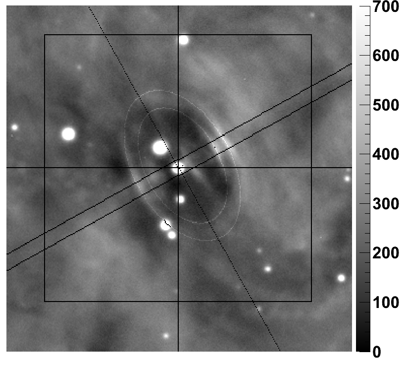
Figure 1: Optical image of the inner portion of the Crab nebula taken on 2011 April 13 and during a $\gamma$-ray flare (Buehler et al., 2012). North is up and east is to the left. The square covers a field of view of $50\>arcsec\times 50\>arcsec$ and is centred on the pulsar. The two parallel lines at a position angle of $-61^{\circ}$ measured east from north outline the region used to measure radial profiles. Two ellipses are shown that pass through the most prominent wisps at $8.0\>arcsec$ and $10.1\>arcsec$ NW of the pulsar. The aspect ratio of the ellipses (for all images) is 0.6 and their centre is offset from the pulsar by $0.8\>arcsec$ along a line (to the NW) that would connect the pulsar to the wisp peak emission. For display purposes we have removed low frequency variations in the image. The intensity units are arbitrary.

Table 1: Optical observation dates and seeing resolution

MJDa	Dateb	Seeingc
55518.1	2010/11/18	0.49
55532.0	2010/12/02	0.69
55557.9	2010/12/27	0.83
55564.1	2011/01/03	0.87
55570.0	2011/01/09	0.59
55598.8	2011/02/06	0.62
55612.9	2011/02/20	0.70
55647.9	2011/03/27	0.49
55664.9	2011/04/13	0.78
55810.2	2011/09/06	0.54
55863.2	2011/10/29	0.99
55881.1	2011/11/16	0.60
55922.1	2011/12/27	0.61
55954.9	2012/01/28	1.05
55986.9	2012/02/29	0.72
55998.9	2012/03/12	0.96
56013.9	2012/03/27	0.60
56025.9	2012/04/08	0.75
56033.9	2012/04/16	1.02
56140.2	2012/08/01	0.82
56141.2	2012/08/02	0.82
56153.2	2012/08/14	0.52
56159.2	2012/08/20	1.10
56176.2	2012/09/06	0.75

^a Modified Julian Date of start of observation.
^b UTC date.
^c Seeing FWHM in arcsec.

Optical data were obtained using the $2.56$m Nordic Optical Telescope (NOT) located in the Observatorio del Roque de los Muchachos on the Canary island La Palma. Altogether 24 images were taken from 2010 November until 2012 September using the Andalucia Faint Object Spectrograph and Camera (ALFOSC). The instrument employs a $2048\times 2048$ E2V chip with a gain of $0.327e^{-}$/ADU, a readout noise of $4.2e^{-}$ and a scale of $0.19\>arcsec\>pixel^{-1}$ giving a field of view of $6.5\times 6.5$ arcmin. Two to four exposures of $200-300$s were made through the I-band filter (NOT filter #12, $\lambda_{c}$ around $800$nm) at each epoch. The effective seeing resolution depends on observing conditions and ranges between $0.49\>arcsec$ and $1.1\>arcsec$. Table 1 lists the dates and seeing resolution for each optical observation. Fig. 1 shows one of the 24 optical images.

The images were processed first by subtracting the average bias image and then dividing by a twilight-sky flat-field image. The fringe pattern was removed using a fringe correction image created from archival NOT data taken using the same instrument configuration. After scaling and subtracting the fringe correction image, the fringe pattern was no longer visible. Individual frames were then registered using 8 stars in the vicinity of the pulsar and then averaged.

We checked the NOT pixel scale using a HST-legacy archive image of the Crab pulsar obtained with the Wide Field and Planetary Camera 2 (WFPC2) on 1995, August 14. Using the Planetary Camera portion of the image we selected two pairs of unsaturated stars within 25 arcsec of the pulsar and determined the distance between the two stars in each pair using the $0.05\>arcsec\>pixel^{-1}$ pixel scale of the image. Measuring the distances of the same pairs in the NOT image we arrived at NOT pixel scale of $0.1902$ and $0.1904\>arcsec\>pixel^{-1}$. Hence the adopted pixel scale $0.19\>\>arcsec\>pixel^{-1}$ is expected to be accurate to within 0.2%.

Sky background was subtracted from the average frames by fitting two models to the “pure sky” regions around Crab: a constant and a low-order polynomial. The two methods generally agreed to better than $1.2$% when extrapolated to the location of the pulsar. We use the constant in what follows. Flux calibration used the comparison star sequence given in Sandberg & Sollerman (2009). We used star 3 with I-band magnitude I = $16.26\pm 0.02$ from their calibration sequence to determine the zero point, $ZP$, by fitting a point spread function (PSF) model created from star 1 of Sandberg & Sollerman (2009) to star 3. The conversion from sky-subtracted counts, $N$ (ADU), to physical fluxes, $F$ ($\mu Jy$ per pixel), is then

$$F=2550*10^{-0.4(ZP-2.5\log N)}\ .$$ (1)

Since the calibration was obtained from a star in the Crab image, variations in atmospheric transparency are effectively accounted for and removed.

To check the accuracy of the calibration and background subtraction we studied the surface brightness of a relatively calm region close to the pulsar over our monitoring period. Using the 24 flux calibrated images we computed an average image and a sigma image, where in the latter each pixel value represents the rms flux variability at that pixel. Examining this image we identified a $2.8\>arcsec\times 2.8\>arcsec$ region $37\>arcsec$ South of the pulsar with a surface brightness close to that of the wisps (140 $\mu$Jy per $arcsec^{2}$) but with a small rms scatter compared to other regions near the pulsar. The rms scatter of the surface brightness from this region was 3.3%, somewhat larger than we would have expected due to inaccuracies in calibration and sky subtraction. Thus, some time variability of the Crab nebula may still be present, yet not at a level significant enough to alter our findings.

2.2 The X-ray Observations

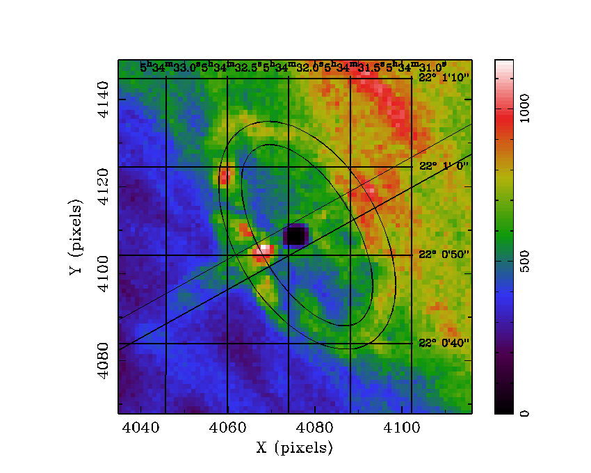
Figure 2: This Chandra X-ray image of the inner portion of the Crab nebula is the sum of the observations from the 2011 April, 14 to 28 during the $\gamma$-ray flare. The axes show RA and Dec (J2000) and ACIS detector pixels ($0.492\>arcsec\>pixel^{-1}$). The colour scale is in counts per ACIS pixel in the 0.5-8 keV band. The black feature with zero counts is the burned out image of the pulsar. The two parallel lines show the region from which the X-ray radial profiles were extracted and are the same as those in Fig. 1. The two ellipses show the region from which the azimuthal X-ray profile was extracted.

Subsequent to the discovery of $\gamma$-ray flaring in 2010 September (Tavani et al., 2011; Abdo et al., 2011) a series of Chandra X-ray Observatory observations was initiated on approximately a monthly cadence. Five Target of Opportunity observations were performed during the 2011 April $\gamma$-ray flare and the average of those 5 images is shown in Fig. 2. Chandra observations have continued, now as part of the Chandra general observer programme, yielding a sequence which covers approximately two years. As with our optical observations, the coverage is not continuous. Since Chandra is not allowed to point within $45\rm^{o}$ of the Sun, there is a 90 day interval during the summer when the Crab may not be observed. A list of the Chandra observations used for this paper is given in Table 2.

All data were taken with the back-illuminated Advanced CCD Imaging Spectrometer S3 (ACIS-S3) detector at the focus of the telescope in the energy band 0.5-8 keV. Owing to the Crab’s high flux, the observations were taken with the shortest possible frame time of $0.2$ s to minimize pileup. Even with this frame time, pileup impacts the brighter regions of the nebula. Telemetry saturation is also a issue with such a bright source, so we restricted data to a $300\times 300$ ACIS-pixel ($\approx 150\>arcsec\times 150\>arcsec$) region that covers the bright part of the nebula. The integration time was five ks for monitoring observations and 10 ks for the 5 observations following the 2011 April $\gamma$-ray flare. Due to telemetry saturation the effective exposure time was $600$ or $1200$ s (Table 2).

For the first three observations (Table 2) the dither amplitude of the spacecraft was set to zero. Since pileup characteristics may be different if the pulsar image is at the middle, edge or corner of a pixel, we then used a small ($1\>arcsec$ amplitude) dither for the remaining observations. This dither ensures that the pulsar and other sharp features in the nebula are averaged over a few pixels.

Level 2 event files were created using the CIAO tool acis_process_events using the EDSER option (Li et al., 2004) to improve the subpixel positioning. Due to severe pileup the pulsar does not appear in the image (Fig. 2). We did not simply rely on the Chandra aspect solution, but re-registered images making use of the readout trail (out-of-time image of the pulsar) to constrain one dimension and the burned out image of the pulsar to constrain the other coordinate.

Due to the different roll orientations of the observatory, the readout trail could introduce some bias in the azimuthal distribution. We removed this trail by computing the average number of counts per pixel due to the trail. Then, based on the actual number of counts seen in a pixel and our estimate of the number due to the readout streak, we randomly rejected events. Since this method is statistical, it is not perfect, but it will remove the principle brightness peak in the data due to the trail itself.

Table 2: Time-ordered list of Chandra observations with exposure time used for this paper.

ObsIDa	MJDb	Datec	Timed
13139	55467.2	2010/09/28	600
13146	55497.7	2010/10/28	600
13147	55528.5	2010/11/28	600
13204	55576.0	2011/01/15	600
13205	55608.7	2011/02/16	600
13206	55635.2	2011/03/15	600
13207	55663.6	2011/04/12	600
13150	55665.0	2011/04/14	1200
13151	55665.6	2011/04/14	1200
13152	55667.4	2011/04/16	1200
13153	55673.0	2011/04/22	1200
13154	55679.3	2011/04/28	1200
13208	55788.4	2011/08/15	600
13209	55819.2	2011/09/15	600
13210	55849.2	2011/10/15	600
13750	55892.7	2011/11/27	600
13751	55938.1	2012/01/12	600
13752	55967.4	2012/02/10	600
14416	56005.3	2012/03/19	600
13754	56039.1	2012/04/22	600
13755	56155.6	2012/08/16	600
13756	56181.9	2012/09/11	600

^a Chandra observation identifier.
^b Start of observation MJD.
^c UTC date.
^d Approximate effective exposure time in seconds.

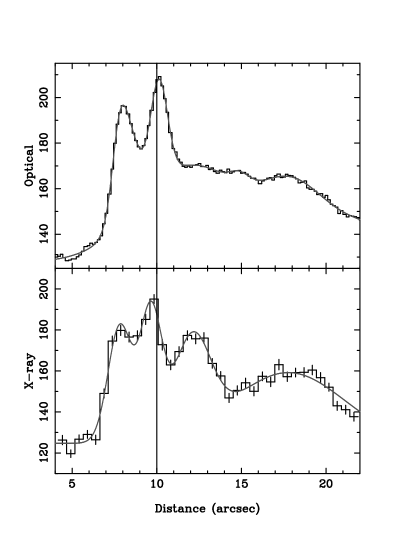
Figure 3: The upper panel shows the radial brightness distribution for the optical data for 2011 April 13 ($\mu Jy/arcsec^{2}$). The bottom panel shows the corresponding X-ray radial distribution for the average from 2011 April 14 until April 28 (counts per ACIS pixel). The solid lines denote a model fit based on a number of Gaussians. The vertical line at $10\>arcsec$ is drawn to emphasize that the optical and X-ray peaks do not exactly coincide.

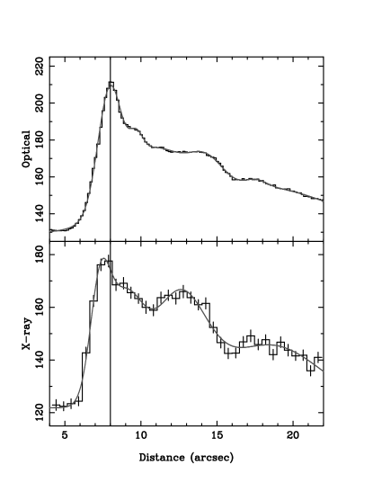
Figure 4: The upper panel shows the radial profile for the average of all the optical observations (in units of $\mu Jy/arcsec^{2}$). The lower panel shows the average radial profile for all the X-ray data (photon counts). The X-ray average does not include ObsIDs 13150 to 13154 to avoid biasing the average because of the concentrated coverage in 2011 April and to maintain a similar sampling cadence as for the optical data. The vertical line at $8\>arcsec$ shows that the brightest and closest optical and X-ray peaks do not exactly coincide.

3 Data analysis

Images were analysed to characterize the shape of the wisps in both the radial direction from the pulsar and angular extent about the pulsar. Our analysis to determine the radial distribution through the wisps restricted data to the narrow strip $3\>arcsec$ wide with position angle $-61\rm^{o}$ and is shown in Figs. 1 and 2. Optical and X-ray data were binned in radial bins of $0.11\>arcsec$ and $0.492\>arcsec$ respectively. The centre of the ellipse is assumed to be the same for all wisps. Significant differences ($<0.1\>arcsec$) cannot be detected within the resolution of individual optical or X-ray images. For azimuthal distributions we utilized $0.5\>arcsec$-wide elliptical annuli, on the sky and centred on the peak of the radial distribution.

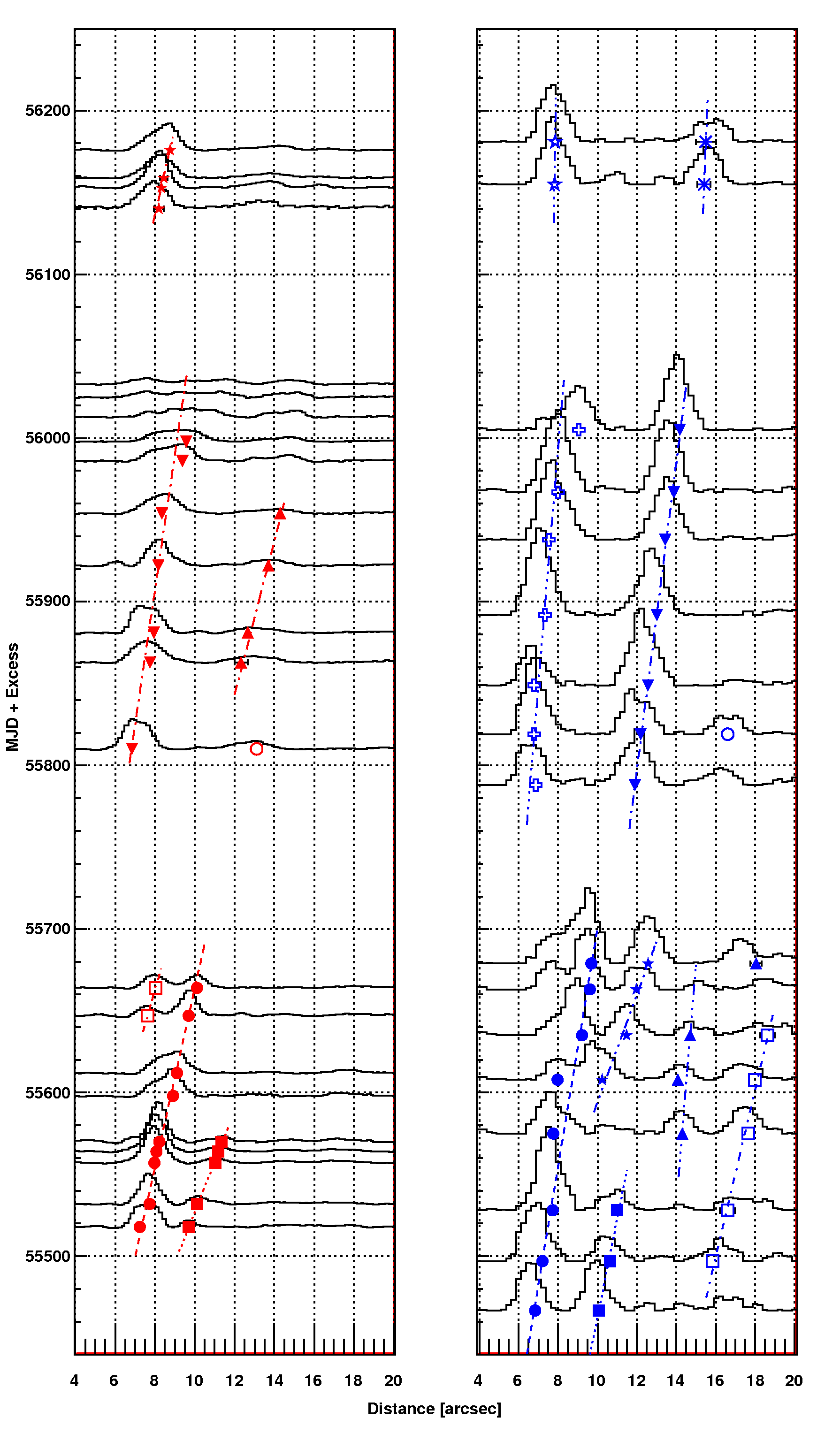
Figure 5: 23 optical and 17 X-ray radial profiles with low-frequency terms removed are plotted as a function of the distance NW of the pulsar. For clarity when one or more observations occur very close in time, we omit them from the figure. The omitted observations are optical - 56140.2 and X-ray - 55665.0, 55665.6, 55667.4, 55673.0 and 56039.1. For display purposes, low frequency terms have been removed using an algorithm from the ROOT-analysis package (Morháč et al., 1997). The symbols are placed on the distance axis to show the position of the peak of the Gaussian fitted to the original profile. So doing gives the illusion that the symbols are offset from the peak value. The lines, simply best guesses, are an interpretation of the time evolution of the position of a particular peak.

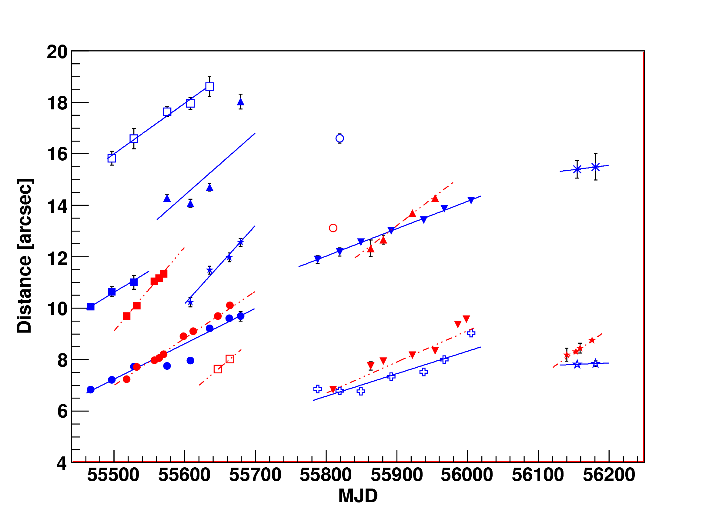
Figure 6: The radial positions of the wisp peaks as a function of time. Red and blue are used to indicate an optical or an X-ray wisp respectively. The symbols are the same as in Fig. 5.

Table 3: Velocities (in units of c) of the wisps identified in Figs. 5 and  6.

symbol	$arcsec/:d^{-1}$	(v/c)a	(v/c)b
Optical (red)
circle	0.018	0.21	0.29
box solid	0.033	0.38	0.44
triangle up	0.021	0.24	0.32
triangle down	0.012	0.14	0.21
star	0.019	0.22	0.30
X-rays (blue)
circle	0.014	0.16	0.24
box solid	0.017	0.19	0.28
box open	0.020	0.23	0.31
star solid	0.031	0.35	0.42
triangle up	0.024	0.28	0.36
triangle down	0.011	0.12	0.19
cross	0.009	0.10	0.16

^a Apparent velocity on the sky.
^b Deprojected velocity.

3.1 Analysis of the radial profile of the wisps

Throughout this paper we refer to “radial profiles”. This profile is simply the intensity distribution, within the parallel lines in Figs. 1 and 2 measured outwards from the pulsar towards the NW. We fit a constant plus a number of Gaussians to both optical and X-ray radial profiles. Initially a Gaussian is located at each peak seen in the profile. The model was then fitted using a least squares fitting method that allowed all parameters to vary. After the fit had converged, we then visually inspected to ensure that the main peaks had been properly located and if not the model would be modified, either by adjusting parameter values or adding an additional Gaussian, and then refitted.

An example of an optical and an X-ray radial profile measured close in time is shown Fig. 3. We see two prominent peaks in the optical and the presence of at least three peaks in the X-ray profile. In general, the peak closest to the pulsar is most usually identified with the location of the termination shock. Fig. 3 demonstrates that the X-ray peak at $10\>arcsec$ is located at a slightly different (and smaller) distance than the peak in the optical. The exposures in optical and X-rays in the figure are not precisely simultaneous and the average time difference is about 8 d. However, even if we account for the apparent radial motion (§ 3.2), the X-ray wisp is still closer to the pulsar than the nearest optical wisp.

Fig. 4 top plots the radial profile of the average of all the optical observations. Notice the strong peak at $8\>arcsec$ showing that the optical wisps are brightest at this distance from the pulsar and then fade at larger distances. Fig. 4 bottom shows the same plot in X-rays averaged with the same sampling interval as for the optical. The innermost X-ray arc, at $\sim 7.5~{}arcsec$, is brightest, and closer to the pulsar than in the optical. Similarly, the further from the pulsar, the fainter the average intensity in the radial profile.

3.2 The radial evolution of the wisps as a function of time

Fig. 5 is a graphical representation showing most of the optical and X-ray radial projections as a function of the angular distance from the pulsar. For display purposes only, low frequency terms have been subtracted. The algorithm applied was the TSpectrum background subtraction algorithm from the ROOT-package (Morháč et al., 1997).

In Fig. 5 we also trace the outward motion of a particular peak by drawing a line through the position of what appears to be the same peak but at different times. There appears to be possibly five distinct progressions of peaks in the optical data and possibly seven in X-rays. We have not attempted to connect progressions across summer gaps, but one could do so. As the slopes of the lines indicating the outward progression are different, so are the inferred velocities. These are given in Table 3 where we list the measured quantity i.e. the apparent velocity on the sky in $arcsec/day$, and, assuming a distance of 2 kpc, the deprojected physical velocity. For deprojection we use an inclination angle of $57^{{}^{\circ}}$ (Weisskopf et al. (2012) and references therein). Fig. 6 also compares the motion of the peaks in the radial profiles as a function of time. The figure indicates that most of the time an X-ray wisp appears close to the pulsar, so does an optical wisp that is slightly further away from the pulsar.

Fig. 7 presents a different yet equally interesting, picture and comparison of the evolution of the peak fluxes in the azimuthal distributions as a function of time. To construct this figure we used a time spacing of 10 d. If an observation took place at any time within the 10 d interval the data were included as a column in the figure. For short gaps in the time sequence, we performed a linear average of the closest columns that contain data. Thus, if there was a two column gap, we would add two thirds of the previous observation to one third of the following observation to fill in the first missing column. For the second missing column, the weights were reversed. If the wisps in two data sets overlap, this method will cause the wisp to appear to move from the location in the first data set to the location seen in the second across the gap. If the features do not overlap, then features in the first data set will appear to fade as new features appear to grow. We have determined that the gap in the summer break is too long for our interpolation method to work and thus it is empty.

All the features seen in Fig. 5 can also be seen pictorially in Fig. 7. Note that the width of neighbouring peaks in the X-ray and optical do not appear to be correlated. In the X-ray portion of Fig. 7 we also see the slow outward motion of the outer boundary where the colour changes from green to blue. This boundary is close to $20\>arcsec$ from the pulsar for the earliest observations, yet moves to near $25\>arcsec$ by the end of the sequence. This outward motion of the boundary roughly matches the apparent outward motion of the brighter wisps. Although the bright wisps can be seen in both the X-ray and the optical,some X-ray peaks do not appear to have a nearby optical companion. Furthermore, the positions of the optical wisps do not precisely align with the positions of the X-ray wisps. That would seem to imply that the individual evolution of optical and X-ray wisps is different, but, becuse of their proximity they are related. Fig. 7 also makes it clear that new wisps form in the inner region roughly once per year.

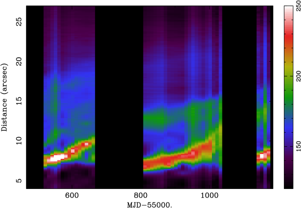
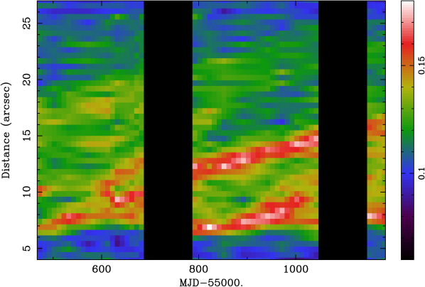
Figure 7: The two panels compare the radial evolution of the optical (upper panel) and X-ray (lower panel) wisps. For clarity, data were interpolated between observations but not across the large gaps imposed by sun constraints. The unit for the colour scale is $\mu J/arcsec^{2}$ for the upper panel and counts for the lower panel.

Figure 8: The azimuthal distributions of two optical wisps observed on 2011 April 13 at distances of $8.0\>arcsec$ and $10.1\>arcsec$ from the pulsar. The angle is the azimuthal angle of the deprojected ellipse. $0^{\circ}$ was set by the peak of the distribution.

3.3 Analysis of the azimuthal profile of the wisps

Good statistics for the optical data allow us to measure the azimuthal intensity profile for each observation. These analyses measure the azimuthal intensity distribution of the flux in the ellipse-like shapes to the NW of the pulsar. Elliptical shapes arise presumably because they are formed in a circular ring more or less in the equatorial plane of the pulsar. In X-rays one finds that the aspect ratio of the innermost ellipse (the location of the presumed termination shock) is 0.49 and the pulsar is displaced along the axis of symmetry by $\approx 0.9\>arcsec$ below the plane of the ring and along the minor axis which is at a position angle of $-60\rm^{o}$ (Weisskopf et al., 2012). It is more difficult to determine these parameters in the visible primarily because a complete ring is not observed. Nevertheless, as may be seen in Fig. 1, assuming an elliptical shape with the offset and aspect ratio as specified follows the path of the optical data extremely well. Since we have already found that the wisps in both bands typically do not line up, there is no reason to expect that the ellipses be identical.

Fig. 8 shows the azimuthal distribution of the intensity for two of the optical wisps at distances of $8.0\>arcsec$and $10.1\>arcsec$ from the pulsar. The distributions shown in the figure were based on a $0.5\>arcsec$-wide elliptical annulus with $0.6$ aspect ratio.

The X-ray data are noisier than the optical data so we considered both the average of the 2011 April data and the average of all except for the 2011 April data. Within errors, the width of these two distributions were identical. The azimuthal variation was obtained from an elliptical annulus $0.5\>arcsec$ wide and $8.0\>arcsec$ from the pulsar as shown in Fig. 2.

Comparing the X-ray angular distribution with the optical one, it is important to note that the latter has a sharper peak than that seen in X-rays. The full width at half-maximum (FWHM) of the distribution in optical is around $30^{\circ}$ while the X-ray distribution has an FWHM of around $70^{\circ}$.

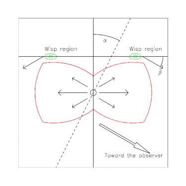
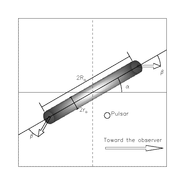
Figure 9: Left-hand panel: Schematic structure of the termination shock (red) cross-section. The pulsar, from which a relativistic radial wind originates, is located at the central circle and the solid vertical line represents the axis of symmetry of the nebula. The large arrow indicates the direction towards the observer, while the dashed line represents the plane of the sky. The wind slows down and is diverted in a termination shock which has an oblique shape due to wind anisotropy. Wisps can form anywhere along the termination shock. A wisp (solid green circle) will appear bright within the wisp region (solid green ellipse) when the particle motion is directed towards the observer. The wisp will fade as it moves out from this region. The symbol $\alpha$ is the angle between the nebular axis and the plane of the sky and $\beta$ is the angle between the plane of the wisps and the flow direction in the wisp regions. Right-hand panel: Schematic of a single wisp modelled as an emitting ring. The dashed line represents the plane of the sky and $R_{o}$ and $r_{o}$ are the major and minor radii of the torus respectively.

4 Model fitting and theoretical discussion

The magnetohydrodynamic (MHD) model developed with success in the past years (Komissarov & Lyubarsky, 2003, 2004; Del Zanna et al., 2004; Bucciantini et al., 2005; Del Zanna et al., 2006; Volpi et al., 2008; Camus et al., 2009) explains the existence of rings and wisps observed in pulsar wind nebulae (PWNe) in terms of axisymmetric enhancements of the emissivity immediately downstream of the termination shock. Due to the anisotropy of the pulsar wind luminosity, and the related oblate shape of the termination shock (Del Zanna et al., 2004), axisymmetric regions form inside the nebula where the emissivity towards the observer is higher, either because of local compression of the magnetic field, or because of Doppler boosting. In general it is found that typical flow speeds immediately downstream of the termination shock can be as high as $0.7$c, and the emission is dominated by Doppler boosting.

Komissarov & Lyubarsky (2004) have shown that both the wisps and the knot observed in the Crab nebula can be qualitatively explained by the geometry of the flow (Fig. 9). In particular the association of the wisps with the wind termination shock is due to the fact that they originate in the flow immediately downstream of the shock itself. A simplified model for a wisp can be built on the assumption that a wisp is due to a torus- or ring-like region within the nebula. This region can appear bright or dim depending on Doppler boosting due to the relative direction of the observer, and the particle flow. This boosted-ring model appears in alternative explanations for the origin of the wisps, e.g. in term of ion-cyclotron compression (Spitkovsky & Arons, 2004) or cooling instabilities (Foy & Hester, 2009). The boosting is required in all of these models to explain the azimuthal luminosity profile of the wisps, and the fact that one side of the nebula (the front side) is brighter than the back side. This idea has been adopted in the past (Romani & Ng, 2003; Ng & Romani, 2004; Romani et al., 2005) to model the jet torus structure observed in X-rays in several PWNe, and to estimate typical flow speeds in these systems.

MJD	Dist	$V_{fl}$	$U_{fl}$	$V_{fl,min}$	$V_{fl,max}$	$r_{o}/R_{o}$
55518	5.0	0.87	1.76	0.80	0.92	0.01
55518	7.2	0.96	3.68	0.96	0.97	0.01
55518	8.0	0.95	2.89	0.93	0.96	0.01
55518	9.7	0.80	1.33	0.75	0.85	0.01
55532	7.7	0.94	2.76	0.93	0.95	0.01
55532	10.1	0.83	1.49	0.75	0.87	0.01
55557	8.0	0.94	2.76	0.93	0.95	0.01
55557	10.9	0.90	2.06	0.84	0.93	0.04
55564	8.1	0.95	3.04	0.93	0.96	0.01
55564	11.2	0.92	2.35	0.88	0.96	0.04
55570	8.2	0.95	3.04	0.94	0.96	0.01
55570	11.4	0.92	2.35	0.87	0.94	0.03
55598	8.9	0.94	2.76	0.92	0.95	0.04
55598	11.1	0.90	2.06	0.85	0.92	0.03
55598	12.7	0.70	0.98	0.60	0.85	0.04
55612	8.4	0.93	2.53	0.90	0.95	0.03
55612	9.1	0.93	2.53	0.90	0.94	0.01
55612	11.4	0.80	1.33	0.70	0.87	0.02
55647	7.6	0.97	3.99	0.95	0.98	0.01
55647	9.7	0.97	3.99	0.96	0.98	0.01
55647	12.4	0.90	2.06	0.93	0.85	0.01
55664	5.8	0.85	1.61	0.77	0.91	0.04
55664	8.0	0.93	2.53	0.91	0.95	0.04
55664	10.1	0.91	2.19	0.87	0.93	0.04
55810	6.9	0.93	2.53	0.90	0.95	0.07
55810	12.5	0.93	2.53	0.89	0.96	0.06
55863	5.0	0.80	1.33	0.73	0.90	0.02
55863	7.6	0.93	2.53	0.90	0.95	0.07
55863	12.5	0.93	2.53	0.90	0.95	0.06
55881	7.2	0.95	3.04	0.94	0.96	0.01
55881	8.0	0.94	2.75	0.93	0.95	0.01
55881	10.2	0.80	1.33	0.70	0.87	0.04
55881	12.6	0.90	2.06	0.85	0.93	0.06
55922	6.0	0.86	1.68	0.82	0.90	0.02
55922	8.2	0.93	2.53	0.90	0.97	0.04
55954	8.6	0.90	2.06	0.89	0.93	0.07
55954	12.5	0.90	2.06	0.85	0.95	0.07
55998	9.6	0.92	2.35	0.89	0.95	0.10
56013	7.6	0.93	2.53	0.90	0.95	0.03
56013	8.9	0.92	2.35	0.89	0.94	0.03
56025	7.5	0.94	2.75	0.92	0.97	0.04
56025	9.3	0.90	2.06	0.86	0.92	0.03
56033	7.6	0.94	2.75	0.92	0.97	0.04
56033	9.6	0.87	1.76	0.85	0.89	0.04
56140	8.0	0.95	3.04	0.93	0.96	0.05
56140	13.6	0.85	1.61	0.80	0.88	0.10
56141	8.0	0.95	3.04	0.93	0.96	0.05
56141	13.8	0.80	1.33	0.70	0.85	0.10
56153	8.3	0.96	3.43	0.94	0.97	0.02
56159	8.3	0.95	3.04	0.93	0.96	0.06
56176	8.6	0.95	3.04	0.93	0.96	0.06

Table 4: Fitted parameters for the optical wisps. The table lists the MJD, the distance to the pulsar, the flow velocity in units of c, the boosting four-velocity, and the minimum and maximum flow velocities still compatible with the fit and the thickness of the torus. In all cases we found $\alpha=\beta=37^{\circ}\pm 4^{\circ}$.

With reference to Fig. 9, a wisp originates from a region shaped like a torus, with major radius $R_{o}$ and a minor radius $r_{o}$. The ratio $r_{o}/R_{o}$ we call the thickness of the torus. The plane of the torus has an inclination $\alpha$ with respect to the line of sight, which, within the axisymmetric approximation, is equal to the angle between the nebular axis and the plane of the sky. The fluid in the torus has a uniform flow speed $V_{fl}$, confined in meridianal planes (planes containing the nebular axis). The azimuthal component of this flow speed is assumed to be $0$. $V_{fl}$ forms an angle $\beta$ with respect to the plane of the torus.

We want to stress here that $V_{fl}$ is the flow speed of particles in the wisp, and should not be confused with the observed wisp velocity, which we have discussed previously. The two are not the same simply because the wisp velocity traces the propagation of the ring in the nebula as a wave, and not the bulk motion of particles. For simplicity we assume uniform synchrotron emissivity inside the torus. In this picture the torus contains a fully ordered toroidal magnetic field, but models can also be built with a chaotic magnetic field (see below for a discussion). The emissivity towards the observer is computed as in previous works (Komissarov & Lyubarsky, 2003, 2004; Del Zanna et al., 2004; Bucciantini et al., 2005; Del Zanna et al., 2006; Volpi et al., 2008; Camus et al., 2009) and a synchrotron map is built integrating the contribution of the various parts of the torus along the line of sight. The emitting particles are assumed to be distributed as a power-law in energy with an index $-2.35$ in agreement with values estimated from optical observations and spectral modelling of the Crab nebula (Bucciantini et al., 2011). This also applies for the X-ray wisp(s). In the MHD model of PWNe, the wisps are assumed to be located immediately downstream of the termination shock, where particles are accelerated and magnetic field is compressed. Given that the wisps originate from the termination shock, synchrotron cooling should be negligible and the particle distribution unaffected.

The wisps appear brighter to the NW of the pulsar and almost fade to the sky background level in the southeast mostly due to Doppler boosting, given that the flow velocity is generally directed towards the observer in the NW, while in the southeast it points away. We want to stress here that the plane of the torus does not necessarily need to coincide (even if it is parallel) with the equatorial plane of the pulsar, but there can be an offset between the two. Such an offset, however, has no consequences in the model for the wisp emissivity.

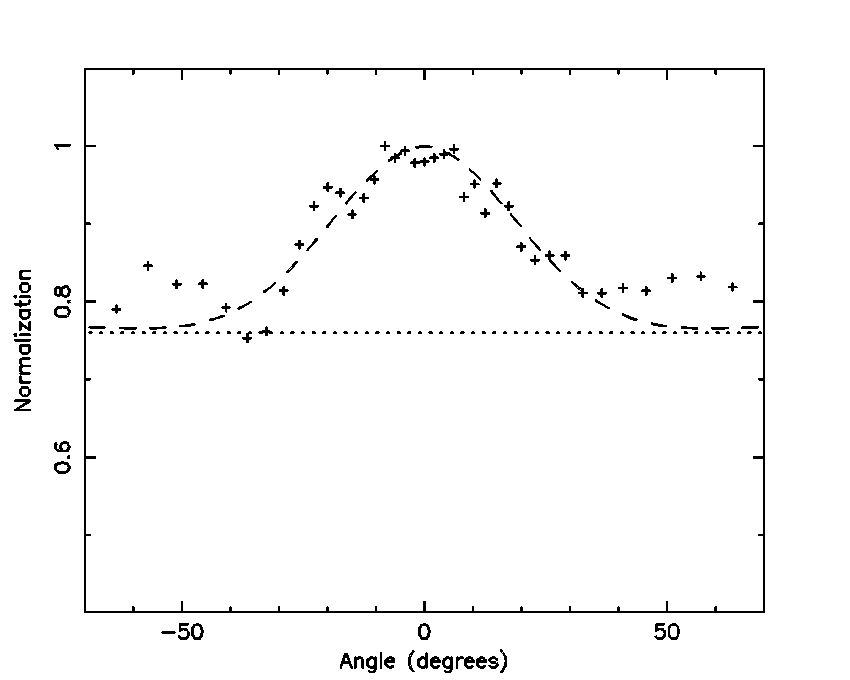
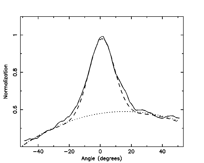
Figure 10: Left-hand panel: The average azimuthal X-ray intensity distribution (normalized to its maximum) in an elliptical annulus at a distance of $8\>arcsec$ to the NW of the pulsar. The dashed line shows a simulated azimuthal distribution as discussed in §4. The dotted line denotes a“background” level based on a simple 2D polynomial model for the local azimuthal intensity. The dashed line shows a simulated azimuthal distribution as discussed in §4. Right-hand panel: Same as the left-hand panel but for the average optical wisp centred at a distance of $8arcsec$ from the pulsar.

We fit the optical data to this model as follows:

• We select a set of input parameters $r_{o}/R_{o}$, $\alpha$, $\beta$, and $V_{fl}$.

• An emission map is built (the emission is normalized to the maximum).

• The emission map is convolved with the PSF of the observation.

• Emission profiles are extracted both along the wisp and along the axis of the nebula.

• The simulated radial and azimuthal profiles are added to an assumed background and then compared with the data. The background is based on a simple 2D polynomial least-squares fit, as shown in Fig. 10 and Fig. 11. Note that we found no significant difference in the results if fits were performed to the background subtracted data. Furthermore, there were no significant differences in the boosting speed if the background in the wisp region is assumed to be uniform, or to have low frequency components.

• This procedure is repeated until a set of input parameters are found that provide a reasonable fit. The best-fitting parameters are obtained by minimizing the residuals in the brightest part of the wisp, where the background subtracted intensity is $>50$% of its maximum value.

The results for the optical wisps are presented in Table 4. We can also roughly quantify the uncertainty in the various parameters. The upper (lower) limit on the flow boosting velocity $V_{fl}$ given in Table 4, corresponds to a model which gives a wisp whose FWHM is 15% narrower (larger) than the observed value. Fig.  11 compares one of the optical observations and the result from a simulated map, using the best-fitting input parameters from Table 4.

We stress here that our procedure does not take into account time-of-flight delays. However, given that the extent of the optical wisps is usually within $\pm 20^{\circ}$ from the axis, this effect should be negligible.

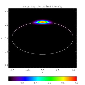
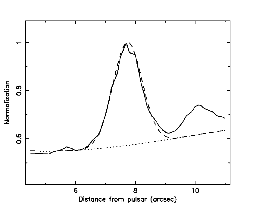
Figure 11: Upper panel: Simulated synchrotron map of the optical wisp for MJD=55532 and at a distance of $7.7\>arcsec$ derived using the fitted parameters in Table 4. The axes are in arbitrary units normalized to the wisp major radius $R_{o}$. Colours indicate the level of the flux, normalized to the maximum. Middle panel: the solid line is the optical profile of the wisp along the nebular axis, while the dashed line is obtained from the simulated synchrotron map. The dotted line represents the (assumed) background. Lower panel: Same as the middle panel but for the azimuthal profile.

There are several interesting points to note:

• Typical flow speeds inferred from our model range between $V_{fl}=0.8$c and $V_{fl}=0.95$c. Using a chaotic magnetic field distribution leads to even higher velocities.

• The angle $\beta$ is almost equal to the angle $\alpha$.

• The wisps appear to be unresolved and the ratio $r_{o}/R_{o}$ is less than $0.1$.

The high values of the flow speed correspond to boosting factors that are in excess of typical values found in MHD simulations by about a factor of between 2 and 5 depending on which value of $\beta$ one chooses. This is related to the narrow extent of the optical wisps which fade to the sky background level within $\pm 20^{\circ}$ from the axis. This is also connected to the fact that $\beta\approx\alpha$, implying that the flow speed on the front side of the nebula is directed towards the observer. If $\beta$ differs from $\alpha$ by more than $3^{\circ}-5^{\circ}$, it is not possible to reproduce the azimuthal wisp luminosity, independently of $V_{fl}$. The minimum value of $V_{fl}$ is obtained for $\beta=\alpha$. Moreover, it appears that the optical wisps are consistent with narrow features, possibly close to emitting sheets. It is also interesting to note that there is a trend in the observed flow speeds as a function of wisp location, with higher values for inner wisps, as shown in Fig. 12.

A comparison between the azimuthal profile in optical and X-rays has also been done. However, for the X-ray data, in order to have sufficient statistics, instead of a single epoch, we consider first an average over the entire set of observations and only for the inner (brighter) X-ray wisp region located $\sim 8\>arcsec$ away from the pulsar (Fig.  10). We also repeated this analysis averaging just the 2011 April data with similar results.

To eliminate the possibility that the difference was due to averaging the X-ray data, we averaged the optical data over all of our epochs. Results were shown in Fig. 10. The resulting model parameters are $r_{o}/R_{o}=0.1$, $\alpha=\beta=35^{\circ}$ for both optical and X-ray, while $V_{fl}=0.6c\pm 0.1c$ for the X-ray and $V_{fl}=0.91c\pm 0.03c$ for the optical. We may associate this with a boosting four-velocity $U_{fl}=(V_{fl}/c)/\sqrt{[1-(V_{fl}/c)^{2}]}$ of 0.75 for X-ray and 2.20 for optical (i.e. a factor of 3.13). Thus, we can safely conclude that the azimuthal extent of this X-ray wisp is larger than in the optical and, within the context of our model, this implies lower inferred speeds for the particles producing the X-rays. The fitted parameters for the optical wisps, however, raise the question if the boosted ring model is in fact appropriate. The MHD model has been developed mostly to reproduce Chandra observations but it is also evident from our study that X-ray and optical wisps are not produced by the same particle distribution: they do not coincide in location or in terms of the degree of Doppler boosting. It is not our intention here to develop and provide an alternative explanation for the azimuthal luminosity of the optical wisps, but we can point to a few possible solutions.

• Optical wisps appear to originate in the transition layer at the termination shock itself. This is consistent with the thin-sheet hypothesis and the idea that, at the shock itself, the flow speed is higher than in the downstream region. It remains to be proven that the geometry of the shock can allow for such configurations.

• Emissivity is enhanced along the axis of the nebula because of local clumpiness. Clumps are observed in X-rays, called by some sprites, and they have a more or less stable location. However, why in optical, these clumps should be located along the axis of the nebula is not clear.

• If the particle distribution in a wisp is non-isotropic, then the emissivity has a stronger dependence on the inclination of the magnetic field with respect to the line of sight than in the isotropic case. It is not clear, however, what the degree of anisotropy needs to be and if it can be produced by known acceleration mechanisms.

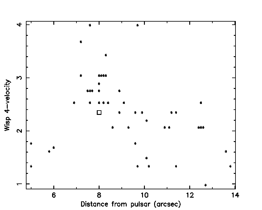
Figure 12: Boosting four-velocity $(V_{fl}/c)/\sqrt{[1-(V_{fl}/c)^{2}]}$ for the optical wisps as a function of their distance from the pulsar. The square denotes the boosting four-velocity obtained from the averaged optical profile. Note that the data points at radii $\leq 7\>arcsec$ are most likely not due to wisps, but other optical features such as the halo (Hester, 2008), in which case the model would not apply.

5 Conclusion

We find that approximately once per year optical and X-ray wisps appear and peel off from the region commonly associated with the termination shock of the pulsar wind. Although the X-ray and optical wisps are related by their proximity and their outward motion, they are not precisely aligned. It is also interesting to note that the optical and radio wisps are separated from each other (Bietenholz et al., 2004).

Interestingly, the time interval between $\gamma$-ray flares is also about 1 y leading to the speculation that the flaring may somehow be associated with wisp formation. However, since a new wisp did not form in coincidence with the $\gamma$-ray flare of 2011 April which took place during this study, the speculation requires a theory that has the formation of the wisps either substantially ($\approx$month) preceding a $\gamma$-ray flare, or being an unrelated phenomenon.

The wisps propagate outward with velocities projected on to the sky ranging from $0.1$(v/c) to $0.4$(v/c) (Table 3). If anything, there appears to be a trend for the projected velocity of a wisp increasing, the further it is from the pulsar, perhaps implying a re-acceleration pmechanism for the wisp itself. More likely, this apparent behaviour may be a result of the more complicated three-dimensional geometry and there may be no need for such re-acceleration when properly deprojected. A word of caution is that one might be confusing features in the counter-jet with structure in the wisps.

Within the context of an MHD modelling, we find that optical wisps are more strongly Doppler-boosted than the X-ray wisps. In particular, we found that the azimuthal luminosity profile of the X-ray wisps is fully compatible with typical boosting factors found in MHD simulations of PWNe. Instead, the azimuthal luminosity profile of the optical wisps requires particles velocities that are incompatible with the results of global numerical modelling of PWNe (Komissarov & Lyubarsky, 2003; Bucciantini et al., 2005). This should be investigated with future modeling.

References

- Abdo et al. (2011) Abdo A. A. et al. 2011, Science, 331, 739
- Bietenholz et al. (2004) Bietenholz M. F., Hester J. J., Frail D. A., Bartel N., 2004, ApJ, 615, 794
- Bucciantini et al. (2011) Bucciantini N., Arons J., Amato E., 2011, MNRAS, 410, 381
- Bucciantini et al. (2005) Bucciantini N., del Zanna L., Amato E., Volpi D., 2005, A&A, 443, 519
- Buehler et al. (2012) Buehler R., et. al., 2012, ApJ, 749, 8
- Camus et al. (2009) Camus N. F., Komissarov S. S., Bucciantini N., Hughes P. A., 2009, MNRAS, 400, 1241
- Del Zanna et al. (2004) Del Zanna L., Amato E., Bucciantini N., 2004, A&A, 421, 1063
- Del Zanna et al. (2006) Del Zanna L., Volpi D., Amato E., Bucciantini N., 2006, A&A, 453, 621
- Foy & Hester (2009) Foy J. P., Hester J., 2009, Abs. 213, BAAS, 41, p. 488.01
- Hester (2008) Hester J. J., 2008, ARA&A, 46, 127
- Hester et al. (2002) Hester J. J. et al., 2002, ApJ, 577, L49
- Hester et al. (1995) Hester J. J. et al. 1995, ApJ, 448, 240