A fast direct solver for quasi-periodic scattering problems

Abstract.

We consider the numerical solution of the scattering of time-harmonic plane waves from an infinite periodic array of reflection or transmission obstacles in a homogeneous background medium, in two dimensions. Boundary integral formulations are ideal since they reduce the problem to $N$ unknowns on the obstacle boundary. However, for complex geometries and/or higher frequencies the resulting dense linear system becomes large, ruling out dense direct methods, and often ill-conditioned (despite being 2nd-kind), rendering fast multipole-based iterative schemes also inefficient. We present an integral equation based solver with $O(N)$ complexity, which handles such ill-conditioning, using recent advances in “fast” direct linear algebra to invert hierarchically the isolated obstacle matrix. This is combined with a recent periodizing scheme that is robust for all incident angles, including Wood’s anomalies, based upon the free space Green’s function kernel. The resulting solver is extremely efficient when multiple incident angles are needed, as occurs in many applications. Our numerical tests include a complicated obstacle several wavelengths in size, with $N=10^{5}$ and solution error of $10^{-10}$, where the solver is 66 times faster per incident angle than a fast multipole based iterative solution, and 600 times faster when incident angles are chosen to share Bloch phases.

1. Introduction

Numerical modeling of the scattering of linear time-harmonic waves from materials with periodic geometry plays a key role in modern optics, acoustics, signal processing, and antenna design. Periodic diffraction problems where numerical modeling is crucial include the design of gratings for high-power lasers [6], thin-film solar cells [4] and absorbers [39], process control in semiconductor lithography [34], linear water-wave scattering from pillars [37], and radar sensing of ocean waves. In all such problems, an incident plane wave generates a scattered wave which (in the far field) takes the form of a finite sum of plane waves at known Bragg angles, whose amplitudes are desired.

Several challenges arise in the efficient numerical solution of grating scattering problems: (i) the period of the gratings can be many wavelengths in size, (ii) in many applications (such as photovoltaic [4] or solar absorber design [39]) solutions are needed at many incident angles and/or frequencies, (iii) the scatterer may have physical resonances in the form of guided modes (see Remark 2.1), which leads to ill-conditioned problems, and (iv) so-called Wood’s anomalies may occur, that is, scattering parameters (incident angle and frequency) for which one of the Bragg angles lies precisely along the grating. Note that challenges (iii) and (iv) are distinct: (iii) is a physical resonance leading to an ill-posed problem (see the reviews [41, 30]), whereas Wood’s anomalies do not cause ill-posedness—and yet they do cause problems for many numerical schemes.

In most problems of interest, gratings consist of homogeneous media delineated by sharp interfaces; hence the corresponding partial differential equations (PDEs) have piecewise-constant coefficients. This manuscript focuses on the following two-dimensional Dirichlet boundary value problem, which models acoustics with sound-soft obstacles, or electromagnetic scattering in TM (transverse magnetic) polarization from perfect electric conductors (where $u$ represents the out-of-plane electric field [5]). We seek the scattered wave $u$ which solves,

(1.1) $$\begin{split}(\Delta+\omega^{2})u(\textbf{x})&=0\ \ \qquad\qquad\qquad\textbf{x}:=(x,y)\in\mathbb{R}^{2}\setminus\overline{\Omega_{\mathbb{Z}}}\\ u(\textbf{x})&=-u^{\rm i}(\textbf{x})\qquad\qquad\textbf{x}\in\partial\Omega_{\mathbb{Z}}\\ u&\quad\mbox{radiative as }\ \ y\to\pm\infty~{},\end{split}$$

where $\Omega\subset\mathbb{R}^{2}$ is a single bounded obstacle which is repeated to form an infinite grating of obstacles (denoted by $\Omega_{\mathbb{Z}}$) of period $d$ along the $x$-axis (see Fig. 1.1(a)). A plane wave with frequency $\omega$, angle $\theta\in(-\pi,0)$, and wavevector $\textbf{k}=(\kappa^{\mbox{\tiny i}},k^{\mbox{\tiny i}})=(\omega\cos\theta,\omega\sin\theta)$ is incident; hence $u^{\rm i}(\textbf{x})=e^{i\textbf{k}\cdot\textbf{x}}$ outside the obstacles and vanishes inside. It is easy to see from (1.1) that the total field $u^{t}=u^{\rm i}+u$ vanishes on ${\partial\Omega}$: this is the physical boundary condition. For the exact radiation condition on the scattered field $u$ see (2.5)-(2.6). The incident field, and hence the scattered field, satisfy a quasi-periodicity condition,

(1.2) $$u(x+d,y)=\alpha u(x,y)\qquad\forall(x,y)\in\mathbb{R}^{2}~{},$$

where $\alpha:=e^{i\kappa^{\mbox{\tiny i}}d}=e^{i\omega d\cos\theta}$ is known as the Bloch phase. We will also consider the transmission problem corresponding to dielectric obstacles (see section 5).

Integral equation formulations are a natural choice for problems with piecewise-constant coefficients such as (1.1): they exploit this fact by reducing the problem to an integral equation whose discretization involves $N$ unknowns living on the boundary alone. This has many advantages over finite elements or finite difference schemes: it reduces the dimensionality by one, allowing for more complicated boundaries to be solved to high accuracy with a small $N$, and is amenable to easily implemented high-order quadratures.

In the grating application, the infinite boundary $\partial\Omega_{\mathbb{Z}}$ must be reduced to the boundary of a single obstacle ${\partial\Omega}$; there are two main approaches to this task of “periodizing” the integral equations.

The first approach replaces the Green’s function (fundamental solution) that appears in the kernel of in the integral operators by its quasi-periodized version [30] (which satisfies (1.2)). This is used in two dimensions by Bruno–Haslam [10] and in three by Nicholas [36] and Arens [2]. However, this fails as parameters approach a Wood’s anomaly, because the Green’s function does not exist there. One cure (in the case of a connected interface) is to use the quasi-periodic impedance half-space Green’s function [32, 3]. However, all such periodized kernel methods do not scale well to large $N$ because dense matrices must be filled at a cost of order a millisecond per element [26].

The second approach, which is robust at all parameters including at or near Wood’s anomalies, is to return to the free-space Green’s function and instead periodize using a small number of additional unknowns on artificial unit-cell walls. The condition (1.2) is then imposed directly in the linear system. This is used by Wu–Lu [43], and also by one of the authors in [5]. Further advantages of the second approach include: the low-rank nature of the periodizing is explicit (no dense matrices of periodized Green’s evaluations are needed), and that free-space boundary integral equation quadratures and codes may be used without modification.

In this paper, we present a fast direct solver for the formulation in [5], that can handle, in reasonable computation times, complicated boundaries that both demand large $N$ and cause ill-conditioning. Section 2 reviews the derivation of the periodized integral formulation in the Dirichlet setting (1.1).

Like many boundary integral equations for two-dimensional domains, this gives a linear system that could be solved via an iterative solver (e.g. GMRES) coupled with a fast matrix-vector multiplication scheme such as the fast multipole method (FMM) [12]. Unfortunately, when the system is ill-conditioned (which often occurs for complicated geometry) it can take hundreds of iterations for such an iterative solver to converge, or worse, it may never converge to an acceptable accuracy. Additionally, iterative methods are not able to efficiently solve problems with multiple right hand sides that occur when the response is needed at multiple incident angles. This has motivated in recent years the development of a collection of fast direct solvers. These solvers utilize internal structure (essentially low-rank off-diagonal blocks) to construct rapidly an approximate inverse of the dense matrices resulting from the the discretization of integral equations. For many problems, the computational cost is $O(N\log^{k}N)$ with typically $k=0,1,$ or $2$ [22, 9, 31, 7, 33, 42], which can be orders of magnitude smaller than traditional $O(N^{3})$ dense direct methods.

In addition to being fast, the solvers are robust and construct the approximate inverse in such a way that it can be applied in with $O(N)$ (with small constant) computational cost. In this work, we choose a Hierarchically Block Separable (HBS) solver [17]. Like the method in [25], the solver, described in section 4, exploits potential theory to create low-rank factorizations. As a result, the computational cost scales linearly with the number of discretization points for low-frequency problems on many domains.

Upon discretization, the integral formulation of the grating scattering problem in section 2 gives a two-by-two block linear system. Section 3 presents an efficient technique for solving this system with multiple right-hand sides, assuming an inverse of the large $N\times N$ block is available. The full fast direct scheme for the problem is then achieved by using the HBS solver of section 4 to compute and apply this large matrix inverse whenever it is needed in the technique of section 3.

We describe how our technique may be adapted to the transmission scattering problem in section 5. Section 6 illustrates the performance of the fast direct solver in some test cases, and compares the computation time to a standard fast iterative scheme. Finally, we draw some conclusions in section 7.

Figure 1.1. (a) Geometry of the periodic scattering problem. (b) Geometry of the periodic scattering problem with artificial unit-cell walls $L$ and $R$ introduced. (c) Quadrature scheme on the Sommerfeld contour in the complex Fourier plane (wiggly lines show branch cuts of the integrand).

2. Integral formulation for the quasi-periodic Dirichlet problem

In this section, we describe an integral equation formulation for the grating scattering problem (1.1) that is based upon [5]. First we rephrase this boundary-value problem as an equivalent one on the unit cell containing a single obstacle.

2.1. Restriction to a problem on a single unit cell

We assume that the copies of $\Omega$ do not intersect and that we can create a unit cell “strip” $U:=\{(x,y):|x|<d/2,y\in\mathbb{R}\}$ containing the closure of $\Omega$. Let the infinite bounding left and right walls be denoted by $L$ and $R$ respectively (see Figure 1.1(b)). As in [8], the boundary value problem can be rephrased as an equivalent problem on the domain $U$, that is

(2.1) $$(\Delta+\omega^{2})u = 0\qquad\mbox{ in }U\backslash\overline{\Omega}$$

(2.2) $$u = -u^{\mbox{\tiny i}}\quad\mbox{ on }{\partial\Omega}~{}.$$

Quasi-periodicity of the field is imposed via wall matching conditions,

(2.3) $$u|_{L}-\alpha^{-1}u|_{R} = 0$$

(2.4) $$u_{n}|_{L}-\alpha^{-1}u_{n}|_{R} = 0$$

where the normal derivatives on $L$, $R$ are taken to be in the positive $x$ direction. The total field $u$ satisfies the outgoing radiation condition [8], which is to say that it is given by uniformly-convergent Rayleigh–Bloch expansions,

(2.5) $$u(x,y) = \sum_{n\in\mathbb{Z}}c_{n}e^{i\kappa_{n}x}e^{ik_{n}(y-y_{0})}\qquad y>y_{0},\;|x|\leq d/2$$

(2.6) $$u(x,y) = \sum_{n\in\mathbb{Z}}d_{n}e^{i\kappa_{n}x}e^{ik_{n}(-y-y_{0})}\qquad y<-y_{0},\;|x|\leq d/2$$

where $y_{0}>\sup_{(x,y)\in\Omega}|y|$, so that $\overline{\Omega}$ lies within the vertical bounds $|y|<y_{0}$, the $x$-component of the $n$th mode wavevector is $\kappa_{n}:=\kappa^{\mbox{\tiny i}}+2\pi n/d$, and the $y$-component is $k_{n}:=+\sqrt{\omega^{2}-\kappa_{n}^{2}}$. The sign of the square-root is taken as non-negative real or positive imaginary. The coefficients $c_{n}$ and $d_{n}$ for orders $n$ that are propagating ($|\kappa_{n}|\leq\omega$) are the desired amplitudes of the Bragg orders mentioned in the Introduction.

The above radiation condition also completes the precise description of the scattering problem (1.1). We now make a remark about well-posedness of (1.1), which of course equally well applies to the single unit cell version presented above.

Remark 2.1.

With the radiation condition (2.5)–(2.6), at least one solution exists to (1.1) at all scattering parameters (angles $\theta$ and frequencies $\omega$) [8, Thm. 3.2]. Furthermore, at each angle, the solution is unique except possibly at a discrete set of frequencies which correspond to physical guided modes. The only such modes accessible in the scattering setting are embedded in the continuous spectrum [41]. [8, 41] give conditions for nonexistence of such modes are given. These results will also hold for the transmission version where (2.1)–(2.2) are replaced by (5.1)–(5.4) below.

2.2. An indirect boundary integral equation formulation

Recall the single- and double-layer potentials [15] on an obstacle boundary ${\partial\Omega}$, defined as

(2.7) $$({\mathcal{S}}_{\partial\Omega}\sigma)(\textbf{x})=\int_{\partial\Omega}G(\textbf{x},\textbf{y})\sigma(\textbf{y})ds_{\textbf{y}},$$

and

(2.8) $$({\mathcal{D}}_{\partial\Omega}\tau)(\textbf{x})=\int_{\partial\Omega}\frac{\partial G}{\partial\textbf{n}(\textbf{y})}(\textbf{x},\textbf{y})\tau(\textbf{y})ds_{\textbf{y}},$$

respectively. The kernel $G(\textbf{x},\textbf{y}):={\mathcal{G}}(\textbf{x}-\textbf{y})$ is the free-space Green’s function for the Helmholtz equation at frequency $\omega$,

(2.9) $${\mathcal{G}}(\textbf{x})=\frac{i}{4}H_{0}^{(1)}(\omega|\textbf{x}|),\qquad\textbf{x}\in\mathbb{R}^{2}\setminus\{{\bm{0}}\},$$

where $H_{0}^{(1)}$ is the outgoing Hankel function of order zero.

For the purposes of periodizing, auxiliary layer potentials on the $L$ and $R$ walls are needed. To handle their infinite extent, we switch from coordinate $y$ to the Fourier variable $k$, via

(2.10) $$\hat{g}(k)=\frac{1}{2\pi}\int_{-\infty}^{\infty}\!\!e^{-iky}g(y)dy\,,\qquad g(y)=\int_{-\infty}^{\infty}\!\!e^{iky}\hat{g}(k)dk\,,$$

and make use of the spectral representation of the free-space Green’s function [35, Ch. 7.2],

(2.11) $${\mathcal{G}}(\textbf{x})\;=\;\frac{i}{4\pi}\int_{-\infty}^{\infty}\!\!e^{iky}\;\frac{e^{i\sqrt{\omega^{2}-k^{2}}\,|x|}}{\sqrt{\omega^{2}-k^{2}}}\;dk\,,\qquad\textbf{x}=(x,y)$$

Square-roots are again taken non-negative real or positive imaginary, achieved by taking the branch cuts of the function $\sqrt{\omega^{2}-k^{2}}$ in the $k$ plane as $(-\infty,-\omega)\cup(\omega,+\infty)$ along the real axis and using a so-called Sommerfeld contour [14] for the integration passing from the 2nd to 4th quadrants (Fig 1.1(c)). Inserting (2.11) into the usual expressions for single- and double-layer potentials living on a vertical wall $W=\{(x_{0},y):y\in\mathbb{R}\}$ ($W$ will be $L$ or $R$, where $x_{0}$ takes the values $-d/2$ or $d/2$ respectively), we get “Fourier layer potentials”

(2.12) $$(\hat{\mathcal{S}}_{W}\hat{\mu})(\textbf{x}) = \frac{i}{2}\int_{-\infty}^{\infty}\!\!e^{iky}e^{i\sqrt{\omega^{2}-k^{2}}\,|x-x_{0}|}\frac{1}{\sqrt{\omega^{2}-k^{2}}}\hat{\mu}(k)\,dk~{},$$

(2.13) $$(\hat{\mathcal{D}}_{W}\hat{\nu})(\textbf{x}) = \frac{\operatorname{sign}(x-x_{0})}{2}\!\!\int_{-\infty}^{\infty}\!\!\!e^{iky}e^{i\sqrt{\omega^{2}-k^{2}}\,|x-x_{0}|}\hat{\nu}(k)\,dk~{}.$$

Here $\hat{\mu}$ and $\hat{\nu}$ are interpreted as Fourier-transformed layer densities, or the coefficients of a plane-wave representation.

We use a standard combined-field representation (to avoid spurious interior obstacle resonances [15]) with density $\eta$ on the obstacle boundary, and auxiliary densities $\hat{\xi}=[\hat{\mu};\hat{\nu}]$ which will represent fields due to the remaining lattice of obstacles in the grating, thus

(2.14) $$u=({\mathcal{D}}_{\partial\Omega}-i\omega{\mathcal{S}}_{\partial\Omega})\eta\,+\,(\hat{\mathcal{S}}_{L}+\alpha\hat{\mathcal{S}}_{R})\hat{\mu}+(\hat{\mathcal{D}}_{L}+\alpha\hat{\mathcal{D}}_{R})\hat{\nu}\qquad\mbox{ in }U\backslash\overline{\Omega}$$

See Fig. 1.1(b). Imposing the Dirichlet boundary condition in (1.1) whilst the imposing quasi-periodicity at the walls (2.3)–(2.4) results in the first and second rows, respectively, of the following 2-by-2 linear operator system

(2.15) $$\left[\begin{matrix}A&\hat{B}\\ \hat{C}&\hat{Q}\end{matrix}\right]\left[\begin{matrix}\eta\\ \hat{\xi}\end{matrix}\right]=\left[\begin{matrix}-u^{\mbox{\tiny i}}|_{\partial\Omega}\\ 0\end{matrix}\right]~{},$$

where the four operators $A$, $\hat{B}$, $\hat{C}$ and $\hat{Q}$ are defined in the remainder of this section.

Using jump relations [15], we have $A=I/2+D-i\omega S$ where $S,D:C({\partial\Omega})\to C({\partial\Omega})$ are the boundary operators with the kernels of (2.7) and (2.8), respectively.

The operator $\hat{B}$ gives the effect of the auxiliary densities on the obstacle boundary value. By restricting (2.12)–(2.13) and (2.14) to $\partial\Omega$,

(2.16) $$\hat{B}=[\hat{\mathcal{S}}_{{\partial\Omega},L}+\alpha\hat{\mathcal{S}}_{{\partial\Omega},R},\;\;\hat{\mathcal{D}}_{{\partial\Omega},L}+\alpha\hat{\mathcal{D}}_{{\partial\Omega},R}]~{},$$

where $\hat{\mathcal{S}}_{{\partial\Omega},W}$ and $\hat{\mathcal{D}}_{{\partial\Omega},W}$ denote the operators resulting from restricting (2.12) and (2.13) to evaluation on ${\partial\Omega}$.

Following [5], we impose the second row of (2.15) in Fourier space to enable an efficient discretization with spectral accuracy. Via (2.7), (2.8) and (2.11), the operators mapping single- and double-layer densities on ${\partial\Omega}$ to their Fourier values on a wall $W$ are defined by

$$(S^{\land}_{W,{\partial\Omega}}\sigma)(k)=\frac{i}{4\pi}\int_{\partial\Omega}e^{-iky}\frac{e^{i\sqrt{\omega^{2}-k^{2}}\,|x-x_{0}|}}{\sqrt{\omega^{2}-k^{2}}}\,\sigma(\textbf{y})ds_{\textbf{y}},\qquad\textbf{y}=(x,y)\in{\partial\Omega}$$

and

$$(D^{\land}_{W,{\partial\Omega}}\tau)(k)=\frac{1}{4\pi}\int_{\partial\Omega}e^{-iky}e^{i\sqrt{\omega^{2}-k^{2}}\,|x-x_{0}|}\Bigl{(}-\operatorname{sign}(x-x_{0}),\frac{k}{\sqrt{\omega^{2}-k^{2}}}\Bigr{)}\cdot\textbf{n}(\textbf{y})\,\tau(\textbf{y})ds_{\textbf{y}}~{}.$$

Similarly, the following two operators which instead map to Fourier normal derivatives on the wall $W$ are defined by

$$(D^{\ast,\land}_{W,{\partial\Omega}}\sigma)(k) = \frac{1}{4\pi}\int_{\partial\Omega}e^{-iky}e^{i\sqrt{\omega^{2}-k^{2}}\,|x-x_{0}|}\operatorname{sign}(x-x_{0})\,\sigma(\textbf{y})ds_{\textbf{y}}$$

$$(T^{\land}_{W,{\partial\Omega}}\tau)(k) = \frac{i}{4\pi}\int_{\partial\Omega}e^{-iky}e^{i\sqrt{\omega^{2}-k^{2}}\,|x-x_{0}|}\bigl{(}\sqrt{\omega^{2}-k^{2}},-k\operatorname{sign}(x-x_{0})\bigr{)}\cdot\textbf{n}(\textbf{y})\,\tau(\textbf{y})ds_{\textbf{y}}~{}.$$

These four formulae allow us to express the operator $\hat{C}$ in (2.15), which gives the effect of the density $\eta$ on the Fourier transforms of the wall quasi-periodicity conditions (2.3)-(2.4), as

(2.17) $$\hat{C}=\left[\begin{matrix}D^{\land}_{L,{\partial\Omega}}-i\omega S^{\land}_{L,{\partial\Omega}}-\alpha^{-1}(D^{\land}_{R,{\partial\Omega}}-i\omega S^{\land}_{R,{\partial\Omega}})\\ T^{\land}_{L,{\partial\Omega}}-i\omega D^{\ast,\land}_{L,{\partial\Omega}}-\alpha^{-1}(T^{\land}_{R,{\partial\Omega}}-i\omega D^{\ast,\land}_{R,{\partial\Omega}})\end{matrix}\right]~{}.$$

Finally, $\hat{Q}$ maps Fourier wall densities to Fourier wall quasi-periodicity conditions. Thus, by translational invariance, each of its four blocks must be a pure multiplication operator in $k$. The Fourier coefficients of (2.12)–(2.13) in (2.14) and (2.3)–(2.4) give,

(2.18) $$\hat{Q}=\left[\begin{matrix}I&0\\ 0&I\end{matrix}\right]+\frac{e^{i\sqrt{\omega^{2}-k^{2}}\,d}}{2}\left[\begin{matrix}i(\alpha-\alpha^{-1})/\sqrt{\omega^{2}-k^{2}}&-\alpha-\alpha^{-1}\\ \alpha+\alpha^{-1}&i(\alpha-\alpha^{-1})\sqrt{\omega^{2}-k^{2}}\end{matrix}\right]~{}.$$

Remark 2.2.

Once the operator system (2.15) is solved for $\eta$ and $\hat{\xi}$, the desired Bragg amplitudes $c_{n}$ and $d_{n}$ appearing in (2.5)–(2.6) are extracted by evaluating the scattered field $u$ in (2.14), and its $y$-derivative, at typically 20 equi-spaced samples along the lines $\{(x,y):|x|\leq d/2,y=\pm y_{0}\}$, then applying the discrete Fourier transform (e.g. via the FFT). See [5] for more details.

2.3. Discretizing the integral equations

This section describes a discretization of the linear operator system (2.15) with high-order accuracy to obtain a finite-sized linear system. We discretize all operator blocks of $E$ via the Nyström method [29]. Since the $A$ operator has a kernel with a logarithmic singularity at the diagonal, it requires special quadrature corrections. For this, we choose the 6th-order Kapur–Rokhlin rule [27]; however, the fast direct solver is compatible with other recently-developed local-correction quadrature schemes such as that of Alpert [1], that of Helsing [24], generalized Gaussian [23], or QBX [28].

The boundary ${\partial\Omega}$ is parameterized by the smooth $2\pi$-periodic function $\textbf{z}:[0,2\pi)\to{\partial\Omega}$, then discretized using the $N$-point global periodic trapezoid rule with nodes $\textbf{y}_{j}=\textbf{z}(2\pi j/N)$, $j=1,\ldots,N$. Then the $N$-by-$N$ matrix $\mathsf{A}$ represents the operator $A$. The Kapur–Rokhlin scheme modifies the weights (but not the nodes) near the diagonal, giving the matrix entries

$$\mathsf{A}_{nm}=(2\pi/N)R_{|n-m|}[\partial G(\textbf{y}_{n},\textbf{y}_{m})/\partial\textbf{n}(\textbf{y}_{m})-i\omega G(\textbf{y}_{n},\textbf{y}_{m})]|\textbf{z}^{\prime}(2\pi m/N)|.$$

The values $R_{j}$ are given in terms of $\gamma_{j}$ from the left-center block of [27, Table 6], as follows: $R_{0}=0$, while $R_{j}=R_{N-j}=1+\gamma_{j}+\gamma_{-j}$ for $1\leq j\leq 6$, and $R_{j}=1$ otherwise.

There is some freedom in choosing a contour for the Sommerfeld $k$-integrals in (2.12)–(2.13). We choose a hyperbolic tangent curve of height $O(1)$ and use the trapezoid rule in the real part of $k$ with spacing $h$, truncated to maximum real part $K$ (see Fig. 1.1(b) and [5]). $K$ is chosen such that the integrand is exponentially small beyond this real part. There are $M=2K/h$ nodes $k_{j}\in\mathbb{C}$ for $j=1,\dots,M$. Since the scheme is exponentially convergent, $M$ is typically only 100 for full machine precision when $\omega$ is around 10. Note that since there are two types of auxiliary densities, there are $2M$ unknowns in the periodizing scheme. Using the above quadrature nodes and weights, $\mathsf{B}$ and $\mathsf{C}$ are simply Nyström discretizations of (2.16) and (2.17), while $\mathsf{Q}$ has four diagonal sub-blocks with entries given by (2.18) evaluated at the Sommerfeld nodes. The entire square block system in $N+2M$ unknowns is written (we drop the $\land$ symbols from now on for simplicity),

(2.19) $$\left[\begin{array}[]{cc}\mathsf{A}&\mathsf{B}\\ \mathsf{C}&\mathsf{Q}\end{array}\right]\left[\begin{array}[]{c}\bm{\eta}\\ \bm{\xi}\end{array}\right]=\left[\begin{array}[]{c}\bm{b}\\ 0\end{array}\right]~{},$$

where $\bm{b}$ is the vector of values of $-u^{\mbox{\tiny i}}$ at the nodes on ${\partial\Omega}$.

Remark 2.3.

Once $\bm{\eta}$ and $\bm{\xi}$ have been solved for, the desired Bragg amplitudes may be computed as in Remark 2.2, evaluating (2.14) using the underlying Nyström quadratures on ${\partial\Omega}$ and in the Fourier $k$ variable.

2.4. Improving the convergence rate, and robustness near Wood’s anomalies

In this section, we briefly sketch two ways to improve the convergence rate and robustness of the integral formulation (see [5] for full details).

Firstly, we include nearest neighbor images of the obstacle in the representation, replacing (2.14) with

(2.20) $$u=\sum_{j=-P}^{P}\alpha^{j}({\mathcal{D}}_{{\partial\Omega}+j\textbf{d}}-i\omega{\mathcal{S}}_{{\partial\Omega}+j\textbf{d}})\eta\,+\,(\hat{\mathcal{S}}_{L}+\alpha\hat{\mathcal{S}}_{R})\hat{\mu}+(\hat{\mathcal{D}}_{L}+\alpha\hat{\mathcal{D}}_{R})\hat{\nu}\qquad\mbox{ in }U\backslash\overline{\Omega}$$

where $\textbf{d}=(d,0)$ is the lattice vector and $P$ is the number of nearest neighbors on either side of $\Omega$ to be included. Since the auxiliary periodizing wall densities have to represent fields whose nearest singularities are now further away, this improves the convergence rate with respect to $M$. We have found that $P=1$ or $P=2$ is optimal. As a result, $A$ will now contain not only a self-interaction of ${\partial\Omega}$, but interactions from the boundaries of $2P$ obstacles neighboring $\Omega$.

Recall that $\mathsf{A}$ is already defined as the matrix from Nyström discretization of the self-interaction operator $A=I/2+D_{{\partial\Omega},{\partial\Omega}}-i\omega S_{{\partial\Omega},{\partial\Omega}}$, where $D_{V,W}$ and $S_{V,W}$ represent the integral operators with single- and double-layer kernels acting from source curve $W$ to target curve $V$. For $j\in\mathbb{Z}\backslash\{0\}$, let $\mathsf{A}_{j}$ denote the matrix resulting from Nyström discretization of the operator $A_{j}=D_{{\partial\Omega},{\partial\Omega}+j\textbf{d}}-i\omega S_{{\partial\Omega},{\partial\Omega}+j\textbf{d}}$. This expresses the effect on ${\partial\Omega}$ of a neighbor $j$ obstacles from ${\partial\Omega}$. Let

$$\tilde{\mathsf{A}}=\displaystyle\mathsf{A}+\sum_{\begin{subarray}{c}j=-P\\ j\neq 0\end{subarray}}^{P}\alpha^{j}\mathsf{A}_{j}.$$

Then, with this new representation, the block linear system (2.19) is replaced by

(2.21) $$\left[\begin{array}[]{cc}\tilde{\mathsf{A}}&\mathsf{B}\\ \tilde{\mathsf{C}}&\mathsf{Q}\end{array}\right]\left[\begin{array}[]{c}\bm{\eta}\\ \bm{\xi}\end{array}\right]=\left[\begin{array}[]{c}\bm{b}\\ 0\end{array}\right]~{},$$

where $\tilde{\mathsf{C}}$ is the Nyström discretization of

$$\tilde{C}=\left[\begin{matrix}\alpha^{P}(D^{\land}_{L,{\partial\Omega}+P\textbf{d}}-i\omega S^{\land}_{L,{\partial\Omega}+P\textbf{d}})-\alpha^{-(P+1)}(D^{\land}_{R,{\partial\Omega}-(P+1)\textbf{d}}-i\omega S^{\land}_{R,{\partial\Omega}-(P+1)\textbf{d}})\\ \alpha^{P}(T^{\land}_{L,{\partial\Omega}+P\textbf{d}}-i\omega D^{\ast,\land}_{L,{\partial\Omega}+P\textbf{d}})-\alpha^{-(P+1)}(T^{\land}_{R,{\partial\Omega}-(P+1)\textbf{d}}-i\omega D^{\ast,\land}_{R,{\partial\Omega}-(P+1)\textbf{d}})\end{matrix}\right]~{}.$$

which results from the new representation via some cancellations as in [5].

The scheme as presented so far would fail as one approaches a Wood’s anomaly, since the auxiliary densities $\hat{\mu}(k)$ and $\hat{\nu}(k)$ contain poles at $k=\pm k_{n}$, and as any $k_{n}$ approaches the origin this makes the Sommerfeld quadrature highly inaccurate [5, Sec. 5]. Thus, the second way to improve the scheme is to, in this situation, displace the Sommerfeld contour by an $O(1)$ real value such that it is far from all poles $\pm k_{n}$. This causes an incorrect radiation condition for the Rayleigh–Bloch mode whose pole the contour crossed. However, this is fixed simply by including an unknown coefficient for this mode in the representation (2.20), and imposing the one extra linear condition that the radiation condition (2.6) be correct. The elements of the matrix row which imposes the condition that there be no incoming radiation in the relevant mode are computed as in Remark 2.3.

The net effect is that, by expanding the system (2.19) or (2.21) by one extra row and column, parameters at or near Wood’s anomalies are also handled to machine precision. This robustness distinguishes the scheme from many other integral-equation-based solvers.

3. A direct solution technique

This section presents techniques for solving the discretized linear system (2.21) in the case of multiple incident angles, using only a single inversion of the matrix $\mathsf{A}$. Coupling these techniques with the method described in section 4 and [18] will result in a fast direct solver for the Dirichlet scattering problem (1.1).

For simplicity, we start with the block solution technique assuming no contributions from neighboring obstacles, i.e. $P=0$. Then we describe how to handle $P>0$ by exploiting the internal structure of the matrices characterizing the interaction between $\partial\Omega$ and its $2P$ nearest neighbors.

3.1. The block solve (case $P=0$)

When there are no neighbor contributions, the $2\times 2$ linear system (2.19) has solutions $\bm{\eta}$ and $\bm{\xi}$ given by

(3.1) $$\bm{\bm{\xi}} =\left(\mathsf{Q}-\mathsf{C}\mathsf{A}^{-1}\mathsf{B}\right)^{-1}\mathsf{A}^{-1}\bm{b}$$

$$\bm{\bm{\eta}} =\mathsf{A}^{-1}\bm{b}-\mathsf{A}^{-1}\mathsf{B}\bm{\xi}.$$

Their computation involves inverting two matrices $\mathsf{A}$ and $\left(\mathsf{Q}-\mathsf{C}\mathsf{A}^{-1}\mathsf{B}\right)$. Of course this assumes that $\mathsf{A}$ is invertible; however, this is known to hold for sufficiently large $N$ since it is the Nyström discretization of the injective operator $I/2+D-i\omega S$ arising in the scattering from an isolated obstacle [16, p. 48]. Since the size of $\mathsf{Q}$ is much less than $N$ (typically $M\sim 100$), the cost of the solve is dominated by the inversion of the $N\times N$ matrix $\mathsf{A}$. Fortunately, $\mathsf{A}$ has internal structure which makes it amenable to an $O(N)$ inversion technique described in section 4. Notice that while $\mathsf{B}$, $\mathsf{C}$ and $\mathsf{Q}$ do depend upon the incident angle via their dependence on $\alpha$, the matrix $\mathsf{A}$ does not. Thus $\mathsf{A}$ may be inverted once and for all at each frequency $\omega$.

Remark 3.1.

At a fixed frequency $\omega$, there may be multiple incident angles $\theta$ that share a common Bloch phase $\alpha$ via the relation $\alpha=e^{i\omega d\cos\theta}$. Let $q$ be the number of incident angles that share an $\alpha$. It is then easy to check that, within $\pm 1$, we have $q\approx\omega d/\pi$, so that $q$ is proportional to the grating period in wavelengths. Notice that the number of matrix-vector multiplies with $\mathsf{A}^{-1}$ required to evaluate (3.1) is then $2M+q$, and that $\mathsf{A}^{-1}$ need only be accessed twice. We will later exploit this fact for efficiency.

3.2. The block solve with neighboring contributions

Recall from section 2.4 that, when contributions from neighboring obstacles are included in the integral formulation, the matrix $\mathsf{A}$ in (3.1) is replaced by

$$\tilde{\mathsf{A}}=\mathsf{A}+\sum_{\begin{subarray}{c}j=-P,\\ j\neq 0\end{subarray}}^{P}\alpha^{j}\mathsf{A}_{j}.$$

In practice, we find $P=1$ or 2 is best as $P>2$ gives little additional accuracy.

Because ${\partial\Omega}$ is separated from its neighbors, the matrices $\mathsf{A}_{j}$ are low rank (i.e. $\mathsf{A}_{j}$ has rank $l$ where $l\ll N$). Thus they admit a factorization $\mathsf{A}_{j}=\mathsf{L}_{j}\mathsf{R}_{j}$ where $\mathsf{L}_{j}$ and $\mathsf{R}_{j}$ are of size $N\times l$. This means that the matrix that needs to be inverted is $\mathsf{A}+\mathsf{L}\mathsf{R}$ where

$$\mathsf{L}=\left[\alpha^{-P}\mathsf{L}_{-P}|\cdots|\alpha^{-1}\mathsf{L}_{-1}|\alpha\mathsf{L}_{1}|\cdots|\alpha^{P}\mathsf{L}_{P}\right]$$

and

$$\mathsf{R}=\left[\mathsf{R}_{-P}^{T}|\dots|\mathsf{R}_{-1}^{T}|\mathsf{R}_{1}^{T}|\dots|\mathsf{R}_{P}^{T}\right]^{T}~{}.$$

The inverse of $\tilde{\mathsf{A}}=\mathsf{A}+\mathsf{L}\mathsf{R}$ can be computed using only the inverse of $\mathsf{A}$ via the Woodbury formula [20]

(3.2) $$\tilde{\mathsf{A}}^{-1}=(\mathsf{A}+\mathsf{L}\mathsf{R})^{-1}=\mathsf{A}^{-1}+\mathsf{A}^{-1}\mathsf{L}\left(\mathsf{I}+\mathsf{R}\mathsf{A}^{-1}\mathsf{L}\right)^{-1}\mathsf{R}\mathsf{A}^{-1}.$$

Note that the square matrix $\left(\mathsf{I}+\mathsf{R}\mathsf{A}^{-1}\mathsf{L}\right)$ is only of size $2Pl$ thus can easily be inverted with dense linear algebra. Moreover, in practice we do not actually compute $\tilde{\mathsf{A}}^{-1}$. Instead we apply $\tilde{\mathsf{A}}^{-1}$ via (3.2) which requires two applications of $\mathsf{A}^{-1}$. For example, to multiply $\tilde{\mathsf{A}}^{-1}$ by a vector $\bm{x}$, we need to evaluate $\mathsf{A}^{-1}\mathsf{L}$ and $\mathsf{A}^{-1}\bm{x}$. For large $N$, this is done via the techniques described in section 4.

Instead of using a QR factorization to find $\mathsf{L}_{j}$ and $\mathsf{R}_{j}$, we choose to use an interpolatory decomposition [21, 13] defined as follows.

Definition 3.1.

The interpolatory decomposition of a $m\times n$ matrix $\mathsf{M}$ that has rank $l$ is the factorization

$$\mathsf{M}=\mathsf{P}\mathsf{M}(J(1:l),:)$$

where $J$ is a vector of integers $j_{i}$ such $1\leq j_{i}\leq m$, and $\mathsf{P}$ is a $m\times l$ matrix that contains a $l\times l$ identity matrix. Namely, $\mathsf{P}(J(1:l),:)=\mathsf{I}_{l}$.

Since the $\mathsf{L}_{j}$ and $\mathsf{R}_{j}$ matrices do not involve $\alpha$, they need only be computed once at each frequency, independent of the number of incident angles. However, the cost of computing these factorizations using general linear algebraic techniques such as QR is $O(N^{2}l)$. This would negate the substantial savings obtained by using the $O(N)$ inversion technique for $\mathsf{A}$ to be described in section 4.

To restore the complexity, we use ideas from potential theory. First, a circle of radius approximately twice the typical radius of $\Omega$ is placed concentric with it. From potential theory, we know that any field generated by sources outside of this circle can be approximated arbitrarily well by placing enough equivalent charges on the circle. In practice, it is sufficient to place a small number of “proxy” points spaced evenly on the circle. For the relatively low frequencies (i.e. small $\omega$) tested in this paper, we have found it is enough to have $75$ proxy points. We call all the points on the neighboring obstacles that are within the proxy circle near points.

Instead of computing the interpolatory decomposition of each $\mathsf{A}_{j}$, one matrix $\mathsf{P}$ is generated by computing the interpolatory decomposition of the matrix

$$\left[\mathsf{A}_{j}(:,I^{\rm near})|A^{\rm proxy})\right]$$

where $I^{\rm near}$ corresponds to the indices of the points on ${\partial\Omega}+j\textbf{d}$ that are near ${\partial\Omega}$, and $A^{\rm proxy}$ is a matrix that characterizes the interaction between the nodes on $\partial\Omega$ and the proxy points. We call the points on ${\partial\Omega}$ picked by the interpolatory decomposition skeleton points. Figure 3.1 illustrates the proxy points, near points and skeleton points for a sample domain. This $\mathsf{P}$ can be used for all $2P$ nearest neighbors. For each $j$, the $\mathsf{R}_{j}$ is simply given by $\mathsf{R}_{j}=\mathsf{A}_{j}(J(1:l),:)$.

Remark 3.2.

When $\mathsf{A}$ is replaced by $\tilde{\mathsf{A}}$ in (3.1), and the Woodbury formula used for $\tilde{\mathsf{A}}$, the number of matrix-vector multiplies with $\mathsf{A}^{-1}$ required to evaluate (3.1) is then $2M+q+2Pl$.

Figure 3.1. Illustration of proxy points ($\times$) and the skeleton points ($\circ$). The near points are the points inside the proxy circle not belonging to $\Omega$.

4. Creating a compressed inverse of the matrix $\mathsf{A}$

While the matrix $\mathsf{A}$ is dense, it has a structure that we call Hierarchically Block Separable (HBS) which allows for an approximation of its inverse to computed rapidly. Loosely speaking, its off-diagonal blocks are low rank. This arises because $\mathsf{A}$ is the discretization on a curve of an integral operator with smooth kernel (when $\omega$ is not too large). This section briefly describes the HBS property and how it can be exploited to rapidly construct an approximate inverse of a matrix. For additional details see [17]. Note that the HBS property is very similar to the concept of Hierarchically Semi-Separable (HSS) matrices [40, 11].

4.1. Block separable

Let $\mathsf{M}$ be an $mp\times mp$ matrix that is blocked into $p\times p$ blocks, each of size $m\times m$.

We say that $\mathsf{M}$ is “block separable” with “block-rank” $k$ if for $\tau=1,\,2,\,\dots,\,p$, there exist $n\times k$ matrices $\mathsf{U}_{\tau}$ and $\mathsf{V}_{\tau}$ such that each off-diagonal block $\mathsf{M}_{\sigma,\tau}$ of $\mathsf{M}$ admits the factorization

(4.1) $$\begin{array}[]{cccccccc}\mathsf{M}_{\sigma,\tau}&=&\mathsf{U}_{\sigma}&\tilde{\mathsf{M}}_{\sigma,\tau}&\mathsf{V}_{\tau}^{*},&\quad\sigma,\tau\in\{1,\,2,\,\dots,\,p\},\quad\sigma\neq\tau.\\ m\times m&&m\times k&k\times k&k\times m\end{array}$$

Observe that the columns of $\mathsf{U}_{\sigma}$ must form a basis for the columns of all off-diagonal blocks in row $\sigma$, and analogously, the columns of $\mathsf{V}_{\tau}$ must form a basis for the rows in all the off-diagonal blocks in column $\tau$. When (4.1) holds, the matrix $\mathsf{M}$ admits a block factorization

(4.2) $$\begin{array}[]{cccccccccc}\mathsf{M}&=&\mathsf{U}&\tilde{\mathsf{M}}&\mathsf{V}^{*}&+&\mathsf{D},\\ mp\times mp&&mp\times kp&kp\times kp&kp\times mp&&mp\times mp\\ \end{array}$$

where

$$\mathsf{U}=\mbox{diag}(\mathsf{U}_{1},\,\mathsf{U}_{2},\,\dots,\,\mathsf{U}_{p}),\quad\mathsf{V}=\mbox{diag}(\mathsf{V}_{1},\,\mathsf{V}_{2},\,\dots,\,\mathsf{V}_{p}),\quad\mathsf{D}=\mbox{diag}(\mathsf{D}_{1},\,\mathsf{D}_{2},\,\dots,\,\mathsf{D}_{p}),$$

and

$$\tilde{\mathsf{M}}=\left[\begin{array}[]{cccc}0&\tilde{\mathsf{M}}_{12}&\tilde{\mathsf{M}}_{13}&\cdots\\ \tilde{\mathsf{M}}_{21}&0&\tilde{\mathsf{M}}_{23}&\cdots\\ \tilde{\mathsf{M}}_{31}&\tilde{\mathsf{M}}_{32}&0&\cdots\\ \vdots&\vdots&\vdots\end{array}\right].$$

Once the matrix $\mathsf{M}$ has put into block separable form, its inverse is given by

(4.3) $$\mathsf{M}^{-1}=\mathsf{E}\,(\tilde{\mathsf{M}}+\hat{\mathsf{D}})^{-1}\,\mathsf{F}^{*}+\mathsf{G},$$

where

(4.4) $$\hat{\mathsf{D}}= \ \bigl{(}\mathsf{V}^{*}\,\mathsf{D}^{-1}\,\mathsf{U}\bigr{)}^{-1},$$

(4.5) $$\mathsf{E}= \ \mathsf{D}^{-1}\,\mathsf{U}\,\hat{\mathsf{D}},$$

(4.6) $$\mathsf{F}= \ (\hat{\mathsf{D}}\,\mathsf{V}^{*}\,\mathsf{D}^{-1})^{*},$$

(4.7) $$\mathsf{G}= \ \mathsf{D}^{-1}-\mathsf{D}^{-1}\,\mathsf{U}\,\hat{\mathsf{D}}\,\mathsf{V}^{*}\,\mathsf{D}^{-1}.$$

4.2. Hierarchically Block-Separable

Informally speaking, a matrix $\mathsf{M}$ is Hierarchically Block-Separable (HBS), if it is amenable to a telescoping version of the above block factorization. In other words, in addition to the matrix $\mathsf{M}$ being block separable, so is $\tilde{\mathsf{M}}$ once it has been reblocked to form a matrix with $p/2\times p/2$ blocks, and one is able to repeat the process in this fashion multiple times.

For example, a “3 level” factorization of $\mathsf{M}$ is

(4.8) $$\mathsf{M}=\mathsf{U}^{(3)}\bigl{(}\mathsf{U}^{(2)}\bigl{(}\mathsf{U}^{(1)}\,\tilde{\mathsf{M}}^{(0)}\,(\mathsf{V}^{(1)})^{*}+\mathsf{B}^{(1)}\bigr{)}(\mathsf{V}^{(2)})^{*}+\mathsf{B}^{(2)}\bigr{)}(\mathsf{V}^{(3)})^{*}+\mathsf{D}^{(3)},$$

where the superscript denotes the level.

The HBS representation of an $N\times N$ matrix requires $O(Nk)$ to store and to apply to a vector. By recursively applying formula (4.3) to the telescoping factorization, an approximation of the inverse can be computed with $O(Nk^{2})$ computational cost; see [17]. This compressed inverse can be applied to a vector (or a matrix) very rapidly. Note that for memory movement reasons, it is more efficient to apply $\mathsf{A}^{-1}$ to a block of vectors than to each vector sequentially.

5. Transmission problem

So far this paper has focused on the Dirichlet problem. However, all of the techniques presented here also apply to the transmission problem, with minor modifications that we describe briefly in this section.

5.1. The boundary value problem

This section presents the unit-cell version of the boundary value problem analogous to section 2.1.

Let all obstacles in the grating have refractive index $n$, and the background index be 1. Then the partial differential equation analogous to (2.1) is

(5.1) $$(\Delta+n^{2}\omega^{2})u = 0\qquad\mbox{ in }\Omega$$

(5.2) $$(\Delta+\omega^{2})u = 0\qquad\mbox{ in }U\backslash\overline{\Omega}$$

with matching conditions on the boundary analogous to (2.2),

(5.3) $$u^{+}-u^{-} = -u^{\mbox{\tiny i}}\qquad\mbox{ on }{\partial\Omega}$$

(5.4) $$u_{n}^{+}-u_{n}^{-} = -u_{n}^{\mbox{\tiny i}}\qquad\mbox{ on }{\partial\Omega}~{}.$$

The quasi-periodicity and radiation conditions are the same as for the Dirichlet case. Problems of this kind correspond to the acoustic scattering from obstacles with a constant wave speed differing from the background value, or electromagnetic scattering from a dielectric grating in TM polarization. Remark  2.1 also applies.

5.2. The integral formulation

The transmission obstacle case is handled via an integral formulation often called the Müller–Rokhlin scheme [38]: a pair of unknown densities $\eta=[\sigma;\tau]$ (where $\sigma$ is single-layer and $\tau$ a double-layer) is used on ${\partial\Omega}$, and these densities also generate potentials inside $\Omega$ with the interior wavenumber $n\omega$. The resulting operator $A$ turns out to be a compact perturbation of the 2-by-2 identity. Operators $\hat{B}$ and $\hat{C}$ become slightly more elaborate, whilst $\hat{Q}$ is unchanged. The complete recipe is found in [5].

5.3. The linear system

As with the Dirichlet problem, $\partial\Omega$ is discretized via a Nyström method with $N$ points, and the Sommerfeld contour is discretized as before with $M$ points. However, since there is a pair of densities $\sigma$ and $\tau$ defined on the boundary (one of each for every point), the resulting linear system has $2N+2M$ unknowns. In order for the matrix $\mathsf{A}$ to be amenable to the fast direct solver described in section 4, it is crucial to interlace the unknowns so that nearby entries in the vector have nearby locations on ${\partial\Omega}$, namely $\bm{\eta}=[\sigma_{1};\tau_{1};\sigma_{2};\tau_{2};\cdots;\sigma_{N};\tau_{N}]$. This reorders the columns of $\mathsf{A}$; the same reordering is also needed for the rows.

6. Numerical examples

In this section, we illustrate the performance of the proposed solution methodology for several different problems. Once the obstacle, period $d$, frequency $\omega$, and set of desired incident angles are specified, the solver requires two steps:

• Pre-computation: A compressed representation of the matrix $\mathsf{A}^{-1}$ is computed via the technique in section 4. If $P>0$, the low-rank neighbor contributions $\mathsf{L}_{j}$ and $\mathsf{R}_{j}$ are computed as in section 3.2. This step is performed once.

• Block solve: For each distinct Bloch phase $\alpha$ derived from the set of incident angles, a $N$-by-$q$ right-hand side matrix is formed by stacking the right-hand sides $\bm{b}$ in (2.19) for the $q$ incident angles that share this common $\alpha$. The block solve formula (3.1) from Section 3.1 is then applied to this right-hand side matrix, at a cost of $(q+2M+2Pl)$ matrix-vector products with the compressed inverse.

It is advantageous for the user to choose many incident angles that share a common $\alpha$. This leads an overall efficiency gain of a factor $q$ results (assuming $q\ll 2M+2Pl$).

All experiments are run on a Lenovo laptop computer with 8GB of RAM and a 2.6GHz Intel i5-2540M processor. The direct solver was run at a requested relative precision of $10^{-10}$. It was implemented rather crudely in MATLAB, which means that significant further gains in speed should be achievable.

Remark 6.1 (error measure).

In the below, the solution error quoted is the “flux error”, namely the absolute difference between the total incoming and outgoing flux. Since these fluxes should be equal, this provides a standard error measure in diffraction problems. It is computed via a weighted sum of the squared magnitudes of the Bragg amplitudes $c_{n}$ and $d_{n}$ in (2.5)–(2.6); see [5, Eq. (4.2)]. We have checked that this measure is similar to the pointwise error in the far field.

6.1. Scaling with problem size

In this section, we apply the direct solver to both the Dirichlet and transmission scattering problems from a grating of star-shaped domains with period $d=1$, and the frequency $\omega$ is fixed at $10$. For the transmission case, the index is $n=1.5$. We choose a single incident angle $\theta=-\pi/5$. Hence, $q=1$. The obstacle is defined by the parametrization $\textbf{z}(t)=(f(t)\cos t,f(t)\sin t)$ where the radius function is $f(t)=0.35+0.105\cos(3t)$ for angle $t\in[0,2\pi)$. Figure 6.1 plots the total field for both cases.

Figure 6.1. Illustration of the total field for star shaped obstacles with (a) Dirichlet and (b) transmission boundary conditions.

The number of periodizing unknowns were kept fixed, with $M=90$, while the number of discretization points on the boundary of the obstacle was increased. This experiment is designed to illustrate the scaling of the fast direct solver. (Note that for most of the $N$ tested, the boundary is over-discretized: for $N=512$, the discretized integral equation already has accuracy $10^{-8}$.) Figure 6.2 illustrates the times for the pre-computation and the solve steps in the direct solver for the Dirichlet and transmission problems both with and without neighbor contributions ($P=1$). As expected, since ${\partial\Omega}$ is not space-filling and $\omega$ is small, the times scale linearly with $N$. Notice that the cost of adding the contributions from nearest neighbors is small, since their interaction rank is $l=58$. For the Dirichlet problem with $N=2^{17}=131072$, it takes $95$ seconds for the precomputation and $24$ seconds for the block solve when $P=0$, versus $114$ seconds for the precomputation and $32$ seconds for the block solve when $P=1$.

Figure 6.2. Time in seconds vs $N$ for the (a) Dirichlet and (b) transmission boundary value problems. The times for pre-computation are marked with $\circ$ while times for the block solves are reported with $\square$. The dash lines correspond to the times with contributions from neighbors while the solid corresponds to the times when no neighbor contribution is added.

6.2. Comparison of fast direct solver against a fast iterative solver

In this experiment, we consider a more challenging Dirichlet problem with $\omega=30$ where the obstacle $\Omega$ is the complicated domain whose total field is illustrated in Figure 6.3. This domain is given by a radial function $f(t)$ which is a random Fourier series with 201 terms. The first cosine term is set large and negative to give the obstacles the shape of a vertically-oriented ellipse. Its rough surface resembles a dentritic metallic particle. The large number of tight curves and close approaches of the boundary with itself is typical of complex geometries, and demands a large $N$ to reach any reasonable accuracy. It also causes ill-conditioning that demands a large number of GMRES iterations in an iterative solver.

The grating period is $d=1$, corresponding to around 5 wavelengths. The closest distance between obstacles is around $0.25$. We choose an incident angle corresponding to a Wood’s anomaly ($\theta=-\arccos(1-2\pi/\omega)$); note that therefore the problem cannot even be solved the standard integral-equation approach based on the quasi-periodic Green’s function. We take $P=1$. In order to obtain an accuracy of $10^{-8}$ for this problem, $10^{5}$ unknowns are needed on the boundary of the obstacle ($N$) and the number of periodizing unknowns was increased to $M=120$.

Two methods were used to solve for the unknown densities. Firstly we tested an iterative solution of (2.21) using standard GMRES without restarts, with the publicly-available Helmholtz FMM of Greengard–Gimbutas [19] to apply the matrices in the $\tilde{\mathsf{A}}$ block (with quadrature corrections near the diagonal where appropriate), and dense matrix-vector multiplication for the other three blocks. Secondly we tested the direct solver scheme presented in this work. Note that the FMM is coded in fortran, whereas our direct solver is (apart from the interpolative decomposition) in MATLAB.

The GMRES+FMM solver takes approximately one hour, taking a large number ($248$) of iterations, to solve for the densities. By using the fast direct solver, the densities can be found with $4.5$ minutes for the pre-computation and $50$ seconds for the block solve at each $\alpha$. In other words, for this domain, the direct solver can solve $66$ independent incident angles in the amount of time it takes the accelerated iterative method to solve for one.

Note that for the neighbor interactions, we chose 200 points on a proxy circle with diameter $1.1$ times the vertical height of the obstacle. The approximate interaction rank between obstacles is then $l=139$. Note a single matrix vector multiply with $\mathsf{A}^{-1}$ takes $3$ seconds. Thus if we were to apply $\mathsf{A}^{-1}$ to one vector at a time in (3.2) it would take $3(2M+2Pl)=1554$ seconds. Thus, since the complete block solve takes $50$ seconds, significant timing gains are seen by applying the $\mathsf{A}^{-1}$ to block matrices instead of single vectors.

Next, we present an example where a large sampling of incident angles are required, as would be typical for a solar-cell design problem. An arithmetic series in $\cos\theta$, with around 200 values covering the range $(-1,1)$, is considered. Their spacing in $\cos\theta$ is $2\pi/(21\,\omega d)$, which provides roughly $21\,q$ incident angles, where $q=\omega d/\pi\approx 10$. As discussed above, because around $q$ angles share the same $\alpha$, this leads to an additional speed-up of a factor of nearly $q$. It takes $19.1$ minutes to solve for the $200$ densities ($4.1$ minutes of pre-computation, followed by $15$ minutes for the block solves.) Notice that this is around 600 times faster than the solution at 200 incident angles would take using GMRES+FMM.

The resulting fractions of incident flux scattered into each of the Bragg modes (i.e. $|c_{n}|^{2}$ and $|d_{n}|^{2}$) are shown, as a function of incident angle $\theta$, in Fig. 6.4 (b).

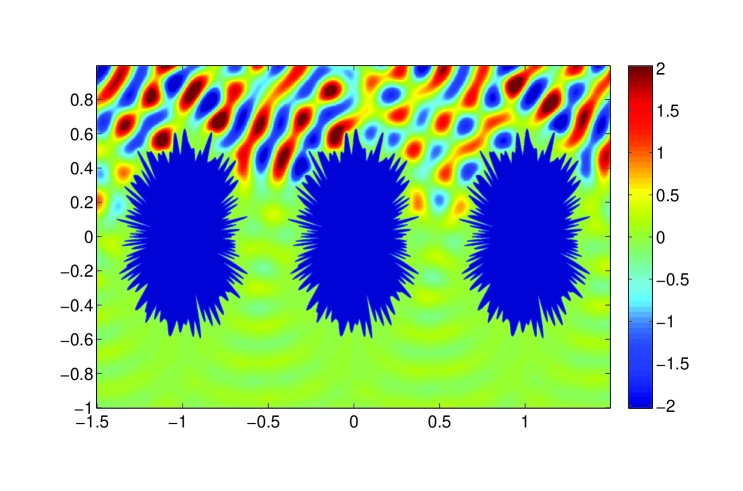
Figure 6.3. Illustration of the total field at a Wood’s anomaly off a collection of complicated obstacles.

Figure 6.4. (a) The flux errors and (b) the outgoing flux fractions for all Bragg modes when solving a Dirichlet problem with $200$ incident angles and $\omega=30$. In (b) each flux fraction is shown in a different gray shade, and the solid blue line separates reflected from transmitted intensity.

6.3. A challenging transmission problem

Prior to the development of the fast direct solver, accurately solving a transmission problem on complicated domains required a lot of computing time. We applied the direct solver to a transmission problem on the domain from section 6.2. With $N=10^{4}$ and all other parameters as in the previous example (thus there are 20241 unknowns), the solver achieves a flux error of $10^{-5}$ in $6$ minutes of pre-computation and $14$ seconds for each block solve. Figure 6.5 illustrates the total field for this example.

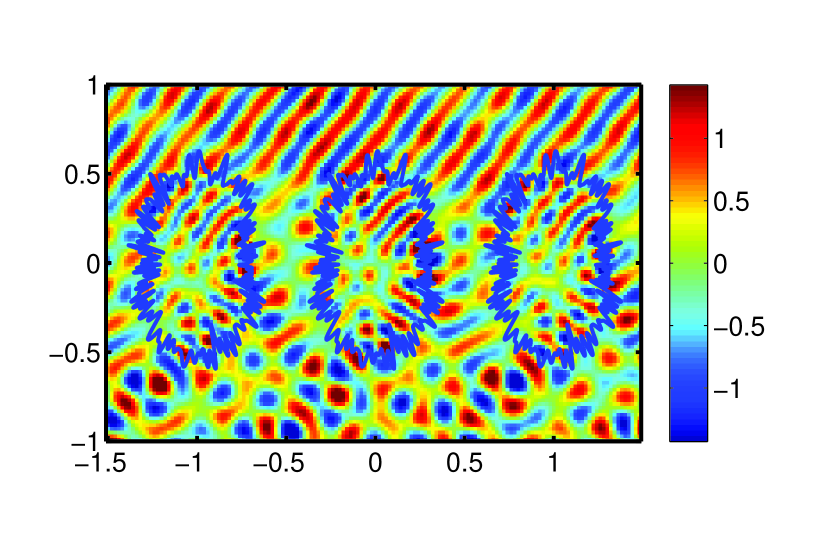
Figure 6.5. Illustration of the total field at a Wood’s anomaly off a collection of complicated obstacles with transmission boundary conditions.

7. Conclusion

This paper presented a fast direct solution technique for grating scattering problems with either Dirichlet or transmission boundary conditions. For low frequency problems on simple domains, the computational cost of the solver scales linearly with the number of discretization points on one obstacle. The example in section 6.2 illustrates that when the obstacle is complicated and the frequency somewhat higher, the direct solver is much faster than an FMM accelerated GMRES, because it handles ill-conditioning. Additionally, the direct solver is very fast for multiple incident angles that occur often in design problems, and this can be further accelerated in the case when many incident angles share a Bloch phase $\alpha$. In one complicated Dirichlet obstacle case which requires $10^{5}$ unknowns to discretize, 200 incident angles are solved in under 6 seconds per incident angle.

Although, for simplicity, we disallowed intersections of ${\partial\Omega}$ with the $L$ and $R$ walls, it would be quite simple to adapt the fast direct solver to the scheme presented in [5, Sec. 6] to handle this case. It would also be relatively easy to generalize the scheme to multi-layer transmission gratings, which are more common in applications. We anticipate creating a fast solver for this case in future work.

References

- [1] B. K. Alpert. Hybrid Gauss-trapezoidal quadrature rules. SIAM J. Sci. Comput., 20:1551–1584, 1999.
- [2] T. Arens. Scattering by biperiodic layered media: The integral equation approach. Habilitation thesis, Karlsruhe, 2010.
- [3] T. Arens, S. N. Chandler-Wilde, and J. A. DeSanto. On integral equation and least squares methods for scattering by diffraction gratings. Commun. Comput. Phys., 1:1010–42, 2006.
- [4] H. A. Atwater and A. Polman. Plasmonics for improved photovoltaic devices. Nature Materials, 9(3):205–213, 2010.
- [5] A. H. Barnett and L. Greengard. A new integral representation for quasi-periodic scattering problems in two dimensions. BIT Numer. Math., 51:67–90, 2011.
- [6] C. P. J. Barty, et al. An overview of LLNL high-energy short-pulse technology for advanced radiography of laser fusion experiments. Nuclear Fusion, 44(12):S266, 2004.
- [7] G. Beylkin, R. Coifman, and V. Rokhlin. Wavelets in numerical analysis. In Wavelets and their applications, pages 181–210. Jones and Bartlett, Boston, MA, 1992.
- [8] Bonnet-BenDhia, A.-S. and F. Starling. Guided waves by electromagnetic gratings and non-uniqueness examples for the diffraction problem. Math. Meth. Appl. Sci., 17:305–338, 1994.
- [9] S. Börm. Efficient Numerical Methods for Non-local Operators: -Matrix Compression, Algorithms and Analysis. European Mathematics Society, 2010.
- [10] O. P. Bruno and M. C. Haslam. Efficient high-order evaluation of scattering by periodic surfaces: deep gratings, high frequencies, and glancing incidences. J. Opt. Soc. Am. A, 26(3):658–668, 2009.
- [11] S. Chandrasekaran and M. Gu. A divide-and-conquer algorithm for the eigendecomposition of symmetric block-diagonal plus semiseparable matrices. Numer. Math., 96(4):723–731, 2004.
- [12] H. Cheng, W. Y. Crutchfield, Z. Gimbutas, G. L., J. Huang, V. Rokhlin, N. Yarvin, and J. Zhao. Remarks on the implementation of the wideband FMM for the Helmholtz equation in two dimensions, volume 408 of Contemp. Math., pages 99–110. Amer. Math. Soc., Providence, RI, 2006.
- [13] H. Cheng, Z. Gimbutas, P. Martinsson, and V. Rokhlin. On the compression of low rank matrices. SIAM Journal of Scientific Computing, 26(4):1389–1404, 2005.
- [14] W. C. Chew. Waves and Fields in Inhomogeneous Media. Wiley-IEEE Press, 1999.
- [15] D. Colton and R. Kress. Integral equation methods in scattering theory. Wiley, 1983.
- [16] D. Colton and R. Kress. Inverse acoustic and electromagnetic scattering theory, volume 93 of Applied Mathematical Sciences. Springer-Verlag, Berlin, second edition, 1998.
- [17] A. Gillman, P. Young, and P. Martinsson. A direct solver with complexity for integral equations on one-dimensional domains. Frontiers of Mathematics in China, 7(2):217–247, 2012.
- [18] A. Gillman, P. Young, and P. G. Martinsson. A direct solver with complexity for integral equations on one-dimensional domains, 2011.
- [19] Z. Gimbutas and L. Greengard. HFMM2D, Fortran code for fast multipole method with Helmholtz kernel in two dimensions (version 20110313), 2011. http://www.cims.nyu.edu/cmcl/fmm2dlib/fmm2dlib.html.
- [20] G. Golub and C. V. Loan. Matrix computations. Johns Hopkins Studies in the Mathematical Sciences. Johns Hopkins University Press, Baltimore, MD, third edition, 1996.
- [21] M. Gu and S. C. Eisenstat. Efficient algorithms for computing a strong rank-revealing QR factorization. SIAM J. Sci. Comput., 17(4):848–869, 1996.
- [22] W. Hackbusch. A sparse matrix arithmetic based on H-matrices; Part I: Introduction to H-matrices. Computing, 62:89–108, 1999.
- [23] S. Hao, P. Martinsson, and P. Young. High-order accurate Nyström discretization of integral equations with weakly singular kernels on smooth curves in the plane, 2011. arXiv.org report #1112.6262.
- [24] J. Helsing. Integral equation methods for elliptic problems with boundary conditions of mixed type. J. Comput. Phys., 228:8892–8907, 2009.
- [25] K. Ho and L. Greengard. A fast direct solver for structured linear systems by recursive skeletonization, 2012. To appear in SIAM J. on Scientific Computing.
- [26] K. V. Horoshenkov and S. N. Chandler-Wilde. Efficient calculation of two-dimensional periodic and waveguide acoustic Green’s functions. J. Acoust. Soc. Amer., 111:1610–1622, 2002.
- [27] S. Kapur and V. Rokhlin. High-order corrected trapezoidal quadrature rules for singular functions. SIAM J. Numer. Anal., 34:1331–1356, 1997.
- [28] A. Klöckner, A. H. Barnett, L. Greengard, and M. O’Neil. Quadrature by expansion: a new method for the evaluation of layer potentials, 2012. submitted.
- [29] R. Kress. Numerical Analysis. Graduate Texts in Mathematics #181. Springer-Verlag, 1998.
- [30] C. M. Linton. Lattice sums for the Helmholtz equation. SIAM Review, 52(4):603–674, 2010.
- [31] P. Martinsson and V. Rokhlin. A fast direct solver for boundary integral equations in two dimensions. J. Comp. Phys., 205(1):1–23, 2005.
- [32] A. Meier, T. Arens, S. N. Chandler-Wilde, and A. Kirsch. A Nyström method for a class of integral equations on the real line with applications to scattering by diffraction gratings and rough surfaces. J. Integral Equations Appl., 12:281–321, 2000.
- [33] E. Michielssen, A. Boag, and W. C. Chew. Scattering from elongated objects: direct solution in operations. IEE Proc. Microw. Antennas Propag., 143(4):277 – 283, 1996.
- [34] R. Model, A. Rathsfeld, H. Gross, M. Wurm, and B. Bodermann. A scatterometry inverse problem in optical mask metrology. J. Phys.: Conf. Ser., 135:012071, 2008.
- [35] P. Morse and H. Feshbach. Methods of theoretical physics, volume 1. McGraw-Hill, 1953.
- [36] M. J. Nicholas. A higher order numerical method for 3-D doubly periodic electromagnetic scattering problems. Commun. Math. Sci., 6(3):669–694, 2008.
- [37] M. A. Peter, M. H. Meylan, and C. M. Linton. Water-wave scattering by a periodic arrya of arbitrary bodies. J. Fluid Mech., 548:237–256, 2006.
- [38] V. Rokhlin. Solution of acoustic scattering problems by means of second kind integral equations. Wave Motion, 5:257–272, 1983.
- [39] N. P. Sergeant, M. Agrawal, and P. Peumans. High performance solar-selective absorbers using coated sub-wavelength gratings. Opt. Express, 18(6):5525–5540, 2010.
- [40] Z. Sheng, P. Dewilde, and S. Chandrasekaran. Algorithms to solve hierarchically semi-separable systems. In System theory, the Schur algorithm and multidimensional analysis, volume 176 of Oper. Theory Adv. Appl., pages 255–294. Birkhäuser, Basel, 2007.
- [41] S. Shipman. Resonant scattering by open periodic waveguides, volume 1 of Progress in Computational Physics (PiCP), pages 7–50. Bentham Science Publishers, 2010.
- [42] P. Starr and V. Rokhlin. On the numerical solution of two-point boundary value problems. II. Comm. Pure Appl. Math., 47(8):1117–1159, 1994.
- [43] Y. Wu and Y. Y. Lu. Analyzing diffraction gratings by a boundary integral equation Neumann-to-Dirichlet map method. J. Opt. Soc. Am. A, 26(11):2444–2451, 2009.