Chiral fluid dynamics with explicit propagation of the Polyakov loop

Abstract

We present a fully dynamical model to study nonequilibrium effects in both the chiral and the deconfinement phase transition. The sigma field and the Polyakov loop as the corresponding order parameters are propagated by Langevin equations of motion. The locally thermalized background is provided by a fluid of quarks and antiquarks. Allowing for an exchange of energy and momentum through dissipative and stochastic processes we ensure that the total energy of the coupled system remains conserved. We study its relaxational dynamics in different quench scenarios and are able to observe critical slowing down as well as the enhancement of long wavelength modes at the critical point. During the fluid dynamical expansion of a hot plasma fireball typical nonequilibrium effects like supercooling and domain formation occur when the system evolves through the first order phase transition.

I Introduction

One of the major goals of heavy-ion physics is to gain firm knowledge about the different phases of strongly interacting matter and the transitions between them. At high temperatures, the chiral symmetry that is broken in the QCD vacuum, is expected to be restored. Furthermore, quarks and gluons might become the relevant degrees of freedom after the transition from hadrons to a deconfined state of matter. From lattice QCD calculations we know that at vanishing baryochemical potential the chiral transition is an analytic crossover Aoki:2006we ; Cheng:2006qk . As recent studies show, there seems to be no direct relation between the chiral restoration and the onset of deconfinement Aoki:2006br ; Aoki:2009sc ; Borsanyi:2010bp . A multitude of effective models have been used to investigate the QCD phase diagram Scavenius:2000qd ; Schaefer:2004en ; Ratti:2005jh ; Schaefer:2007pw ; Sasaki:2007qh ; Skokov:2010uh ; Skokov:2010sf ; Schaefer:2009ui ; Sasaki:2011sd indicating a first order phase transition at large $\mu_{B}$ ending at a critical point (CP). In equilibrium this CP exhibits a divergence in the correlation length of the order parameter. The problem how to locate the CP in the $T$-$\mu_{B}$-plane in heavy-ion collisions was addressed by Stephanov, Rajagopal and Shuryak Stephanov:1998dy ; Stephanov:1999zu for equilibrated systems. They proposed to search for divergences in event-by-event fluctuations of quantities like transverse momentum or particle multiplicity, since the strength of these fluctuations is directly related to the correlation length of the sigma field, the order parameter for the chiral phase transition. However, a priori one cannot expect to reach thermodynamic equilibrium during such a heavy-ion collision, especially near the phase transition where relaxation times become large in comparison to the rapid dynamics of the expanding fireball. Therefore, several additional effects have to be taken into account. Not only is the growth of the correlation length naturally limited by the finite size of the system, but also critical slowing down of the dynamics in the vicinity of the critical point will weaken the expected signals Berdnikov:1999ph . One may try to overcome this difficulty by looking for quantities that are accessible in experiment and more sensitive to the correlation length. Higher cumulants and combinations of them like the kurtosis of conserved quantities such as net baryon number or net charge fulfill this requirement Stephanov:2008qz ; Karsch:2010ck . The fast dynamical evolution of matter through a first order phase transition may exhibit interesting phenomena like supercooling followed by a decay through spinodal decomposition Csernai:1992tj ; Csernai:1995zn ; Scavenius:2000bb ; Randrup:2010ax ; Steinheimer:2012gc ; Chomaz:2003dz or nucleation Mishustin:1998eq . Also an enhancement of soft pions from the decay of a disoriented chiral condensate (DCC) was proposed as a signal for a nonequilibrium chiral phase transition Rajagopal:1993ah ; Biro:1997va ; Xu:1999aq .

Only via thorough theoretical understanding of the processes and effects in dynamical systems undergoing phase transitions one may provide realistic predictions for upcoming experiments with relativistic heavy-ion beams at RHIC Caines:2009yu , CERN SPS Aduszkiewicz:2012fr , FAIR Friman:2011zz and NICA nica:whitepaper .

In Ratti:2005jh , the thermodynamic properties of a Polyakov loop extended Nambu-Jona-Lasinio (PNJL) model were studied and compared with lattice QCD results. The addition of the Polyakov loop to these models improved the behavior of thermodynamic bulk quantities in comparison to the lattice QCD data. A similar extension to the sigma model with constituent quarks was presented in Schaefer:2007pw where a coincidence of the deconfinement and chiral symmetry transition even at finite $\mu_{B}$ was found. An investigation of the phase structure of that model beyond mean-field has been performed in Skokov:2010uh including quantum fluctuations within the functional renormalization group method. This improvement has lead to a quantitative shift in the position of the CP. Furthermore, the authors calculated net-quark number density fluctuations as well as ratios of cumulants as an important means to identify the location of the deconfinement and chiral phase transitions. The relevance of the fermion vacuum loop for such models has been investigated in Skokov:2010sf where it was shown that this term has crucial influence on the phase structure and on physical observables such as net quark number fluctuations. In Schaefer:2009ui an extension of this model to (2+1) flavors together with a comparison with lattice QCD data have been presented. An alternative model using a dilaton field representing a scalar glueball condensate was subject to studies in Sasaki:2011sd . An important step towards the understanding of nonequilibrium effects at the chiral phase transition was done in Sasaki:2007qh , where it was shown that the inclusion of spinodal instabilities yields an enhancement of density fluctuations along the first order transition line. This is in contrast to the usual understanding of thermalized systems where such fluctuations are expected to diverge or grow large only at the CP.

For a better understanding of the processes during a heavy-ion collision nonequilibrium effects have to be taken into account in the framework of a fully dynamical model. A promising ansatz to study the QCD phase transition in such a way is given by a chiral fluid dynamics model that has been developed and extended over more than ten years now Mishustin:1998yc ; Paech:2003fe ; Nahrgang:2011mg ; Nahrgang:2011ll ; arXiv:1105.1962 . In Mishustin:1998yc , the authors introduced a model coupling a relativistic ideal fluid of quarks to the linear sigma model and a scalar glueball condensate. Later in Paech:2003fe this model was used to study the $3+1$ dimensional fluid dynamic expansion of a plasma droplet coupled to the out-of-equilibrium evolution of the long-wavelength modes of the chiral condensate. There the initial fluctuations of the sigma field were propagated deterministically. A self-consistent derivation of the coupled dynamics of fields and fluid together with the local thermodynamic properties of the heat bath was then presented in Nahrgang:2011mg . This step is a crucial improvement as the previous models which propagated the chiral fields using a classical equation of motion neglected relaxational and stochastic processes. As as result, the fields would never relax to their equilibrium state for a given temperature but continue oscillating. In Nahrgang:2011mg , the order parameter of chiral symmetry is propagated by a Langevin equation to include damping and noise in the heat bath of quarks. The quark fluid is propagated according to the equations of ideal hydrodynamics. The relaxational dynamics of the field and the treatment of the finite size of the heat bath were investigated in Nahrgang:2011ll and the first numerical studies of the full expanding system were then presented in arXiv:1105.1962 . A coupling of the linear sigma model to viscous hydrodynamics has been studied in PeraltaRamos:2011wp .

Dynamical models for the Polyakov loop have been proposed in Dumitru:2001 ; Dumitru:2002 ; Fraga:2007gg . In Dumitru:2001 , the authors developed a model for particle production near the deconfinement phase transition due to oscillations in a Polyakov loop condensate. These oscillations were included on the basis of a kinetic term in an effective field theory for a Polyakov loop that is biquadratically coupled to a mesonic field. This idea was further used in Dumitru:2002 , where the authors showed how explosive behavior at the QCD phase transition might be produced by the decay of such a condensate of Polyakov loops. Based on work in Miller:2000pd ; Meisinger:2001cq , a Langevin equation for the deconfinement order parameter for pure SU(2) gauge theory was developed in Fraga:2007gg . It was shown that the dissipative interaction with the medium plays a significant role in the determination of physical time scales.

In the present work, we connect these ideas of a dynamical Polyakov loop with the model of chiral fluid dynamics to take into account effects of the deconfinement phase transition. The newly included deconfinement order parameter is treated as an effective field and propagated by a phenomenological Langevin equation. The suggested model is able to provide a dynamic description of two phase transitions in the background of a fluid dynamically expanding heat bath of quarks. This setup resembles the situation after the collision of two heavy nuclei. In Nahrgang:2011mg the proper nonequilibrium dynamics for the sigma field and the quark fluid have been derived self-consistently for a model without Polyakov loop. The resulting Langevin equation for the sigma field includes two important effects: the damping of the chiral field due to the interaction with the heat bath and the back reaction of the heat bath on the sigma field by stochastic noise. For the dynamics of the Polyakov loop we follow the same idea but on a phenomenological basis as it is currently not possible to derive the dynamics of the Polyakov loop from a consistent field theoretical approach like it has been achieved for the sigma field. With the considered Polyakov loop extended linear sigma model we are able to describe characteristic phenomena at the phase boundary within a dynamical setup.

This article is structured as follows. In section II we present the model of Polyakov loop extended chiral fluid dynamics, where the sigma field and Polyakov loop are coupled to a fluid dynamically propagated heat bath of quarks. After that we consider two different numerical implementations. Section III presents results of relaxational dynamics in a box for several quench scenarios. In section IV we study the evolution of a freely expanding hot plasma undergoing a phase transition. Finally, we present a short summary and outlook in section V.

II Chiral fluid dynamics with a Polyakov loop

II.1 General remarks

Our model extends existing studies of chiral fluid dynamics Mishustin:1998yc ; Paech:2003fe ; Nahrgang:2011mg ; Nahrgang:2011ll ; arXiv:1105.1962 with the Polyakov loop to take into account effects of both the chiral and the deconfinement phase transition. The restoration of ${\rm SU}(N_{f})_{\rm L}\times{\rm SU}(N_{f})_{\rm R}$ chiral symmetry in the high temperature phase can be characterized by the melting of the $\langle\bar{q}q\rangle$ condensate or the sigma field, respectively. For the transition to deconfinement, the Polyakov loop $\ell$ is the quantity of interest. It is defined as the expectation value of the color trace of a thermal Wilson loop:

$$\ell=\frac{1}{N_{c}}\langle tr_{c}{\cal P}\rangle_{\beta}~{},\quad\bar{\ell}=\frac{1}{N_{c}}\langle tr_{c}{\cal P^{\dagger}}\rangle_{\beta}~{},$$ (1)

where the operator ${\cal P}$ is defined as

$${\cal P}=P\exp\left(ig_{\rm s}\int_{0}^{\beta}\mathrm{d}\tau A_{0}\right)~{}.$$ (2)

Here, $P$ stands for path ordering, $A_{0}$ denotes the temporal component of the Euclidean color gauge field, $g_{\rm s}$ the strong coupling constant and $\beta=1/T$ is the inverse temperature. The expectation value of $\ell$ is related to the free energy $F_{q}(\vec{x})$ of an infinitely heavy test quark at spatial position $\vec{x}$ via

$$\langle\ell(\vec{x})\rangle=\mathrm{e}^{-\beta F_{q}(\vec{x})}~{}.$$ (3)

In the confined phase, this free energy diverges and therefore $\langle\ell\rangle$ vanishes whereas it takes some finite value in the deconfined phase. In the limit of infinitely heavy quarks, QCD is invariant under $Z(N_{c})$ center symmetry transformations of the $SU(N_{c})$ color gauge group. The Polyakov loop transforms as

$$\ell\rightarrow z\ell~{},\quad z\in Z(N_{c})~{},$$ (4)

with the consequence that the confined phase is center symmetric while this symmetry is spontaneously broken in the deconfined phase. In the presence of dynamical quarks, the Polyakov loop is always non-zero as the free energy of a test quark does not diverge anymore. Nevertheless, $\langle\ell\rangle$ may still serve to characterize the transition between the two phases.

II.2 The model

For our studies we use the Polyakov loop extended quark meson model Schaefer:2007pw . The Lagrangian reads

$${\cal L}=\overline{q}\left[i\left(\gamma^{\mu}\partial_{\mu}-ig_{\rm s}\gamma^{0}A_{0}\right)-g\left(\sigma+i\gamma_{5}\vec{\tau}\cdot\vec{\pi}\right)\right]q+\frac{1}{2}\left(\partial_{\mu}\sigma\right)^{2}+\frac{1}{2}\left(\partial_{\mu}\vec{\pi}\right)^{2}-U\left(\sigma,\vec{\pi}\right)-{\cal U}(\ell,\bar{\ell})~{},$$ (5)

where $q=(u,d)$ is the constituent quark field, so $N_{f}=2$, and $\sigma$ the mesonic sigma field. For our simulations around the phase transition we utilize a fixed strong coupling constant of $\alpha_{\rm s}=g_{\rm s}^{2}/(4\pi)=0.3$. As we are only interested in the behavior of the order parameters, we neglect fluctuations of the pionic degrees of freedom and keep their values fixed at the vanishing expectation value $\vec{\pi}=\langle\vec{\pi}\rangle=0$ for all times. The potential for the sigma field reads

$$U\left(\sigma\right)=\frac{\lambda^{2}}{4}\left(\sigma^{2}-\nu^{2}\right)^{2}-h_{q}\sigma-U_{0}~{}.$$ (6)

The chiral symmetry of the Lagrangian (5) is explicitly broken by the term $h_{q}$ in the potential (6) taking into account the finite quark masses. The parameters in (6) are chosen such that chiral symmetry is spontaneously broken in the vacuum, where $\langle\sigma\rangle=f_{\pi}=93$ MeV, the pion decay constant. The explicit symmetry breaking term is $h_{q}=f_{\pi}m_{\pi}^{2}$ with the pion mass $m_{\pi}=138$ MeV. These requirements lead to $\nu^{2}=f_{\pi}^{2}-m_{\pi}^{2}/\lambda^{2}$. Choosing $\lambda^{2}=19.7$ yields a realistic vacuum sigma mass $m_{\sigma}^{2}=2\lambda^{2}f_{\pi}^{2}+m_{\pi}^{2}\approx 600$ MeV. The constant term $U_{0}=m_{\pi}^{4}/(4\lambda^{2})-f_{\pi}^{2}m_{\pi}^{2}$ is chosen such that the potential energy vanishes in the ground state. The quark-meson coupling constant is fixed by the requirement to reproduce the constituent quark mass in vacuum, $g=m_{q}/f_{\pi}=3.3$.

The temperature dependent Polyakov loop potential is chosen in a polynomial form Schaefer:2007pw ; Ratti:2005jh ; Pisarski:2000eq .

$$\frac{{\cal U}}{T^{4}}\left(\ell,\bar{\ell}\right)=-\frac{b_{2}(T)}{4}\left(\left|\ell\right|^{2}+\left|\bar{\ell}\right|^{2}\right)-\frac{b_{3}}{6}\left(\ell^{3}+\bar{\ell}^{3}\right)+\frac{b_{4}}{16}\left(\left|\ell\right|^{2}+\left|\bar{\ell}\right|^{2}\right)^{2}~{}.$$ (7)

At non-vanishing $\mu_{B}$, this parametrization yields an unphysical behavior in the Polyakov loop susceptibilities which become negative in a broad temperature range Sasaki:2006ww . One can cure this problem by augmenting this effective potential with a logarithmic term to account for the Haar measure in the group integral Sasaki:2006ww ; Ratti:2007jf ; Roessner:2006xn . As we will restrict our numerical studies to the case of zero baryochemical potential, we can ignore this issue for the present investigation.

The coefficients in (7) are fixed to reproduce thermodynamic results from lattice QCD simulations in the pure gauge sector. We use parametrizations proposed in Ratti:2005jh ; Ratti:2004ra ; Heinzl:2005xv ; deForcrand:2001nd ; Wozar:2006fi

$$b_{2}(T)=a_{0}+a_{1}\left(\frac{T_{0}}{T}\right)+a_{2}\left(\frac{T_{0}}{T}\right)^{2}+a_{3}\left(\frac{T_{0}}{T}\right)^{3}$$ (8)

with $a_{0}=6.75$, $a_{1}=-1.95$, $a_{2}=2.625$, $a_{3}=-7.44$ and two temperature independent coefficients $b_{3}=0.75$ and $b_{4}=7.5$. The potential (7) has a first-order phase transition at a critical temperature of $T_{0}=270$ MeV. However, in the presence of dynamical quarks this transition temperature gets lower due to the increased number of degrees of freedom and reduced dynamical scale. The proper $N_{f}$- and $\mu_{B}$-dependence of $T_{0}$ has been investigated in Herbst:2010rf . For two flavors and vanishing baryochemical potential, $T_{0}$ reduces to a value of $208$ MeV.

The effective thermodynamic potential that we need for describing the dynamics of $\sigma$ and $\ell$ and for the local equilibrium properties of the quarks is given by

$$V_{\rm eff}=-\frac{T}{V}\ln{\cal Z}=U+{\cal U}+\Omega_{q\bar{q}}~{}.$$ (9)

The partition function ${\cal Z}$ of our system can be written as a path integral over the quarks, antiquarks, mesons and the temporal component of the color gauge field. Integrating out the quark degrees of freedom, which will constitute the heat bath, we obtain the grand canonical potential $\Omega_{q\bar{q}}$. At $\mu_{B}=0$, $\ell=\bar{\ell}$ and in the mean-field approximation it is Schaefer:2007pw

$$\Omega_{q\bar{q}}=-4N_{f}T\int\frac{\mathrm{d}^{3}p}{(2\pi)^{3}}\ln\left[1+3\ell\mathrm{e}^{-\beta E}+3\ell\mathrm{e}^{-2\beta E}+\mathrm{e}^{-3\beta E}\right]~{}.$$ (10)

Here $E=\sqrt{p^{2}+g^{2}\sigma^{2}}$, the energy of the quarks, their mass being generated dynamically by the sigma field. The integrand contains contributions from one-, two- and three-quark states, the first two being proportional to $\ell$. This means that for vanishing value of the Polyakov loop only three-quark states contribute, while the amount of one- and two-quarks gets larger with growing $\ell$. This is called “statistical confinement” Morita:2011jv . In (10), we omit the zero-temperature contribution to $\Omega_{q\bar{q}}$ which can partly be renormalized into the parameters $\lambda^{2}$ and $\nu^{2}$, leaving a logarithmic term depending on the renormalization scale and the effective quark mass. This term may have crucial influence on the phase structure of the model Skokov:2010sf ; Mocsy:2004ab . However, as the mean-field approximation provides us with the desired phase transition already Scavenius:2000qd , we neglect this term and its effects in the following. In order to simplify the calculations and for a first qualitative study we follow the same strategy as in Paech:2003fe ; Nahrgang:2011mg ; Nahrgang:2011ll . Varying the coupling strength $g$ one can tune the characteristic shape of the effective potential $V_{\rm eff}$ at $\mu_{B}=0$ and by that the type of transition: For $g=4.7$ we see two degenerate minima $(\sigma=9~{}\rm{MeV},\ell=0.40)$ and $(\sigma=81~{}\rm{MeV},\ell=0.22)$ at the transition temperature of $T_{c}=172.9$ MeV, see fig. 1a. While for $g=3.52$ we have only one single minimum $(\sigma=49~{}\rm{MeV},\ell=0.43)$ at $T_{c}=180.5$ MeV, where the potential is very broad and flat as shown in fig. 1b. This resembles a CP. Note that in principle one has to choose $g$ such that the product $g\sigma$ in vacuum reproduces the constituent quark mass, which leads to a value of $g=3.3$.

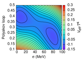
(a)

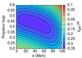
(b)

Figure 1: 1a Effective potential for $g=4.7$, corresponding to a first order phase transition at $T_{c}=172.9$ MeV. 1b Effective potential for $g=3.52$, corresponding to a CP scenario at $T_{c}=180.5$ MeV.

II.3 The equations of motion

In Nahrgang:2011mg we have derived the coupled dynamics of the sigma field and the quark fluid self-consistently with the two particle irreducible (2PI) effective action for an analogous model without Polyakov loop. The description of nonequilibrium processes can be achieved via Langevin equations. This has been extensively done in a quantum field theoretical framework for $\phi^{4}$ theory Morikawa:1986rp ; Gleiser:1993ea ; Boyanovsky:1996xx ; Greiner:1996dx , gauge theories Bodeker:1995pp ; Son:1997qj and $\mathcal{O}(N)$ chiral models Rischke:1998qy . Here, a splitting between the long- and short-wavelength modes of the sigma field was assumed and the relaxational dynamics of the soft modes in the heat bath of hard modes was derived within the influence functional formalism. Utilizing a chiral model with constituent quarks, we assumed a different splitting. Taking the quarks as the environmental degrees of freedom and the sigma as the relevant degrees one can calculate the 2PI effective action by integrating over the Keldysh contour. Out of that we were able to derive a Langevin equation of motion containing friction and noise

$$\partial_{\mu}\partial^{\mu}\sigma+\eta_{\sigma}(T)\partial_{t}\sigma+\frac{\partial V_{\rm eff}}{\partial\sigma}=\xi_{\sigma}~{}.$$ (11)

The damping coefficient $\eta_{\sigma}$ is temperature dependent and responsible for the transfer of energy-momentum to the heat bath. It arises from the $\sigma\leftrightarrow q\bar{q}$ process and is non-vanishing wherever this decay is kinematically possible. In Nahrgang:2011mg we derived its explicit form in the $\left|\vec{k}\right|=0$ limit which is sufficient as we are interested mainly in the fluctuations of the soft modes. For $m_{\sigma}>2m_{q}$ it is given by

$$\eta_{\sigma}=\frac{12g^{2}}{\pi}\left[1-2n_{\rm F}\left(\frac{m_{\sigma}}{2}\right)\right]\frac{\left(\frac{m_{\sigma}^{2}}{4}-m_{q}^{2}\right)^{\frac{3}{2}}}{m_{\sigma}^{2}}~{},$$ (12)

with $m_{\sigma}$ being the pole mass of the sigma field. While the screening mass, defined as the curvature of the effective potential at the equilibrium value, vanishes at the CP, this is not in general true for the pole mass. However, we use

$$m_{\sigma}^{2}=\left.\frac{\partial^{2}V_{\rm eff}}{\partial\sigma^{2}}\right|_{\sigma=\sigma_{eq},\,\ell=\ell_{eq}}$$ (13)

as an approximation to the proper pole mass for equation (12). This ansatz is justified as the pole mass has a minimum at the transition temperature for a crossover scenario just like the screening mass. A consistent calculation is possible by considering the dispersion relations for different types of excitations.

For the damping below the phase transition we choose $\eta_{\sigma}=2.2/{\mathrm{f}m}$ Biro:1997va to account for the $\sigma\leftrightarrow\pi\pi$ reaction whenever it is kinematically allowed. Fig. 2 shows $\eta_{\sigma}$ as a function of temperature for both transition scenarios. Due to its perturbative derivation, the damping coefficient is rather high, especially for the first order transition. The only region where it vanishes is around $T_{c}$ for the CP, where the sigma becomes light enough so that $m_{\sigma}<2m_{q},\ 2m_{\pi}$. The stochastic noise field in the equation of motion (11) has a vanishing expectation value $\langle\xi_{\sigma}\rangle=0$. To complete this part we derive a dissipation-fluctuation-relation that connects the damping coefficient to the correlator of the stochastic noise field and ensures the relaxation to the proper equilibrium state.

$$\langle\xi_{\sigma}(t,\vec{x})\xi_{\sigma}(t^{\prime},\vec{x}^{\prime})\rangle=\frac{1}{V}\delta(t-t^{\prime})\delta(\vec{x}-\vec{x}^{\prime})m_{\sigma}\eta_{\sigma}\coth\left(\frac{m_{\sigma}}{2T}\right)~{}.$$ (14)

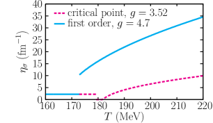
Figure 2: Damping coefficient for the sigma field as a function of temperature, for a CP and a first order transition scenario.

The temperature, the mass of the sigma field, the damping and the noise field in (14) are local quantities which may vary between different positions on the spatial grid.

The derivation of the equation of motion for the Polyakov loop $\ell$ is more problematic because $\ell$ is defined in the Euclidean space and it is not completely clear how to propagate it in real time. In Dumitru:2001 a kinetic term for the Polyakov loop has been included in the Lagrangian:

$$\mathcal{L}\rightarrow\mathcal{L}+\frac{N_{c}}{g_{\rm s}^{2}}\left|\partial_{\mu}\ell\right|^{2}T^{2}~{}.$$ (15)

It was proposed that production of pions near the phase transition is driven by oscillations of the Polyakov loop. Only in the region around $T_{c}$ the Polyakov loop is light, allowing large fluctuations and thus particle production. As the Polyakov loop operator is a phase in color space and therefore $\ell$ a pure number, dimensions in an effective Lagrangian can only be made up by powers of the temperature $T$. However, the temperature in our model is space and time dependent, so the Euler-Lagrange equation for $\ell$ would contain derivative terms of $T$ that might lead to unphysical behavior.

For our present model we follow a different strategy formulated in Landau:1983 . If the order parameter is out of equilibrium, then relaxational processes towards its thermodynamic equilibrium value will occur. The velocity of relaxation is then proportional to the derivative of the effective potential with respect to the order parameter. Analogous to the sigma field we include fluctuations of the Polyakov loop with a stochastic noise term for which $\langle\xi_{\ell}\rangle=0$:

$$\eta_{\ell}\partial_{t}\ell T^{2}+\frac{\partial V_{\rm eff}}{\partial\ell}=\xi_{\ell}~{},$$ (16)

$$\langle\xi_{\ell}(t,\vec{x})\xi_{\ell}(t^{\prime},\vec{x}^{\prime})\rangle T^{2}=\frac{1}{V}\delta(t-t^{\prime})\delta(\vec{x}-\vec{x}^{\prime})2\eta_{\ell}T~{}.$$ (17)

Equation (17) assumes Gaussian and Markovian noise as it was used in Fraga:2007gg . In contrast to the sigma field it is not clear how to derive a damping for the Polyakov loop in a field theoretical manner as the fermionic part of the Lagrangian contains interaction with the $A_{0}$ color gauge field but not directly with $\ell$. Therefore we chose a ‘reasonable’ value of $\eta_{\ell}=5/fm$, although the results are not sensitive to it. We will further comment on this later.

II.4 Propagation of the quark fluid

The propagation of the quark fluid is governed by the equations of ideal relativistic fluid dynamics

$$\partial_{\mu}\left(T^{\mu\nu}_{q}+T^{\mu\nu}_{\sigma}+T^{\mu\nu}_{\ell}\right)=0~{}.$$ (18)

We require energy-momentum conservation for the system as a whole, its energy-momentum tensor being split into quark, sigma and Polyakov loop parts. In Nahrgang:2011mg we were able to derive self-consistently an approximate expression for the quark and sigma contribution. For the quarks we obtained the energy-momentum tensor of an ideal fluid, the contribution of the sigma field can be expressed as

$$\partial_{\mu}T^{\mu\nu}_{\sigma}=\left(-\frac{\partial\Omega_{q\bar{q}}}{\partial\sigma}-\eta_{\sigma}\partial_{t}\sigma\right)\partial^{\nu}\sigma~{}.$$ (19)

Assuming the same structure and effects for the Polyakov loop contribution, we end up with

$$\partial_{\mu}T^{\mu\nu}_{\ell}=\left(-\frac{\partial\Omega_{q\bar{q}}}{\partial\ell}-\eta_{\ell}\partial_{t}\ell T^{2}\right)\partial^{\nu}\ell~{}.$$ (20)

As explained in Nahrgang:2011mg , these terms cannot account for the average energy transfer from the heat bath to the fields caused by the stochastic noise fields $\xi_{\sigma}$ and $\xi_{\ell}$. The equation of state $p=p(e)$ is obtained and tabulated from the thermodynamic relations

$$p(\sigma,\ell,T) = -\Omega_{q\bar{q}}(\sigma,\ell,T)~{},$$ (21)

$$e(\sigma,\ell,T) = T\frac{\partial p(\sigma,\ell,T)}{\partial T}-p(\sigma,\ell,T)~{}.$$ (22)

A simple relation for $p(e)$ cannot be obtained as $\sigma$ and $\ell$ are propagated explicitly and can be out of equilibrium and the pressure as well as the energy density of the quarks depend explicitly on the local values of these fields.

III Equilibration in a box

In this section we study the relaxational behavior of the order parameters in a box of finite size after several temperature quenches. The aim is to give estimates and compare relaxation times near and far away from the transition point for a first order and a CP scenario. Furthermore we investigate fluctuations during and after the equilibration process.

III.1 Numerical implementation

We solve the equations of motion for the fields and the quark fluid on a fixed spatial cube of size $L^{3}$ where $L=N\Delta x$ with $N$ equal to the number of cells in each direction and the grid spacing $\Delta x=0.2$ fm. The fluid dynamic equations (18) are solved using the full (3+1)d SHarp And Smooth Transport Algorithm (SHASTA) ideal fluid dynamic code Rischke:1995ir ; Rischke:1995mt . To ensure numerical stability we use a time step of $\Delta t=0.4\cdot\Delta x=0.08$ fm.

Rewriting the equation of energy and momentum conservation for the coupled system with a source term $S^{\nu}$ for the fluid we obtain

$$\partial_{\mu}T^{\mu\nu}_{q}=-\partial_{\mu}\left(T^{\mu\nu}_{\sigma}+T^{\mu\nu}_{\ell}\right)=S^{\nu}~{}.$$ (23)

After performing the fluid dynamical step for vanishing $S^{\nu}$ in the standard fashion, we subtract the sources from the energy and momentum density in the global rest frame of the fluid. This is especially interesting for an expanding medium and has been successfully implemented in previous studies of chiral fluid dynamics simulations without a Polyakov loop Nahrgang:2011ll ; arXiv:1105.1962 . As will be shown later, this enables us to conserve the total energy for our Polyakov loop extended model, see section IV.2.

To implement the source term in the numerical simulation we apply the same strategy as in arXiv:1105.1962 . Equations (19) and (20) provide us with the energy density dissipated into the heat bath.

$$\Delta e_{\rm{diss}}=\left[\left(\frac{\partial\Omega_{q\bar{q}}}{\partial\sigma}+\eta_{\sigma}\partial_{t}\sigma\right)\partial_{t}\sigma+\left(\frac{\partial\Omega_{q\bar{q}}}{\partial\ell}+\eta_{\ell}\partial_{t}\ell T^{2}\right)\partial_{t}\ell\right]\Delta t~{}.$$ (24)

The energy transfer due to stochastic fluctuations $\Delta e_{\rm fluc}$ can be calculated by comparing this term to the numerically obtained energy difference in the sigma and Polyakov loop fields before and after each time step. The energy density of the sigma field is given by the sum of a potential, kinetic and fluctuation term while for the Polyakov loop it is associated only with the potential energy due to the lack of a kinetic term in the Lagrangian.

$$e_{\sigma} = U(\sigma)+\frac{1}{2}\left(\frac{\partial\sigma}{\partial t}\right)^{2}+\frac{1}{2}\left(\vec{\nabla}\sigma\right)^{2}~{},$$ (25)

$$e_{\ell} = {\cal U}(\ell)~{}.$$ (26)

Altogether this gives us the zero component of the source term

$$S^{0}=\frac{1}{\Delta t}\left(\Delta e_{\rm diss}+\Delta e_{\rm fluc}\right)~{}.$$ (27)

The spatial components accounting for momentum transfer are calculated in an analogous fashion. The momentum transfer due to dissipative processes is given by

$$\Delta\vec{M}_{\rm diss}=\left[\left(\frac{\partial\Omega_{q\bar{q}}}{\partial\sigma}+\eta_{\sigma}\partial_{t}\sigma\right)\vec{\nabla}\sigma+\left(\frac{\partial\Omega_{q\bar{q}}}{\partial\ell}+\eta_{\ell}\partial_{t}\ell T^{2}\right)\vec{\nabla}\ell\right]\Delta t~{},$$ (28)

and $\Delta\vec{M}_{\rm fluc}$ is obtained by comparing this to the change in the momentum density of the fields which is vanishing for the Polyakov loop.

$$\vec{M}_{\sigma} = \partial_{t}\sigma\vec{\nabla}\sigma~{},$$ (29)

$$\vec{M}_{\ell} = 0~{}.$$ (30)

This gives us the spatial part of the source term

$$\vec{S}=\frac{1}{\Delta t}\left(\Delta\vec{M}_{\rm diss}+\Delta\vec{M}_{\rm fluc}\right)~{}.$$ (31)

The Langevin equations of motion for the fields $\sigma$ and $\ell$ are solved using a staggered leap-frog algorithm, cf. CassolSeewald:2007ru . For this algorithm the time step is chosen smaller than for the propagation of the fluid. We use a four times smaller $\Delta t$ of $0.1\cdot\Delta x=0.02$ fm. I. e., four consecutive time steps of calculation for the fields are performed with the same fluid background, followed by one step for the fluid propagation. After that, the local temperatures $T(\vec{x})$ are adjusted in each cell via a root finder of

$$e_{\rm fluid}(\vec{x})-e\{\sigma(\vec{x}),\ell(\vec{x}),T(\vec{x})\}=0~{}.$$ (32)

These local temperatures then enter the local potentials (7), (10) and consequently the equations of motion (11) and (16) which are then used in the next time step for the propagation of the order parameter fields.

III.2 Results

We are interested in the investigation of relaxational processes of the coupled system of fields and fluid after a temperature quench. Using a cubic $64^{3}$ grid with periodic boundary conditions we set the temperature $T_{\rm ini}$ uniformly to a value above $T_{c}$ and then initialize the sigma and Polyakov loop field at their equilibrium values including thermal fluctuations with a variance given by

$$\langle\delta\sigma^{2}\rangle = \frac{T}{V}\frac{1}{m_{\sigma}^{2}}~{},$$ (33)

$$\langle\delta\ell^{2}\rangle = \frac{T}{V}\frac{1}{m_{\ell}^{2}}~{}.$$ (34)

Here we have defined the mass of the Polyakov loop $m_{\ell}$ analogously to the sigma mass as

$$m_{\ell}^{2}=\left.\frac{1}{T^{2}}\frac{\partial^{2}V_{\rm eff}}{\partial\ell^{2}}\right|_{\sigma=\sigma_{eq},\,\ell=\ell_{eq}}~{}.$$ (35)

We then quench the temperature to various values $T<T_{c}$ and initialize the quark heat bath by calculating its energy density and pressure out of the given quantities $T$, $\sigma$, $\ell$ via equations (21) and (22). After that we let the system evolve according to equations (11), (16) and (23). Fields and fluid now influence each other in the following way: The amount of energy that the fields lose through damping gets transferred to the fluid which causes an adjustment of the temperature on account of equation (32). This new temperature then reshapes the thermodynamic potential that influences the dynamics of the fields. In this kind of box calculations pressure gradients in the fluid are small, so we expect the dynamics to be governed by the fields.

We are now interested in the relaxational behavior of the sigma field and the Polyakov loop comparing volume averages over all cells of the box as they evolve in time for different quench temperatures and two transition scenarios. The volume averages in a single event are defined as

$$\langle\sigma\rangle=\frac{1}{N^{3}}\sum_{ijk}\sigma_{ijk}~{},\ \langle\ell\rangle=\frac{1}{N^{3}}\sum_{ijk}\ell_{ijk}~{},$$ (36)

where $\sigma_{ijk}$ ($\ell_{ijk}$) is the instantaneous value of the sigma field (Polyakov loop) in a cell with coordinates i, j, k. These values are furthermore averaged over $N_{e}$ events with different noise configurations

$$\overline{\langle\sigma\rangle}=\frac{1}{N_{e}}\sum_{n=1}^{N_{e}}\langle\sigma\rangle_{n}~{},\ \overline{\langle\ell\rangle}=\frac{1}{N_{e}}\sum_{n=1}^{N_{e}}\langle\ell\rangle_{n}~{}.$$ (37)

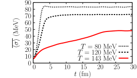
(a)

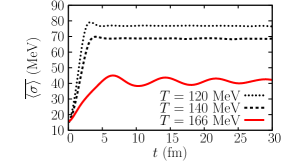
(b)

Figure 3: 3a Equilibration of the sigma field for several quench temperature $T<T_{c}$ through the first order transition. The barrier between the minima in the potential increases the relaxation time when the system relaxes near $T_{c}=172.9$ MeV. We chose $T_{\rm ini}=180$ MeV. 3b Equilibration of the sigma field for several quench temperature $T<T_{c}$ through the CP. Critical slowing down delays the dynamics and causes oscillations around the flat minimum when the system relaxes near $T_{c}=180.5$ MeV. We chose $T_{\rm ini}=186$ MeV.

Results for both transition scenarios are shown in fig. 3. They show the evolution of the noise and volume averaged value of the sigma field in time for different quenching temperatures $T$. The solid curves indicate the case where the system relaxes near the corresponding transition temperature. In both cases the dynamics is slowed down, however for different reasons. At the first order phase transition the barrier that separates minima near $T_{c}$ is responsible for a significant delay in the relaxation dynamics. For the second order transition we observe critical slowing down. This is inherent in the model due to the vanishing of the damping coefficient around the critical temperature that causes the system to oscillate around the equilibrium state and prolong the relaxation time up to infinity.

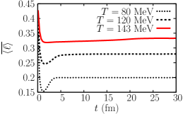
(a)

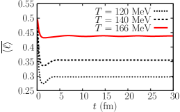
(b)

Figure 4: 4a Equilibration of the Polyakov loop for several temperature quenches $T<T_{c}$ through the first order transition. We chose $T_{\rm ini}=180$ MeV. 4b Equilibration of the Polyakov loop for several temperature quenches $T<T_{c}$ through the CP. We chose $T_{\rm ini}=186$ MeV.

The average values of the Polyakov loop as a function of time are shown in fig. 4. Here we find again a prolongation of the relaxation time near the first order phase transition where the average value is slowly growing until $t=25$ fm while for the other quenching temperatures, the system is equilibrated after $5$ fm. For a CP scenario, we observe the same effect than for the sigma field: critical slowing down near the transition temperature, nevertheless with a small amplitude.

We performed these simulations with various damping coefficients for the Polyakov loop $\eta_{\ell}$ ranging from $1/{\rm fm}$ up to $10/{\rm fm}$. A significant difference in the relaxational behavior could only be observed in the case where the system equilibrated near the first order phase transition where a larger value of $\eta_{\ell}$ caused a larger relaxation time. In all other cases the results are not sensitive to the choice of damping. Therefore we may consider our choice of $\eta_{\ell}=5/{\rm fm}$ as justified, especially for the case of an expanding hot medium, which we finally aim to describe.

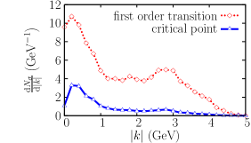
(a)

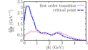
(b)

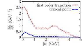
(c)

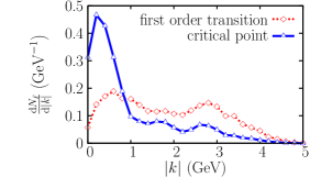
(d)

Figure 5: 5a Intensity of sigma fluctuations during the transition process at $t=12$ fm (first order) and $t=3$ fm (CP). 5b Intensity of sigma fluctuations after equilibration at $t=24$ fm. In the CP scenario we find an enhancement of the soft modes. 5c Intensity of Polyakov loop fluctuations during the transition process at $t=12$ fm (first order) and $t=3$ fm (CP). 5d Intensity of Polyakov loop fluctuations after equilibration at $t=24$ fm. In the CP scenario we find an enhancement of the soft modes.

The fluctuations of the order parameters can be analyzed by calculating their intensity $N_{\sigma}$ and $N_{\ell}$. For the sigma field this quantity is given by Abada:1996bw ; AmelinoCamelia:1997in ; arXiv:1105.1962

$$\frac{\mathrm{d}N_{\sigma}}{\mathrm{d}^{3}k}=\frac{a_{k}^{\dagger}a_{k}}{(2\pi)^{3}2\omega_{k}}=\frac{\omega_{k}^{2}|\delta\sigma_{k}|^{2}+|\partial_{t}\sigma_{k}|^{2}}{(2\pi)^{3}2\omega_{k}}~{},$$ (38)

where $a_{k}^{\dagger}$ and $a_{k}$ are the Fourier coefficients of the expansion of the sigma field around its equilibrium value $\delta\sigma=\sigma-\sigma_{\rm eq}$ and of the conjugate momentum field $\partial_{t}\sigma$. The energy of the $k$-th mode is $\omega_{k}=\sqrt{\vec{k}^{2}+m_{\sigma}^{2}}$. We use an analogous definition for the Polyakov loop

$$\frac{\mathrm{d}N_{\ell}}{\mathrm{d}^{3}k}=T^{2}\frac{\omega_{k}^{2}|\delta\ell_{k}|^{2}+|\partial_{t}\ell_{k}|^{2}}{(2\pi)^{3}2\omega_{k}}$$ (39)

with $\omega_{k}=\sqrt{\vec{k}^{2}+m_{\ell}^{2}}$, although this field formally has no kinetic energy term (see discussion at the end of section II.3). In equilibrium the quantities $N_{\sigma}$, $N_{\ell}$ may be interpreted as particle numbers, but to avoid confusion we call them ‘intensities of fluctuations’. Several histograms of $N_{\sigma}$ and $N_{\ell}$ as a function of the wave number $|k|$ evaluated at different times are shown in figs. 5a, 5b for the sigma field and figs. 5c, 5d for the Polyakov loop. The figures on the left hand side show the intensity at early times during the transition process. We see that here fluctuations at the first order transition are clearly enhanced compared to the CP scenario. On the right hand side the intensities are shown for the time $t=24$ fm after the system has equilibrated. Here we see that the long wavelength modes of both order parameters are enhanced at the CP, a typical and well-known critical phenomenon Stephanov:1999zu .

IV Dynamics in an expanding medium

Here we are interested in the coupled dynamics of a system which is not confined in a box but freely expands into vacuum, similar to what happens after a heavy-ion collision. We study the relaxational behavior of the sigma field and Polyakov loop during the nonequilibrium evolution and investigate the influence of energy-momentum exchange on the temperature evolution in both transition scenarios.

IV.1 Numerical implementation

For this simulation we use a $128^{3}$ grid and initialize in its center a droplet which is ellipsoidal in the x-y-plane and uniform in z-direction. This resembles the almond shape of the overlap region of two colliding nuclei. The droplet has a temperature of $T_{\rm ini}=200$ MeV, well above both transition temperatures and is smoothed by a Woods-Saxon distribution function at its edges:

$$T(\vec{x},t=0)=\frac{T_{\rm ini}}{\big{(}1+\exp[(\tilde{r}-\tilde{R})/\tilde{a}]\big{)}\big{(}1+\exp[(\left|z\right|-l_{z})/\tilde{a}]\big{)}}~{}.$$ (40)

Here, $\tilde{r}=\sqrt{x^{2}+y^{2}}$, $\tilde{a}=0.6$ fm is the thickness of the transition layer to vacuum and

$$\tilde{R}=\begin{cases}\frac{ab\tilde{r}}{\sqrt{b^{2}x^{2}+a^{2}y^{2}}},&\tilde{r}\neq 0\\ a,&\tilde{r}=0\end{cases}~{}.$$ (41)

The ellipsoidal parameters are chosen as $a=r_{A}-\tilde{b}/2$ and $b=\sqrt{r_{A}^{2}-\tilde{b}/4}$, $r_{A}=6.5$ fm denoting the radius of the two nuclei and $\tilde{b}=6$ fm the impact parameter. The extent in z-direction is $2l_{z}=12$ fm. The sigma and Polyakov loop fields are initialized with their respective equilibrium distribution, then the energy density and pressure of the quark fluid are calculated. We choose an initial velocity profile with $v_{z}(\vec{x},t)=|z|/l_{z}\cdot v_{\rm max}$ with $v_{\rm max}=0.2$. The transverse velocities $v_{x}$ and $v_{y}$ are set to zero in the beginning.

IV.2 Energy conservation

We let the system expand by full $3+1$ dimensional fluid dynamics and check the conservation of the total energy throughout the evolution. The energy of the sigma and Polyakov loop field are given by (25) and (26). Fig. 6 shows the total energy and the partial energies of the quark fluid, the sigma field and the Polyakov loop during the fluid dynamical expansion. For both scenarios the total energy is well conserved until the quark fluid reaches the edges of the computational grid after $8$ fm.

(a)

(b)

Figure 6: 6a The total energy as composed of the energy of the sigma field, Polyakov loop and the quark fluid of an expanding system for a first order transition scenario. 6b The total energy as composed of the energy of the sigma field, Polyakov loop and the quark fluid of an expanding system for a scenario with a CP.

IV.3 Supercooling and reheating

During the fluid dynamic expansion we extract the average temperature $\langle T\rangle$, sigma field $\langle\sigma\rangle$ and Polyakov loop $\langle\ell\rangle$ in a central cubic volume of $1\rm{fm}^{3}$ inside the hot matter as a function of time. The results are shown in fig. 7a for the first order transition and in fig. 7b for a scenario with a CP. One can observe significant differences in the evolution of the average temperatures between both scenarios: For the case of the first order transition, fig. 7a, a reheating occurs after $6$ fm as a consequence of the formation of a supercooled phase below the transition temperature. We see that as the average temperature falls below $T_{c}$, the average values of the sigma field and Polyakov loop remain close to their high temperature values around $\sigma/f_{\pi}=0.1$ and $\ell=0.4$. This supercooled state decays after about $2$ fm to the global minimum and transfers its energy into the fluid which consequently causes an increase in the average temperature.

For the CP scenario, fig. 7b, no reheating effect is observed. The temperature decreases monotonically with only a small plateau well below the transition temperature where the dynamics slightly slows down due to the flat shape of the effective potential. The evolution of the averaged fields, especially for $\langle\sigma\rangle$, proceeds less rapidly than at the first order phase transition.

(a)

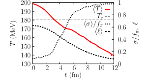
(b)

Figure 7: 7a Evolution of the average temperature, sigma field and Polyakov loop in a system evolving through the first order transition. Supercooling followed by reheating can be observed. The horizontal line denotes the critical temperature. 7b Evolution of the average temperature, sigma field and Polyakov loop in a system evolving through the CP. The temperature decreases monotonically with a small plateau slightly below $T_{c}$. The horizontal line denotes the critical temperature.

IV.4 Domain formation

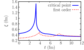
Figure 8: Correlation length of the sigma field as a function of time, for a CP and a first order transition scenario.

In our previous calculations we used the correlation functions (14) and (17) assuming that the stochastic noise fields in neighboring cells are not correlated as expressed by the spatial delta function. This leads to results that correspond to averaging over many events, see arXiv:1105.1962 . However, to better understand the differences between the two scenarios it is instructive to compare the microscopic structure of individual events. This requires a more consistent treatment of the field fluctuations by implementing realistic correlation lengths. Fig. 8 shows the correlation length of the sigma field $\xi=1/m_{\sigma}$ as a function of time for the expansion through both the CP and the first order phase transition. Here, $m_{\sigma}$ is calculated out of the volume averaged temperature in the previous section. The effect of such an averaging on the correlation length in inhomogeneous systems has been discussed in Nahrgang:2012qm . For the first order transition, $\xi$ lies in a range of $0.3-0.5$ fm for the whole evolution while in the CP scenario it reaches a peak of about $1.5$ fm when the system crosses the transition temperature after $t=3.2$ fm, cf. fig. 7b.

Below we present results obtained by correlating the noise fields over the spacelike distance $\xi=1/m_{\sigma}$ in each time step. The numerical procedure that implements such correlations has been described in Paech:2003fe . For each spatial cell we perform an averaging of the randomly distributed noise field over a surrounding cube of linear size $\xi=n\Delta x$ via

$$\xi_{\sigma}^{\prime}(\vec{x})=\frac{1}{n^{3}}\sum_{i,j,k=0,...,n-1}\xi_{\sigma}(\vec{x}+i\Delta x\vec{e}_{1}+j\Delta x\vec{e}_{2}+k\Delta x\vec{e}_{3})~{}.$$ (42)

As this procedure weakens the fluctuations, i. e. $\langle\delta\xi_{\sigma}^{\prime 2}\rangle\neq\langle\delta\xi_{\sigma}^{2}\rangle$, we have to rescale the noise field in order to obtain again the initial distribution width:

$$\xi_{\sigma}^{\prime\prime}(\vec{x})=\xi_{\sigma}^{\prime}(\vec{x})\sqrt{\frac{\langle\delta\xi_{\sigma}^{2}\rangle}{\langle\delta\xi_{\sigma}^{\prime 2}\rangle}}~{}.$$ (43)

An analogous correlation procedure is done for the Polyakov loop, correlating $\xi_{\ell}$ over the distance $1/m_{\ell}$. The following figures show spatial distributions in the transverse plane ($z=0$), for the sigma field in fig. 9, the Polyakov loop in fig. 10 and for the energy density in fig. 11. We chose a time of $t=4$ fm for the first order scenario corresponding to the onset of the transition process where $\langle T\rangle=T_{c}$, cf. fig. 7a. Here we expect to observe phase coexistence, i. e. domains of the chirally broken phase in the chirally symmetric background or vice versa. For the CP scenario we chose a time of $t=3.2$ fm, where again $\langle T\rangle=T_{c}$, cf. fig. 7b, and furthermore the correlation length reaches its maximum value as shown in fig. 8. In this scenario there are no degenerate or metastable phases around $T_{c}$ but one single equilibrium state for each temperature. We therefore expect a more regular structure with no domains.

By inspecting the figures we indeed find striking difference between the two transition scenarios. At the first order transition, both the fields and fluid evolve irregularly. This effect is best observed in the sigma field, fig. 9a, where one can see the expected domains of the chirally broken phase embedded in the chirally symmetric background, see for instance the region around $(x,y)=(2,2)$. Here, the system produces large fluctuations in small spatial regions that are able to overcome the potential barrier and create these characteristic structures. Nevertheless, the different phases are connected smoothly, there are no sharp boundaries between the domains. This is a result of the Laplacian in the equation of motion which smoothens the gradients. Also in the Polyakov loop, fig. 10a, and even more in the energy density, fig. 11a, we observe a bumpy and irregular structure. Regions of high energy density are embedded in a background of lower energy density in the periphery, like for instance around $(x,y)=(-2,5)$. These embedded regions are then going to grow and merge, leaving small islands of the symmetric phase which gradually shrink until the whole system is in the low temperature chirally broken phase.

On the other hand, the evolution through the CP proceeds smoothly, the regular ellipsoidal structure is preserved. Especially at the transition point, where the correlation length grows large, we see a smooth shape in both the fields and the energy density of the quark fluid, see figs. 9b, 10b and 11b. This striking difference in the event structure should manifest itself in the experimental data, e. g. in the non-statistical multiplicity fluctuations of produced hadrons Misshustin:2007jx .

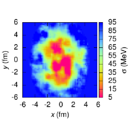
(a)

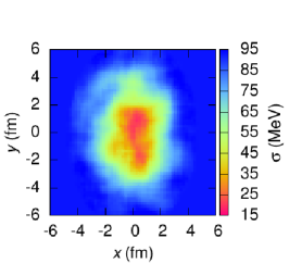
(b)

Figure 9: 9a Sigma field for $z=0$ at $t=4$ fm in a first order phase transition scenario. 9b Sigma field for $z=0$ at $t=3.2$ fm in a scenario with a CP.

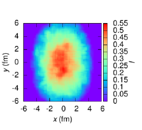
(a)

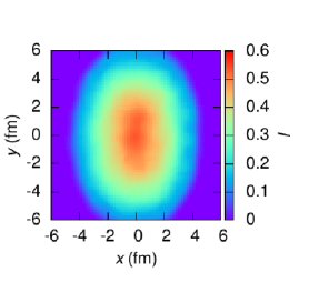
(b)

Figure 10: 10a Polyakov loop for $z=0$ at $t=4$ fm in a first order phase transition scenario. 10b Polyakov loop for $z=0$ at $t=3.2$ fm in a scenario with a CP.

(a)

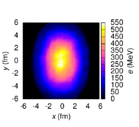
(b)

Figure 11: 11a Energy density for $z=0$ at $t=4$ fm in a first order phase transition scenario. 11b Energy density for $z=0$ at $t=3.2$ fm in a scenario with a CP.

V Summary and Outlook

We presented a fully dynamical model to study the chiral and deconfinement phase transitions of QCD simultaneously. In our previous studies of chiral fluid dynamics we have derived the coupled dynamics of the sigma field and the quark heat bath within a self-consistent 2PI effective action approach. The results were now extended for the Polyakov loop so that both order parameters are propagated via Langevin equations taking into account the interaction with the quark heat bath via dissipation and noise. We assume that the structure of the source term for the Polyakov loop is analogous to that for the sigma field. During all simulations the total energy is well conserved.

We studied the relaxational behavior of the coupled system for different quench scenarios in a box. For both the first order and the CP scenario, relaxation near the transition point is delayed. At the first order phase transition the relaxation process is significantly delayed due to the barrier in the thermodynamic potential. The transition actually starts only when this barrier disappears. Near the CP, when the sigma mass drops to zero and therefore the damping vanishes, we observe perpetual oscillations of the sigma field around the equilibrium value. These fluctuations are also visible in the Polyakov loop, although with a small amplitude. Performing a Fourier analysis of the fluctuations for both order parameter fields we have observed another interesting peculiarity. While during the transition process the intensity of fluctuations is much stronger in a first order than in a CP scenario, the soft modes are stronger enhanced near the CP as compared with the first order transition if the systems are allowed to equilibrate.

For the evolution of an expanding fluid through the first order transition we have found a clear evidence for the formation of a supercooled phase. Its decay later on leads to a substantial reheating of the quark fluid. That is in contrast to the simulation with a CP where the temperature decreases monotonically. Furthermore, during the onset of the first order transition, small domains of different phases coexist and create inhomogeneities in the energy density. In the CP scenario, where the correlation length grows large near the critical temperature, we observe a more homogeneous structure in the fields and fluid. A detailed analysis of domain formation at the first order phase transition will be provided in future work. Furthermore, we will extend this model to finite baryochemical potential and study trajectories in the full $T$-$\mu$-plane as well as fluctuations of baryon number densities.

We think about several extensions and refinements of the model. The damping coefficient for the sigma field should include not only the $\sigma\leftrightarrow q\bar{q}$ decay but also the decay into pions. The soft modes which are linked to the order parameter of the chiral transition are furthermore affected by interaction with the hard modes which would give another contribution to the heat bath and the dissipation process. For the Polyakov loop we used a purely phenomenological Langevin equation with a constant damping coefficient. This needs improvement, for instance by extracting this term from Monte Carlo simulations like it has been proposed in Fraga:2007gg . The present studies will allow for a better quantitative understanding of the signatures of the CP especially at FAIR energies.

References

- (1) Y. Aoki, G. Endrodi, Z. Fodor, S. D. Katz, K. K. Szabo, Nature 443 (2006) 675-678.
- (2) M. Cheng, N. H. Christ, S. Datta, J. van der Heide, C. Jung, F. Karsch, O. Kaczmarek and E. Laermann et al., Phys. Rev. D 74 (2006) 054507
- (3) Y. Aoki, Z. Fodor, S. D. Katz and K. K. Szabo, Phys. Lett. B 643 (2006) 46
- (4) Y. Aoki, S. Borsanyi, S. Durr, Z. Fodor, S. D. Katz, S. Krieg and K. K. Szabo, JHEP 0906 (2009) 088
- (5) S. Borsanyi et al. [Wuppertal-Budapest Collaboration], JHEP 1009 (2010) 073
- (6) O. Scavenius, A. Mocsy, I. N. Mishustin and D. H. Rischke, Phys. Rev. C 64 (2001) 045202.
- (7) B. -J. Schaefer and J. Wambach, Nucl. Phys. A757 (2005) 479
- (8) C. Ratti, M. A. Thaler, W. Weise, Phys. Rev. D 73 (2006) 014019.
- (9) B. -J. Schaefer, J. M. Pawlowski, J. Wambach, Phys. Rev. D 76 (2007) 074023.
- (10) V. Skokov, B. Friman and K. Redlich, Phys. Rev. C 83 (2011) 054904
- (11) V. Skokov, B. Friman, E. Nakano, K. Redlich and B. -J. Schaefer, Phys. Rev. D 82 (2010) 034029
- (12) B. -J. Schaefer, M. Wagner and J. Wambach, Phys. Rev. D 81 (2010) 074013
- (13) C. Sasaki and I. Mishustin, Phys. Rev. C 85 (2012) 025202
- (14) C. Sasaki, B. Friman and K. Redlich, Phys. Rev. D 77 (2008) 034024
- (15) M. A. Stephanov, K. Rajagopal and E. V. Shuryak, Phys. Rev. Lett. 81 (1998) 4816
- (16) M. A. Stephanov, K. Rajagopal and E. V. Shuryak, Phys. Rev. D 60 (1999) 114028
- (17) B. Berdnikov and K. Rajagopal, Phys. Rev. D 61 (2000) 105017
- (18) M. A. Stephanov, Phys. Rev. Lett. 102 (2009) 032301
- (19) F. Karsch and K. Redlich, Phys. Lett. B 695 (2011) 136
- (20) L. P. Csernai, J. I. Kapusta, Phys. Rev. D 46 (1992) 1379-1390.
- (21) L. P. Csernai and I. N. Mishustin, Phys. Rev. Lett. 74 (1995) 5005.
- (22) O. Scavenius, A. Dumitru, E. S. Fraga, J. T. Lenaghan and A. D. Jackson, Phys. Rev. D 63 (2001) 116003
- (23) J. Randrup, Phys. Rev. C 82 (2010) 034902.
- (24) J. Steinheimer and J. Randrup, [arXiv:1209.2462 [nucl-th]].
- (25) P. Chomaz, M. Colonna, J. Randrup, Phys. Rept. 389 (2004) 263-440.
- (26) I. N. Mishustin, Phys. Rev. Lett. 82 (1999) 4779
- (27) K. Rajagopal and F. Wilczek, Nucl. Phys. B404 (1993) 577
- (28) T. S. Biro and C. Greiner, Phys. Rev. Lett. 79 (1997) 3138
- (29) Z. Xu and C. Greiner, Phys. Rev. D 62 (2000) 036012
- (30) H. Caines [STAR Collaboration], [arXiv:0906.0305 [nucl-ex]].
- (31) A. Aduszkiewicz [NA61 Collaboration], Acta Phys. Polon. B 43 (2012) 635
- (32) B. Friman, C. Höhne, J. Knoll, S. Leupold, J. Randrup, R. Rapp, P. Senger (eds.), Lect. Notes Phys. 814 (2011) 1-980.
- (33) theor.jinr.ru/twiki-cgi/view/NICA/NICAWhitePaper
- (34) I. N. Mishustin and O. Scavenius, Phys. Rev. Lett. 83 (1999) 3134
- (35) K. Paech, H. Stoecker and A. Dumitru, Phys. Rev. C 68 (2003) 044907
- (36) M. Nahrgang, S. Leupold, C. Herold, M. Bleicher, Phys. Rev. C 84 (2011) 024912.
- (37) M. Nahrgang, S. Leupold and M. Bleicher, Phys. Lett. B 711 (2012) 109
- (38) M. Nahrgang, C. Herold, S. Leupold, I. Mishustin, M. Bleicher, [arXiv:1105.1962 [nucl-th]].
- (39) J. Peralta-Ramos and G. Krein, Phys. Rev. C 84 (2011) 044904
- (40) A. Dumitru and R. D. Pisarski, Phys. Lett. B 504 (2001) 282
- (41) A. Dumitru and R. D. Pisarski, Nucl. Phys. A698 (2002) 444
- (42) E. S. Fraga, G. Krein and A. J. Mizher, Phys. Rev. D 76 (2007) 034501
- (43) T. R. Miller and M. C. Ogilvie, Phys. Lett. B 488 (2000) 313
- (44) P. N. Meisinger, T. R. Miller and M. C. Ogilvie, Phys. Rev. D 65 (2002) 034009
- (45) R. D. Pisarski, Phys. Rev. D 62 (2000) 111501
- (46) C. Sasaki, B. Friman and K. Redlich, Phys. Rev. D 75 (2007) 074013
- (47) C. Ratti, S. Roessner and W. Weise, Phys. Lett. B 649 (2007) 57
- (48) S. Roessner, C. Ratti and W. Weise, Phys. Rev. D 75 (2007) 034007
- (49) C. Ratti and W. Weise, Phys. Rev. D 70 (2004) 054013
- (50) T. Heinzl, T. Kaestner and A. Wipf, Phys. Rev. D 72 (2005) 065005
- (51) P. de Forcrand and L. von Smekal, Phys. Rev. D 66 (2002) 011504
- (52) C. Wozar, T. Kaestner, A. Wipf, T. Heinzl and B. Pozsgay, Phys. Rev. D 74 (2006) 114501
- (53) T. K. Herbst, J. M. Pawlowski and B. -J. Schaefer, Phys. Lett. B 696 (2011) 58
- (54) K. Morita, V. Skokov, B. Friman and K. Redlich, [arXiv:1111.3446 [hep-ph]].
- (55) A. Mocsy, I. N. Mishustin and P. J. Ellis, Phys. Rev. C 70 (2004) 015204
- (56) M. Morikawa, Phys. Rev. D 33 (1986) 3607.
- (57) M. Gleiser and R. O. Ramos, Phys. Rev. D 50 (1994) 2441
- (58) D. Boyanovsky, I. D. Lawrie, D. S. Lee, Phys. Rev. D 54 (1996) 4013-4028.
- (59) C. Greiner and B. Muller, Phys. Rev. D 55 (1997) 1026
- (60) D. Bodeker, L. D. McLerran, A. V. Smilga, Phys. Rev. D 52 (1995) 4675-4690.
- (61) D. T. Son, [hep-ph/9707351].
- (62) D. H. Rischke, Phys. Rev. C 58 (1998) 2331
- (63) L. D. Landau, E. M. Lifschitz, “Lehrbuch der theoretischen Physik X: Physikalische Kinetik”, Akademie-Verlag Berlin (1983), p. 496
- (64) D. H. Rischke, S. Bernard, J. A. Maruhn, Nucl. Phys. A595 (1995) 346-382.
- (65) D. H. Rischke, Y. Pursun, J. A. Maruhn, Nucl. Phys. A595 (1995) 383-408.
- (66) N. C. Cassol-Seewald, R. L. S. Farias, E. S. Fraga, G. Krein and R. O. Ramos, [arXiv:0711.1866 [hep-ph]].
- (67) A. Abada and M. C. Birse, Phys. Rev. D 55 (1997) 6887 [hep-ph/9612231].
- (68) G. Amelino-Camelia, J. D. Bjorken and S. E. Larsson, Phys. Rev. D 56 (1997) 6942
- (69) M. Nahrgang, C. Herold, M. Bleicher, Quark Matter 2012 proceedings
- (70) I. N. Mishustin, PoS CPOD 07 (2007) 010