Abstract

The definition of order indices for density matrices is extended to finite systems. This makes it possible to characterize the level of ordering in such finite systems as macromolecules, nanoclusters, quantum dots, or trapped atoms. The general theory is exemplified by explicit calculations of the order index for the first-order density matrix of bosonic atoms confined in a finite box at zero temperature.

Keywords: Generalized density matrices, reduced density matrices, operator order indices, matrix order indices, trapped bosons

Corresponding Author:

V.I. Yukalov

Bogolubov Laboratory of Theoretical Physics

Joint Institute for Nuclear Research, Dubna 141980, Russia

E-mail: yukalov@theor.jinr.ru

Phone: +7(496) 21 63947 (office)

Fax: +7(496)21 65084

1 Introduction

We collaborated with John A. Coleman for 20 years, since 1990 till his death in 2010. Moreover, he was not merely our co-author, but during this time, he became our very close friend, with whom we spent many hours discussing various problems. We are keeping warmest memories of John and his wife Marie Jeanne. With great respect, we devote this paper to the memory of our friend and colleague John Coleman.

One of the interesting ideas, we developed with John Coleman, was the notion of the order indices for density matrices, introduced in Ref. [1]. The properties and applications of the order indices to different types of bulk matter, considered in thermodynamic limit, were studied in Refs. [2-5] and summarized in the book [6]. For infinite systems, however, it is possible to define the standard order parameters (see, e.g., [7,8]), because of which the use of the additional notion of the order indices could seem to be unnecessary. Nevertheless, as has been shown [1-3], the order indices are useful even for infinite systems, where a kind of mid-range order arises.

The principal difference of the order indices from the order parameters is that the former can be introduced not only for infinite systems, but also for finite systems. In recent years, the investigation of finite systems has become of high importance due to the widespread technological applications of various finite objects. As examples, we can mention quantum dots, metallic grains, different granular materials, nanoclusters, trapped atoms, and a variety of macromolecules, including biomolecules. For finite systems, as is well known, the order parameters are not defined [7,8]. In that case, the order indices can become principally important, as far as they can be defined for systems of any size. Then the order indices could characterize the amount of order specific for finite systems. It is the aim of the present paper to extend the definition and application of the order indices for finite systems.

In Sec. 2, we introduce the notion of order indices for arbitrary operators, which is specified for generalized density matrices in Sec. 3. The application to the usual reduced density matrices of statistical systems is given in Sec. 4, without invoking thermodynamic limit. In Sec. 5, we exemplify the consideration for bosonic atoms trapped in a finite box. Calculations for the order index of the first-order density matrix are given in Sec. 6, where the order index is treated as a function of the number of particles and of atomic interactions. Section 7 concludes.

2 Operator order indices

Order indices can be introduced for operators of any nature [9]. Let $\hat{A}$ be an operator acting on a Hilbert space $\mathcal{H}$. The operator is assumed to possess a norm $||\hat{A}||$ and a trace ${\rm Tr}\hat{A}$, with the trace taken over the space $\mathcal{H}$. In all other aspects, it can be arbitrary. The operator order index is

$$\omega(\hat{A})\equiv\frac{\log||\hat{A}||}{\log|{\rm Tr}\hat{A}|}\;.$$ (1)

The logarithm can be taken with respect to any base, since $\log_{a}z=\log_{b}z/\log_{b}a$. This definition connects the norm and trace of the operator through the relation

$$||\hat{A}||=|{\rm Tr}\hat{A}|^{\omega(\hat{A})}\;.$$ (2)

An operator $\hat{A}_{1}$ is said to be better ordered than $\hat{A}_{2}$, if and only if

$$\omega(\hat{A}_{1})>\omega(\hat{A}_{2})\;.$$ (3)

Respectively, two operators, $\hat{A}_{1}$ and $\hat{A}_{2}$ are equally ordered, provided that $\omega(\hat{A}_{1})=\omega(\hat{A}_{2})$.

The operator norm can be defined as a norm associated with the vector norm $|\varphi|$ for a nonzero vector $\varphi\in\mathcal{H}$, so that

$$||\hat{A}||=\sup_{\varphi}\;\frac{|\hat{A}\varphi|}{|\varphi|}\;.$$ (4)

Employing the scalar product $(\varphi,\varphi)$ for defining the norm yields the Hermitian vector norm $|\varphi|\equiv\sqrt{(\varphi,\varphi)}$. The corresponding Hermitian operator norm is

$$||\hat{A}||=\sup_{\varphi}\;\left[\frac{(\hat{A}\varphi,\hat{A}\varphi)}{(\varphi,\varphi)}\right]^{1/2}=\sup_{\varphi}\left[\frac{(\varphi,\hat{A}^{+}\hat{A}\varphi)}{(\varphi,\varphi)}\right]^{1/2}\;.$$ (5)

For an orthonormalized basis $\{\varphi_{k}\}$, labelled with an index $k$, in $\mathcal{H}$, such that

$${\cal H}={\rm Span}_{k}\{|\varphi_{k}\rangle\}\;,$$ (6)

the Hermitian norm (5) becomes

$$||\hat{A}||=\sup_{k}\left[(\hat{A}\varphi_{k},\hat{A}\varphi_{k})\right]^{1/2}\;.$$ (7)

If the operator $\hat{A}$ is self-adjoint, then its Hermitian norm simplifies to

$$||\hat{A}||=\sup_{\varphi}\;\frac{|(\varphi,\hat{A}\varphi)|}{|\varphi|}=\sup_{k}|(\varphi_{k},\hat{A}\varphi_{k})|\;.$$ (8)

The eigenfunctions of a self-adjoint operator, defined by the eigenproblem

$$\hat{A}\varphi_{k}=A_{k}\varphi_{k}\;,$$

form an orthogonal basis that can be normalized. The space basis can be chosen as the set of these eigenfunctions of the considered operator. Then the Hermitian norm becomes the spectral norm

$$||\hat{A}||=\sup_{k}|A_{k}|\;.$$ (9)

When the operator is semi-positive, then $|A_{k}|=A_{k}$.

For a semi-positive operator,

$$||\hat{A}||\leq{\rm Tr}\hat{A}\qquad(\hat{A}\geq 0)\;.$$

Therefore, for such an operator,

$$\omega(\hat{A})\leq 1\qquad(\hat{A}\geq 0)\;.$$ (10)

In that way, the order index (1) makes it possible to characterize the level of order in operators and to compare the operators as being more or less ordered. Instead of the Hermitian norm, one could employ some other types of operator norms, for instance, the trace norm [9]. But the use of the Hermitian norm is more convenient for physical and chemical applications.

3 Generalized density matrices

Self-adjoint operators play a special role in applications, defining the operators of observable quantities. One can resort to the coordinate representation, defining the physical coordinates through $x$, implying the set of all variables characterizing a particle. These can include Cartesian coordinates, spin, isospin, component-enumerating labels, and like that. The arithmetic space of all admissible values of the physical coordinates is denoted as ${\cal X}\equiv\{x\}$.

Let $\hat{\mathcal{A}}(x)$ be an operator of a local observable from the algebra of local observables ${\mathcal{A}}\equiv\{\hat{A}(x)\}$ given on the Fock space $\mathcal{F}$. And let ${\mathcal{A}}_{\psi}\equiv\{\hat{\psi}(x),\hat{\psi}^{\dagger}(x)\}$ be the algebra of field operators on $\mathcal{F}$, describing the system. The direct sum of these algebras is an extended local algebra

$${\cal A}_{ext}\equiv{\cal A}\bigoplus{\cal A}_{\psi}\;.$$ (11)

The set $x^{n}\equiv\{x_{1},x_{2},\ldots,x_{n}\}$ of the coordinates of $n$ particles pertains to the arithmetic space

$${\cal X}^{n}\equiv{\cal X}\times{\cal X}\times\ldots\times{\cal X}$$

that is an $n$-fold tensor product. The differential measure on the above space ${\mathcal{X}}^{n}$ is defined as

$$dx^{n}\equiv dx_{1}dx_{2}\ldots dx_{n}\;.$$

A function $\varphi(x^{n})$ can be treated as a vector

$$\varphi_{n}\equiv[\varphi(x^{n})]\in{\cal H}_{n}$$ (12)

in a Hilbert space ${\mathcal{H}}_{n}$, where the scalar product is given by

$$\varphi_{n}^{+}\varphi_{n}\equiv\int\varphi^{*}(x^{n})\varphi(x^{n})\;dx^{n}\;.$$ (13)

We consider a quantum system, whose state is given by a statistical operator $\hat{\rho}$ being a semi-positive self-adjoint operator normalized as

$${\rm Tr}_{\cal F}\hat{\rho}=1\qquad(\hat{\rho}^{+}=\hat{\rho}\geq 0)\;.$$ (14)

Taking any representative $A(x)$ of the extended algebra (11), we can define a matrix

$$\hat{D}_{A}^{n}\equiv\left[D_{A}(x^{n},y^{n})\right]\;,$$ (15)

which is a matrix with respect to the variables $x$, with the components

$$\hat{D}_{A}(x^{n},y^{n})\equiv{\rm Tr}_{\cal F}A(x_{1})\ldots A(x_{n})\hat{\rho}A^{+}(y_{n})\ldots A^{+}(y_{1})\;.$$ (16)

The action of matrix (15) on vector (12) is defined as the vector with the components

$$\hat{D}_{A}^{n}\varphi_{n}=\left[\int D_{A}(x^{n},y^{n})\varphi(y^{n})\;dy^{n}\right]\;.$$ (17)

As is seen from construction, matrix (15) is self-adjoint and semi-positive, because of which it can be termed the generalized density matrix.

The norm of matrix (15) is defined as

$$||\hat{D}_{A}^{n}||=\sup_{\varphi_{n}}\;\frac{\varphi_{n}^{+}\hat{D}_{A}^{n}\varphi_{n}}{\varphi_{n}^{+}\varphi_{n}}\;.$$ (18)

And the trace of this matrix is

$${\rm Tr}\hat{D}_{A}^{n}\equiv\int D_{A}(x^{n},x^{n})\;dx^{n}\;.$$ (19)

The order index of the generalized density matrix (15) is given by the expression

$$\omega(\hat{D}_{A}^{n})\equiv\frac{\log||\hat{D}_{A}^{n}||}{\log|{\rm Tr}\hat{D}_{A}^{n}|}\;,$$ (20)

with the norm and trace defined as above.

4 Reduced density matrices

A particular case of the generalized density matrices, being the most important for applications, is that of reduced density matrices. An $n$-th order reduced density matrix is the matrix

$$\hat{\rho}_{n}=[\rho(x^{n},y^{n})]\;,$$ (21)

with the components

$$\rho(x^{n},y^{n})\equiv{\rm Tr}_{\cal F}\hat{\psi}(x_{1})\ldots\hat{\psi}(x_{n})\hat{\rho}\hat{\psi}^{\dagger}(y_{n})\ldots\hat{\psi}^{\dagger}(y_{1})\;.$$ (22)

The relation of the reduced density matrix with the generalized density matrices is given by the equations

$$\hat{\rho}_{n}=\hat{D}_{\psi}^{n}\;,\qquad\rho(x^{n},y^{n})=D_{\psi}(x^{n},y^{n})\;.$$

Similarly to definition (20), the order index of the reduced density matrix (21) is

$$\omega(\hat{\rho}_{n})=\frac{\log||\hat{\rho}_{n}||}{\log{\rm Tr}\hat{\rho}_{n}}\;.$$ (23)

In this definition, we do not take thermodynamic limit, as in Refs. [1-3].

The eigenproblem

$$\hat{\rho}_{n}\varphi_{nk}=N_{nk}\varphi_{nk}$$ (24)

yields the eigenvalues

$$N_{nk}=\varphi_{nk}^{+}\hat{\rho}_{n}\varphi_{nk}$$ (25)

that define the spectral norm

$$||\hat{\rho}_{n}||=\sup_{k}N_{nk}\;.$$ (26)

And the trace of the $n$-th order density matrix is given [6] by the normalization

$${\rm Tr}\hat{\rho}_{n}=\frac{N!}{(N-n)!}\;.$$ (27)

We keep in mind a finite system with a finite number of particles $N$. This number is assumed to be sufficiently large, $N\gg 1$, but finite. For a large $N$ and fixed $n\ll N$, we can invoke the Stirling formula, yielding

$${\rm Tr}\hat{\rho}_{n}\simeq\left(\frac{N}{e}\right)^{n}\;.$$ (28)

Taking the natural logarithm gives

$$\ln{\rm Tr}\hat{\rho}_{n}=n(\ln N-1)\;.$$

Then the order index (23) reads as

$$\omega(\hat{\rho}_{n})=\frac{\ln||\hat{\rho}_{n}||}{n(\ln N-1)}\;.$$ (29)

From the properties of the reduced density matrices [6], we know that, in the case of Bose particles,

$$||\hat{\rho}_{n}||\leq(b_{n}N)^{n}\;,$$ (30)

where $b_{n}$ is a constant. This results in the inequality

$$\omega(\hat{\rho}_{n})\leq\frac{\ln N+\ln b_{n}}{\ln N-1}\qquad(Bose)\;.$$ (31)

For Fermi particles, depending on the order of the density matrices, we have

$$||\hat{\rho}_{2n-1}||\leq(c_{2n-1}N)^{n-1}\;,\qquad||\hat{\rho}_{2n}||\leq(c_{2n}N)^{n}\;,$$ (32)

because of which

$$\omega(\hat{\rho}_{2n-1})\leq\frac{(n-1)(\ln N+\ln c_{2n-1})}{(2n-1)(\ln N-1)}\;,$$

$$\omega(\hat{\rho}_{2n})\leq\frac{\ln N+\ln c_{2n}}{2(\ln N-1)}\qquad(Fermi)\;.$$ (33)

Taking into account large $N$ results in the inequalities for Bose particles,

$$\omega(\hat{\rho}_{n})\leq 1\qquad(Bose)\;,$$ (34)

and for Fermi particles,

$$\omega(\hat{\rho}_{2n-1})\leq\frac{n-1}{2n-1}\;,\qquad\omega(\hat{\rho}_{2n})\leq\frac{1}{2}\qquad(Fermi)\;.$$ (35)

5 Bose system with quasi-condensate

To give a feeling how the order indices describe physical ordering in finite systems, let us consider a cloud of $N$ Bose atoms trapped in a finite box of volume $V$. Systems of trapped Bose atoms are nowadays intensively studied both theoretically as well as experimentally [10-24]. We consider the case of either spinless atoms or that where atomic spins are frozen by an external magnetic field, so that the spin degrees of freedom are not important, but only the spatial variables $\bf r$ are considered.

As is known, in an infinite Bose system at low temperature, under thermodynamic limit, when $N\rightarrow\infty$, there appears Bose-Einstein condensate. But if the system is finite, no matter how large it is, there can be no well defined phase transition, hence, no Bose-Einstein condensation [20,24]. In a finite system, there can exist only a kind of quasi-condensate [25]. Below, we demonstrate the calculation of the order index for a Bose system in a finite box, at low temperature, when a quasi-condensate appears. For brevity, we shall often use the term condensate, keeping in mind quasi-condensate.

We start with the standard energy Hamiltonian

$$\hat{H}=\int\hat{\psi}^{\dagger}({\bf r})\left(-\;\frac{\nabla^{2}}{2m}\right)\hat{\psi}({\bf r})\;d{\bf r}\;+\;\frac{1}{2}\int\hat{\psi}^{\dagger}({\bf r})\hat{\psi}^{\dagger}({\bf r}^{\prime})\Phi({\bf r}-{\bf r}^{\prime})\hat{\psi}({\bf r}^{\prime})\hat{\psi}({\bf r})\;d{\bf r}d{\bf r}^{\prime}\;,$$ (36)

expressed through the field operators $\hat{\psi}(\bf r)$ satisfying the Bose commutation relations. Here and in what follows, the system of units is used, where the Planck and Boltzmann constants are set to one, $\hbar\equiv 1,k_{B}\equiv 1$.

To take into account the appearance of quasi-condensate, we employ the Bogolubov shift [26] of the field operator

$$\hat{\psi}({\bf r})=\eta({\bf r})+\psi_{1}({\bf r})\;,$$ (37)

separating it into the condensate function $\eta$ and the operator of the normal, uncondensed, particles $\psi_{1}$. To avoid double counting, the condensate and normal degrees of freedom are assumed to be orthogonal,

$$\int\eta^{*}({\bf r})\psi_{1}({\bf r})\;d{\bf r}=0\;.$$ (38)

The operator of uncondensed particles satisfies the conservation law

$$\langle\psi_{1}({\bf r})\rangle=0\;.$$ (39)

There are two normalization conditions, for the number of condensed particles,

$$N_{0}=\int|\eta({\bf r})|^{2}d{\bf r}\;,$$ (40)

and for the number of uncondensed particles,

$$N_{1}=\langle\hat{N}_{1}\rangle\;,$$ (41)

with the number operator of uncondensed atoms

$$\hat{N}_{1}\equiv\int\psi_{1}^{\dagger}({\bf r})\psi_{1}({\bf r})d{\bf r}\;.$$ (42)

The total number of atoms in the box is the sum

$$N=N_{0}+N_{1}\;.$$ (43)

To guarantee the validity of the normalization conditions (40) and (41), as well as the conservation law (39), it is necessary to introduce the grand Hamiltonian

$$H=\hat{H}-\mu_{0}N_{0}-\mu_{1}\hat{N}_{1}-\hat{\Lambda}\;,$$ (44)

in which

$$\hat{\Lambda}=\int\left[\lambda({\bf r})\psi_{1}^{\dagger}({\bf r})+\lambda^{*}({\bf r})\psi_{1}({\bf r})\right]d{\bf r}\;,$$ (45)

with $\mu_{0},\mu_{1}$, and $\lambda(\bf r)$ being the Lagrange multipliers.

The equations of motion are given by the variational equations for the condensate function

$$i\;\frac{\partial}{\partial t}\;\eta({\bf r},t)=\left\langle\frac{\delta H}{\delta\eta^{*}({\bf r},t)}\right\rangle$$ (46)

and for the field operator of uncondensed atoms

$$i\;\frac{\partial}{\partial t}\;\psi_{1}({\bf r},t)=\frac{\delta H}{\delta\psi_{1}^{\dagger}({\bf r},t)}\;,$$ (47)

where $t$ is time and the angle brackets imply statistical averaging. These equations are equivalent to the Heisenberg equations of motion [24,27].

The first-order reduced density matrix is

$$\rho({\bf r},{\bf r}^{\prime})=\langle\hat{\psi}^{\dagger}({\bf r}^{\prime})\hat{\psi}({\bf r})\rangle\;.$$ (48)

This, in view of the Bogolubov shift (37), reads as

$$\rho({\bf r},{\bf r}^{\prime})=\eta^{*}({\bf r}^{\prime})\eta({\bf r})+\langle\psi_{1}^{\dagger}({\bf r}^{\prime})\psi_{1}({\bf r})\rangle\;.$$ (49)

The eigenfunctions of the reduced density matrix (48) are called natural orbitals [6]. If these eigenfunctions are denoted as $\varphi_{k}(\bf r)$, with a labelling quantum multi-index $k$, then the spectrum of the density matrix is defined by the quantities

$$N_{1k}=\int\varphi_{k}^{*}({\bf r})\rho({\bf r},{\bf r}^{\prime})\varphi_{k}({\bf r}^{\prime})\;d{\bf r}d{\bf r}^{\prime}\;.$$ (50)

According to expression (49), there are two terms in the latter integral. One term,

$$N_{k}\equiv\left|\int\eta^{*}({\bf r})\varphi_{k}({\bf r})\;d{\bf r}\right|^{2}\;,$$ (51)

characterizes the condensed atoms, while another term,

$$n_{k}\equiv\int\varphi_{k}^{*}({\bf r})\langle\psi_{1}^{\dagger}({\bf r}^{\prime})\psi_{1}({\bf r})\rangle\varphi_{k}({\bf r}^{\prime})\;d{\bf r}d{\bf r}^{\prime}\;,$$ (52)

defines the distribution of uncondensed atoms. With the notation

$$a_{k}\equiv\int\varphi_{k}^{*}({\bf r})\psi_{1}({\bf r})\;d{\bf r}\;,$$ (53)

this distribution takes the form

$$n_{k}=\langle a_{k}^{\dagger}a_{k}\rangle\;.$$ (54)

In this way, the spectral norm of the density matrix (48) can be represented as

$$||\hat{\rho}_{1}||=\sup_{k}N_{1k}=\sup_{k}(N_{k}+n_{k})\;.$$ (55)

In a similar way, it is possible to find the norms of the higher-order density matrices. Thus, for the second-order density matrix, we would have to find out the pairon spectrum [28]. But here we concentrate on the properties of the first-order density matrix.

6 Order index behavior

Let us study the behavior of the order index

$$\omega(\hat{\rho}_{1})=\frac{\ln||\hat{\rho}_{1}||}{\ln N}$$ (56)

of the first-order density matrix (48). For atoms in a box of volume $V$, the natural orbitals are the plane waves

$$\varphi_{k}({\bf r})=\frac{1}{\sqrt{V}}\;e^{i{\bf k}\cdot{\bf r}}$$

labelled by the wave vector quantum number $k$. The condensate wave function reduces to a constant $\eta=\sqrt{N_{0}/V}$. Then the condensate spectrum (51) is

$$N_{k}=N_{0}\delta_{k0}\;.$$

The matrix eigenvalues (50) read as

$$N_{1k}=\delta_{k0}N_{0}+(1-\delta_{k0})n_{k}\;.$$ (57)

And norm (55) becomes

$$||\hat{\rho}_{1}||=\sup\{N_{0},\;\sup_{k}n_{k}\}\;.$$ (58)

To accomplish explicit calculations, we need to fix the form of the interaction potential entering Hamiltonian (36). We shall keep in mind dilute Bose gas for which the interaction potential is well modelled by the local form

$$\Phi({\bf r})=\Phi_{0}\delta({\bf r})\;,\qquad\Phi_{0}\equiv 4\pi\;\frac{a_{s}}{m}\;,$$ (59)

where $a_{s}$ is scattering length. We shall accomplish calculations invoking the Hartree-Fock-Bogolubov approximation in the self-consistent approach using representative ensembles [23,24,29].

We introduce the notations

$$\rho_{0}\equiv\frac{N_{0}}{V}\;,\qquad\rho_{1}\equiv\frac{N_{1}}{V}=\frac{1}{V}\sum_{k}n_{k}\;,$$

$$\rho\equiv\frac{N}{V}=\rho_{0}+\rho_{1}\;,\qquad\sigma_{1}=\frac{1}{V}\sum_{k}n_{k}\;,$$ (60)

defining the mean densities of condensed ($\rho_{0}$) and uncondensed ($\rho_{1}$) atoms, and also the so-called anomalous average $\sigma_{1}$, whose modulus $|\sigma_{1}|$ describes the number of correlated atomic pairs. The corresponding atomic distributions, at temperature $T$, read as

$$n_{k}=\frac{\omega_{k}}{2\varepsilon_{k}}\;\coth\left(\frac{\varepsilon_{k}}{2T}\right)-\;\frac{1}{2}\;,\qquad\sigma_{k}=-\;\frac{mc^{2}}{2\varepsilon_{k}}\;\coth\left(\frac{\varepsilon_{k}}{2T}\right)\;,$$ (61)

where

$$\omega_{k}\equiv mc^{2}+\frac{k^{2}}{2m}\;,\qquad\varepsilon_{k}\equiv\sqrt{(ck)^{2}+\left(\frac{k^{2}}{2m}\right)^{2}}\;.$$

The sound velocity $s$ satisfies the equation

$$mc^{2}=\Phi_{0}(\rho_{0}+\sigma_{1})\;.$$ (62)

Quasi-condensate can arise only at low temperature. For concreteness, we take zero temperature $T=0$. Then, from the above formulas, we have

$$n_{k}=\frac{\omega_{k}-\varepsilon_{k}}{2\varepsilon_{k}}\;,\qquad\sigma_{k}=-\;\frac{mc^{2}}{2\varepsilon_{k}}\;,$$

$$\rho_{1}=\frac{(mc)^{3}}{3\pi^{2}}\;,\qquad\sigma_{1}=\frac{(mc)^{2}}{\pi^{2}}\;\sqrt{m\rho_{0}\Phi_{0}}\;.$$ (63)

In the calculation of $\sigma_{1}$, we employ dimensional regularization [24,29].

It is convenient to introduce dimensionless quantities simplifying the formulas. Atomic interactions are characterized by the gas parameter

$$\gamma\equiv a_{s}\rho^{1/3}\;.$$ (64)

Dimensionless sound velocity is

$$s\equiv\frac{mc}{\rho^{1/3}}\;.$$ (65)

The condensate and anomalous fractions are

$$n_{0}\equiv\frac{N_{0}}{N}=\frac{\rho_{0}}{\rho}\;,\qquad\sigma\equiv\frac{\sigma_{1}}{\rho}\;.$$ (66)

In this dimensionless notation, the equation for the sound velocity (62) reduces to

$$s^{2}=4\pi\gamma(n_{0}+\sigma)\;,$$ (67)

the condensate fraction becomes

$$n_{0}=1-\;\frac{s^{3}}{3\pi^{2}}\;,$$ (68)

and the anomalous fraction is

$$\sigma=\frac{2s^{2}}{\pi}\;\sqrt{\frac{\gamma n_{0}}{\pi}}\;.$$ (69)

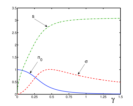
Figure 1: Dimensionless sound velocity $s$, quasi-condensate fraction $n_{0}$, and anomalous average $\sigma$ as functions of the gas parameter $\gamma$.

Numerical solution to these equations is shown in Fig. 1, where $s,\sigma$, and $n_{0}$ are presented as functions of the gas parameter (64).

The distribution of the normal atoms $n_{k}$ increases as $k$ diminishes. The minimal value of $k$ is prescribed by the box volume $V$, so that

$$k_{min}=\frac{1}{V^{1/3}}=\frac{\rho^{1/3}}{N^{1/3}}\;.$$ (70)

This gives

$$\sup_{k}n_{k}=\frac{s}{2}\;N^{1/3}\;.$$

Therefore, norm (58) is represented as

$$||\hat{\rho}_{1}||=\sup\left\{n_{0}N,\;\frac{s}{2}\;N^{1/3}\right\}\;.$$ (71)

The order index (56), for an infinite system in the presence of condensate, in thermodynamic limit $N\rightarrow\infty$, is exactly one, which corresponds to long-range order. But for a finite system, the order-index behavior is not so trivial, varying between zero and one, depending on the system parameters.

In the case of asymptotically weak atomic interactions, when $\gamma\rightarrow 0$, from Eqs. (67) to (69), it follows

$$n_{0}\simeq 1\;-\;\frac{8}{3\sqrt{\pi}}\;\gamma^{3/2}\;-\;\frac{64}{3\pi}\;\gamma^{3}\;,$$

$$\sigma\simeq\frac{8}{\sqrt{\pi}}\;\gamma^{3/2}+\frac{32}{\pi}\;\gamma^{3}\;,$$

$$s\simeq 2\sqrt{\pi}\;\gamma^{1/2}+\frac{16}{3}\;\gamma^{2}+\frac{32}{9\sqrt{\pi}}\;\gamma^{7/2}\;.$$ (72)

Then the matrix norm is

$$||\hat{\rho}_{1}||\simeq n_{0}N\qquad(\gamma\rightarrow 0)\;,$$

and the order index tends to

$$\omega(\hat{\rho}_{1})\simeq 1+\frac{\ln n_{0}}{\ln N}\;.$$

Using expansions (72), we find

$$\omega(\hat{\rho}_{1})\simeq 1-\;\frac{8\gamma^{3/2}}{3\sqrt{\pi}\ln N}\qquad(\gamma\rightarrow 0)\;.$$ (73)

As is seen, the order index reduces to one when either the interaction strength tends to zero or the system becomes infinite. But for a finite system of interacting atoms, the order index is less than one.

In the opposite case of arbitrarily strong interactions, when $\gamma\rightarrow\infty$, we have

$$n_{0}\simeq\frac{\pi}{64}\;\gamma^{-3}\;,$$

$$\sigma\simeq\frac{(9\pi)^{1/3}}{4}\;\gamma^{-1}\;-\;\frac{\pi}{64}\;\gamma^{-3}\;-\;\frac{1}{128}\left(\frac{\pi^{4}}{3}\right)^{1/3}\gamma^{-4}\;,$$

$$s\simeq\left(3\pi^{2}\right)^{1/3}\;-\;\frac{1}{64}\left(\frac{\pi^{5}}{9}\right)^{1/3}\gamma^{-3}\;.$$ (74)

For a finite system, with a fixed number of atoms $N$, when the interaction strength exceeds the value $0.317N^{2/9}$, we get

$$||\hat{\rho}_{1}||\simeq\frac{(3\pi^{2})^{1/3}}{2}\;N^{1/3}\qquad(\gamma\rightarrow\infty)\;.$$

Therefore, the order index behaves as

$$\omega(\hat{\rho}_{1})\simeq\frac{1}{3}+\frac{0.436}{\ln N}\qquad(\gamma\rightarrow\infty)\;,$$ (75)

which is again less than one.

Thus, we see that, for a finite system, the order index varies between unity, when the gas parameter tends to zero, and the limiting value (75), when the gas parameter tends to infinity. That is, a finite system can exhibit only a kind of quasi-long-range order, or mid-range order. The overall behavior of the order index (56) as a function of the interaction strength $\gamma$ and the number of atoms in the box $N$, is shown in Figs. 2 and 3. When $N$ tends to infinity, the order index tends to unity. In the scale of Fig. 3, this is not seen for $\gamma=1$, since $\omega(\hat{\rho}_{1})$ for this $\gamma$ decreases after $N=11$. In order to demonstrate that this is just a temporary decrease, we show the behavior of the order index $\omega(\hat{\rho}_{1})$, in a larger scale of $N$, in Fig. 4. As is seen, the order index diminishes till $N=200$, after which it increases. This increase is rather slow. Thus, for $N=10^{9}$, the order index reaches the value 0.9, and for $N=10^{80}$, it becomes 0.98. So that it tends to unity as $N\rightarrow\infty$.

7 Conclusion

The notion of order indices for reduced density matrices is extended to the case of finite systems. In such systems there can be no long-range order and the standard order parameters are not defined. Contrary to this, the order indices have the meaning for finite systems, characterizing the level of ordering in these objects. Examples of finite systems are quantum dots, metallic grains, nanoclusters, trapped atoms, and various macromolecules, including biomolecules.

Generally, in finite systems, there can exist only a kind of mid-range order. The level of such an order is well described by order indices. The suggested approach is illustrated by calculating the order index for the first-order reduced density matrix of bosonic atoms at zero temperature, trapped in a finite box. The order index, depending on the values of the number of atoms and the strength of their interactions, varies between zero and one.

The order indices can be defined for finite systems composed of several types of particles. For such a system of several components, it is possible to define the order index for the total system, as well as the partial order indices for some of the components. For example, it is often of interest the investigation of the properties of a particular kind of atoms entering a complex molecule [30]. Then the order indices can be introduced for the studied atoms characterizing the level of their ordering inside the molecule.

The order indices serve as a measure of internal ordering and correlations and could be used as an additional characteristic for finite quantum systems.

Acknowledgement

Financial support from the Russian Foundation for Basic Research is acknowledged.

Figure Captions

Fig. 1. Dimensionless sound velocity $s$, quasi-condensate fraction $n_{0}$, and anomalous average $\sigma$ as functions of the gas parameter $\gamma$.

Fig. 2. Order index $\omega(\hat{\rho}_{1})$ as a function of the gas parameter $\gamma$ for different number of atoms: $N=10$ (solid line), $N=10^{3}$ (dashed line), $N=10^{5}$ (dotted line), and $N=10^{7}$ (dashed-dotted line).

Fig. 3. Order index $\omega(\hat{\rho}_{1})$ as a function of the number of atoms for different gas parameters: $\gamma=0.001$ (upper solid line), $\gamma=0.1$ (dashed line), $\gamma=0.3$ (dotted line), $\gamma=0.5$ (dashed-dotted line), and $\gamma=1$ (lower solid line).

Fig. 4. Order index $\omega(\hat{\rho}_{1})$ for $\gamma=1$ as a function of the number of atoms $N$, demonstrating that this index increases as $N$ grows larger than 200. Numerical calculations show that the index tends to unity as $N\rightarrow\infty$.

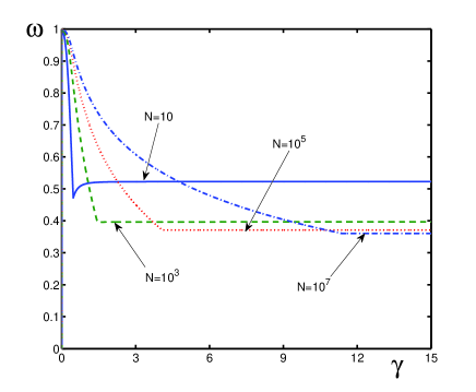
Figure 2: Order index $\omega(\hat{\rho}_{1})$ as a function of the gas parameter $\gamma$ for different number of atoms: $N=10$ (solid line), $N=10^{3}$ (dashed line), $N=10^{5}$ (dotted line), and $N=10^{7}$ (dashed-dotted line).

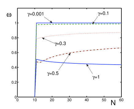
Figure 3: Order index $\omega(\hat{\rho}_{1})$ as a function of the number of atoms for different gas parameters: $\gamma=0.001$ (upper solid line), $\gamma=0.1$ (dashed line), $\gamma=0.3$ (dotted line), $\gamma=0.5$ (dashed-dotted line), and $\gamma=1$ (lower solid line).

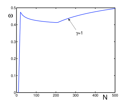
Figure 4: Order index $\omega(\hat{\rho}_{1})$ for $\gamma=1$ as a function of the number of atoms $N$, demonstrating that this index increases as $N$ grows larger than 200. Numerical calculations show that the index tends to unity as $N\rightarrow\infty$.

References

- [1] A.J. Coleman, V.I. Yukalov, Order indices and mid-range order, Mod. Phys. Lett. B 5 (1991) 1679–1686.
- [2] A.J. Coleman, V.I. Yukalov, Order indices for boson density matrices, Nuovo Cimento B 107 (1992) 535–552.
- [3] A.J. Coleman, V.I. Yukalov, Ordre indices and ordering in macroscopic systems, Nuovo Cimento B 108 (1993) 1377–1397.
- [4] A.J. Coleman, E.P. Yukalova, V.I. Yukalov, Superconductors with mesoscopic phase separation, Physica C 243 (1995) 76–92.
- [5] A.J. Coleman, V.I. Yukalov, Relation between microscopic and macroscopic characteristics of statistical systems, Int. J. Mod. Phys. B 10 (1996) 3505–3515.
- [6] A.J. Coleman, V.I. Yukalov, Reduced Density Matrices, Springer, Berlin, 2000.
- [7] L.D. Landau, E.M. Lifshitz, Statistical Physics, Pergamon, Oxford, 1980.
- [8] V.I. Yukalov, A.S. Shumovsky, Lectures on Phase Transitions, World Sientific, Singapore, 1990.
- [9] V.I. Yukalov, Matrix order indices in statistical mechanics, Physica A 310 (2002) 413–434.
- [10] L. Pitaevskii, S. Stringari, Bose-Einstein Condensation, Clarendon, Oxford, 2003.
- [11] E.H. Lieb, R. Seiringer, J.P. Solovej, J. Yngvason, The Mathematics of the Bose Gas and Its Condensation Birkhauser, Basel, 2005.
- [12] V. Letokhov, Laser Control of Atoms and Molecules, Oxford University, New York, 2007.
- [13] C.J. Pethik, H. Smith, Bose-Einstein Condensation in Dilute Gases, Cambridge University, Cambridge, 2008.
- [14] P.W. Courteille, V.S. Bagnato, V.I. Yukalov, Bose-Einstein condensation of trapped atomic gases, Laser Phys. 11 (2001) 659–800.
- [15] J.O. Andersen, Theory of the weakly interacting Bose gas, Rev. Mod. Phys. 76 (2004) 599–639.
- [16] V.I. Yukalov, Principal problems in Bose-Einstein condensation of dilute gases, Laser Phys. Lett. 1 (2004) 435–461.
- [17] K. Bongs, K. Sengstock, Physics with coherent matter waves, Rep. Prog. Phys. 67 (2004) 907–963.
- [18] V.I. Yukalov, M.D. Girardeau, Fermi-Bose mapping for one-dimensional Bose gases, Laser Phys. Lett. 2 (2005) 375–382.
- [19] A. Posazhennikova, Weakly interacting dilute Bose gases in 2D, Rev. Mod. Phys. 78 (2006) 1111–1134.
- [20] V.I. Yukalov, Bose-Einstein condensation and gauge symmetry breaking, Laser Phys. Lett. 4 (2007) 632–647.
- [21] N.P. Proukakis, B. Jackson, Finite-temperature models of Bose-Einstein condensation, J. Phys. B 41 (2008) 203002.
- [22] V.A. Yurovsky, M. Olshanii, D.S. Weiss, Collisions, correlations, and integrability in atom wave guides, Adv. At. Mol. Opt. Phys. 55 (2008) 61–138.
- [23] V.I. Yukalov, Cold bosons in optical lattices, Laser Phys. 19 (2009) 1–110.
- [24] V.I. Yukalov, Basics of Bose-Einstein condensation, Phys. Part. Nucl. 42 (2011) 460–513.
- [25] V.N. Popov, Functional Integrals in Quantum Field Theory and Statistical Physics, Reidel, Dordrecht, 1983.
- [26] N.N. Bogolubov, Lectures on Quantum Statistics, Gordon and Breach, New York, 1970, Vol. 2.
- [27] V.I. Yukalov Nonequilibrium representative ensembles for isolated quantum systems, Phys. Lett. A 375 (2011) 2797–2801.
- [28] A.J. Coleman, E.P. Yukalova, V.I. Yukalov, Pairon distributions and the spectra of reduced Hamiltonians, Int. J. Quant. Chem. 54 (1995) 211–222.
- [29] V.I. Yukalov, E.P. Yukalova, Bose-Einstein-condensed gases with arbitrary strong interactions, Phys. Rev. A 74 (2006) 063623.
- [30] D. Vanfleteren, D. Van Neck, P Bultinck, P.W. Ayers, M. Waroquier, Partitioning of the molecular density matrix over atoms and bonds, J. Chem. Phys. 132 (2010) 164111.