Distribution of Diffusion Constants and Stokes-Einstein Violation in supercooled liquids

Abstract

It is widely believed that the breakdown of the Stokes-Einstein (SE) relation between the translational diffusivity and the shear viscosity in supercooled liquids is due to the development of dynamic heterogeneity i.e. the presence of both slow and fast moving particles in the system. In this study we directly calculate the distribution of the diffusivity for a model system for different temperatures in the supercooled regime. We find that with decreasing temperature, the distribution evolves from Gaussian to bimodal indicating that on the time scale of the typical relaxation time, mobile (fluid like) and less mobile (solid like) particles in the system can be unambiguously identified. We also show that less mobile particles obey the Stokes-Einstein relation even in the supercooled regime and it is the mobile particles which show strong violation of the Stokes-Einstein relation in agreement with the previous studies on different model glass forming systems. Motivated by some of the recent studies where an ideal glass transition is proposed by randomly pinning some fraction of particles, we then studied the SE breakdown as a function of random pinning concentration in our model system. We showed that degree of SE breakdown increases quite dramatically with increasing pinning concentration, thereby providing a new way to unravel the puzzles of SE violation in supercooled liquids in greater details.

I Introduction

Dynamic heterogeneity (DH), which simply means multiple time scale relaxation processes in the system, is ubiquitous in all glass forming liquids and even in granular materials and gels. In many proposed theories of glass transition it is assumed without any explicit proof that there exists a broad distribution of relaxation times to explain many anomalous behaviours observed in supercooled liquids, e.g. breakdown of the Stokes-Einstein (SE) relation. In normal liquids, the shear viscosity is related to the translational diffusivity of a probe particle via the Stokes-Einstein relation SER08HM ; SER05Einstein ; SER87LL (discussed later). It has been shown extensively Th93HS ; SEB94KA ; SEB95TK ; SEB97CS ; SEB00EdigerReview ; SEB01MFCR ; SEB01ML ; 06KSD ; SEB06Chen ; SEB06BPS ; SEB09Xu ; SEB10M ; pap:LaNave-etal ; 12SKDS that when a liquid is supercooled, the measured self diffusivity becomes much larger than the value predicted by the SE relation. The shear viscosity is often substituted by the relaxation time which is roughly proportional to each other in the relevant temperature range (See ref.shiJCP2013 for an in-depth discussion on this issue). Phenomenological arguments Th93HS ; SEB95TK considering supercooled liquids to consist of mobile “fluid-like” and less mobile “solid-like” regions, can explain naturally the decoupling between the translational diffusion and the relaxation time. The average diffusivity is predominantly determined by the “fluid like” regions whereas the average relaxation time is dominated by the “solid-like” regions.

The existence of transient clusters of mobile and less mobile particles has been directly shown in many different studies DH-direct ; marcoMazza ; 09KDS ; 10KDSa . In 06KSD , distributions of displacements of particles were calculated for different densities for hard sphere fluid at different time intervals. It was shown that at large densities close to the glass transition density in this model, the distributions of displacements of particles show appearance of bimodality. A suitable cut off was then chosen to define the slow and fast particles in the system. They were also able to show that slow particles were largely obeying the SE relation over the whole density range studied and it is the fast particles which strongly violates the SE relation.

However, sometimes, e.g., in the phenomenological theories of SE breakdown, it is more natural to describe DH in terms of a distribution of diffusivity and relaxation times rather than displacements of particles. There are indirect evidences which support the existence of such a distribution - for example, the universal exponential tail in the Van Hove functions seen for many supercooled liquids 07CBK . Consider an extreme case where the system has regions with two diffusivity - one for “solid like” ($D_{1}$ ) and the other for “fluid like” regions ($D_{2}$). Hence a distribution of diffusivity can be written as $p(D,t)=A\delta(D-D_{1})+B\delta(D-D_{2})$ where $A$ and $B$ are fixed by the normalization condition and the amount of solid like and fluid like regions. Now if we calculate the van Hove correlation function as

$$G_{s}(x,t)=\int\,dD\,p(D,t)\,g(x|D,t),$$ (1)

where $g(x|D,t)=\frac{1}{\sqrt{4\pi Dt}}\exp{\left(-\frac{x^{2}}{4Dt}\right)}$, then one may show that the van Hove function will have a long tail and depending on the distribution of the $p(D,t)$, the tail of the distribution can be either exponential or Gaussian 12WKBG . In general the exponential tail has been reported 07CBK which, as mentioned in 12WKBG , might be due to the small range of data.

Now from the distribution of particle displacements one can calculate the distribution of diffusivity just by defining $D\sim\Delta r^{2}/\tau$, where $\Delta r^{2}$ is the square of the displacements of particles over some time interval $\tau$. However, we feel that the distribution of diffusivity calculated from the van Hove functions is more generic and robust. To substantiate our argument, lets take a system where diffusion process is anisotropic $\it e.g.$ diffusion along microtubule in biological context 12WKBG or diffusion of tagged particles in nematic liquids sDhara12 . Now on top of diffusion, if these molecules or tagged particles experience an internal drift force ($\it e.g.$ self propulsion) and one tries to calculate the diffusivity from the displacement, then the estimation of the diffusivity will be completely wrong. On the contrary, the method mentioned here will be free from these problems as the distribution of particle displacements along the anisotropic axis will have a non-zero mean value and one can easily decouple the over all drift of the system from the diffusion process and can still extract the distribution of the diffusivity without much difficulty. Although for isotropic systems both the methods will give the same results, the latter will be preferable in more general cases.

The key assumption in the method described here is that the long time dynamics of glass-forming liquids can be described by a superposition of diffusive processes. This is justified by the following argument: previous studies have shown that single particle trajectories in glass forming liquids can be described as short time vibrations inside cages with infrequent long time jumps due to cage breaking and formation of new cages. Thus, single-particle motion at long times and on a course grained length scale of a cage can be considered as diffusion among cages. We emphasize that particle displacements may be described by diffusive processes only for time intervals of the order of the time taken for the slope of the mean square displacement (MSD) to reach its asymptotic value 1, i.e. at least of the order of $\alpha$ relaxation times $\tau_{\alpha}$ (see Sec.III). Thus the distribution $P(D,t)$ is meaningful only for times greater than or equal to $\alpha$ relaxation times. We also note that the van Hove function is time dependent - having long time tail on the time scale of $\alpha$ relaxation times (when glass-forming liquids typically show maximum dynamical heterogeneity), but gradually becoming Gaussian in the limit of infinite time. Consequently the distribution of diffusivity must also be time dependent : $P(D,t)$ approaches a $\delta$ function asymptotically.

Our main aim in this study is to calculate directly this distribution of the diffusivity from the simulation data and thus understand the nature of DH. From the previous discussion, one may expect that in deeply supercooled liquids the distribution of diffusivity will be bimodal in general. Our results unambiguously show that the distribution of diffusivity indeed becomes bimodal below some temperature. However, the bimodal nature of the distribution does not prove that particles are clustered together to form “solid like” and “fluid-like” regions. Hence bimodality alone is not enough to justify the picture of supercooled liquids being a sparse mixture of “fluid like” and “solid like” regions. To test the existence of such clusters, we employ another kind of numerical experiment, where we probe the effect of random pinning on the system dynamics.

Recent studies 12KLP ; 13KP ; 03Kim ; 12BK ; 13KB ; cammarotaPinning ; 12CBEPL ; 13CGB ; 11KMS ; krakoviackPinning ; szamelPinning on dynamics of supercooled liquids in the presence of quenched disorder have shaded some interesting lights on the puzzles of glass transition including possible existence of ideal glass transition with increasing disorder strength cammarotaPinning . In most of the cases the quenched disorder is introduced by randomly freezing (pinning) some fraction of the particles in the system and it was found that relaxation time $\tau_{\alpha}$ increases drastically with increasing pinning concentration. The effect is so dramatic that in some simulation studies and subsequent mean-field and renormalization group analyses it was suggested that one can reach ideal glass state by simply increasing pinning fraction 12KLP ; 12BK ; cammarotaPinning . These studies have opened up a new avenue for exploring and understanding the puzzles of glass transition from a completely different perspective. One of the main findings of our study along these directions is the dramatic effect of random pinning on the SE break down. We show that the degree of SE breakdown can be very efficiently tuned by introducing random pinning in these model systems. Finally we argue from these observed effects of random pins that slow and fast particles indeed cluster to form “solid like” and “fluid like” regions in the system over the time scale of relaxation time, $\tau_{\alpha}$.

The paper is organised as follows : first we specify the simulation details and define the relevant quantities. Then we briefly explain the method used to extract the distribution of diffusivity and relaxation time. This methodology is then applied to a model supercooled liquid to understand the origin of dynamic heterogeneity and Stokes-Einstein breakdown. In the end we used random pinning geometry to further strengthen our conclusions reached from the analysis of distribution of diffusivity and relaxation time.

II Simulation Details

In the present study, we analyzed the Kob-Andersen binary mixture 95KA as a prototype glass-forming liquid. We performed NVT MD simulations using periodic boundary conditions at the constant number density $N/V=1.2$, where $N=1024$ was the system size and $V$ was the volume of the system. The units of length, energy and time were same as in Ref. 95KA . Integration time steps were $\delta t=0.005$ (in reduced units). At each state point, different quantities were averaged over $20$ different initial conditions, each run being at least 100 $\alpha$ relaxation times (defined in Sec. III) long.

III Definitions

van Hove function :

The van Hove function in one dimension is defined as $G(x,t)=\left\langle\frac{1}{N}\sum_{i=1}^{N}\sum_{j=1}^{N}\delta\left(x-x_{j}(t)+x_{i}(0)\right)\right\rangle$, where $x_{j}(t)$ is the $x$ coordinate of the position vector $\vec{r}_{j}(t)$ of the $j$th particle at time $t$ and $<.>$ implies averaging over time origins. In the present study, we compute the self part of the van Hove function (taking all particles) defined as

$$G_{s}(x,t)=\left\langle\frac{1}{N}\sum_{i=1}^{N}\delta\left(x-x_{i}(t)+x_{i}(0)\right)\right\rangle$$ (2)

Diffusivity ($D_{\infty}$) :

The mean squared displacement (MSD) is computed from $\left\langle\Delta r^{2}(t)\right\rangle=\left\langle\sum_{i=1}^{N}\left[\vec{r}_{i}(t)-\vec{r}_{i}(0)\right]^{2}\right\rangle$ (averaging over both the species). We denote the diffusivity computed from the long time limit of the MSD using the Einstein relation as $D_{\infty}$ :

$$\lim_{t\rightarrow\infty}\left\langle\Delta r^{2}(t)\right\rangle=6D_{\infty}t$$ (3)

Diffusivities for “solid-like” ($D_{s}$) and “fluid-like” ($D_{l}$) particles :

In the present study we identify subsets of particles as less mobile or “solid-like” or slow and more mobile or “fluid-like” or fast particles based on a distribution of diffusivity (see Sec I and IV for details). At low temperatures the distribution is multimodal and the peak positions are used for estimating “solid-like” and “fluid-like” diffusivities. At a given temperature, a “fluid-like” diffusivity $D_{l}$ is estimated from the positions of the peak at higher diffusivity. Similarly a “solid-like” diffusivity $D_{s}$ is estimated from the position of the peak at lower diffusivity. At the lowest three temperatures, where additional shoulders appear, the position of the dominant peak at lower diffusivity is taken to estimate $D_{s}$.

$\tau_{m}$, $\tau_{l}$ :

From the MSD, we compute two time scales $\tau_{m}$ and $\tau_{l}$ defined as the times when MSD at a given temperature respectively becomes 0.50 and 1.00 (in units of squared particle diameter $\sigma_{AA}^{2}$).

$$\left\langle\Delta r^{2}(\tau_{m})\right\rangle/\sigma^{2}_{AA}=0.50$$

$$\left\langle\Delta r^{2}(\tau_{l})\right\rangle/\sigma^{2}_{AA}=1.00$$ (4)

Relaxation time, $\tau_{\alpha}$ :

$\alpha$ relaxation times are computed from the decay of the overlap function. The overlap function $Q(t)$ is a normalized two point correlation function defined as 12SKDS

$$Q(t)=\left<\frac{1}{N}\sum_{i=1}^{N}w(|\vec{r}_{i}(t)-\vec{r}_{i}(0)|)\right>$$ (5)

with $w(x)=1.0$ for $x<0.30$ and zero otherwise. The summation is over all particles except for system with frozen particles, where the summation is only over the mobile particles and $N$ is the number of such particles. The $\langle\cdots\rangle$ indicates the averaging over time origin and different statistically independent simulation runs. Then $\tau_{\alpha}$ is defined as

$$Q(\tau_{\alpha})=1/e$$ (6)

Relaxation times for “solid-like” ($\tau_{s}$) and “fluid-like” ($\tau_{l}$) particles:

To calculate the $\alpha$ relaxation time of the “solid-like” or slow and “fluid-like” or fast particles, a suitable cut off is defined from the distribution of the diffusivity calculated at $\tau_{m}$. We choose the minimum of the distribution which appears at $D\tau_{m}\sim 0.060$ as the obvious cut off to define the slow and fast particles. A particle is defined to be slow if its squared displacement is less than or equal to $\Delta r^{2}=6D\tau_{m}\sim 0.360$ in time $t=\tau_{m}$, otherwise we define it as a fast particle. Once a set of slow and fast particles are defined for one time origin, we calculate the overlap function for slow $[Q_{s}(t)]$ and fast $[Q_{l}(t)]$ particles as

$$Q_{s}(t)=\left<\frac{1}{N_{s}}\sum_{i=1}^{N_{s}}w(|\vec{r}_{i}(t)-\vec{r}_{i}(0)|)\right>$$

$$Q_{l}(t)=\left<\frac{1}{N_{l}}\sum_{i=1}^{N_{l}}w(|\vec{r}_{i}(t)-\vec{r}_{i}(0)|)\right>,$$ (7)

where $N_{s}$ is the number of slow particles and $N_{l}=N-N_{s}$ is the number of fast particles. Notice that the number of slow and fast particles changes with different time origins and we then average all these correlation functions calculated at different time origins to get the average correlation function. The relaxation time $\tau_{s}$ or $\tau_{l}$ is then calculated as $Q_{s}(\tau_{s})=1/e$ and $Q_{l}(\tau_{l})=1/e$.

Stokes Einstein (SE) relation :

The Stokes Einstein relation connects the translational diffusivity $D_{B}$ of a probe Brownian particle inside a viscous liquid to the shear viscosity $\eta$ of the liquid : $D_{B}=c\frac{k_{B}T}{\eta}$, where $c$ is a constant whose value depends on the particle details and the boundary conditions and $T$ is temperature. In the present study, as often done in the literature, the diffusivity of the probe particle is replaced by the self diffusivity ($D_{\infty})$ of the liquid and the shear viscosity is replaced by the $\alpha$ relaxation time $\tau_{\alpha}$. Thus, we consider the following relation as the Stokes Einstein relation :

$$D_{\infty}=c\frac{k_{B}T}{\tau_{\alpha}}$$ (8)

SE violation parameters :

In many glass-forming liquids, the SE relation breaks down at low temperatures. The breakdown is characterized by a SE violation parameter $\theta(T)$ defined as :

$$\theta(T)=\frac{D_{\infty}\tau_{\alpha}}{T}$$ (9)

In addition, we compute SE violation parameters with the “solid-like” and “liquid-like” diffusivities as :

$$\theta_{s}(T)=\frac{D_{s}\tau_{s}}{T}$$

$$\theta_{l}(T)=\frac{D_{l}\tau_{l}}{T}.$$ (10)

Fractional SE relation and the breakdown exponent $w$ :

At low temperatures, where the SE relation $D_{\infty}\propto\tau_{\alpha}^{-1}$ breaks down, many glass-forming liquids obey a fractional SE relation SEB06BPS ; pap:SE-Douglas-Leporini :

$$D_{\infty}\propto\tau_{\alpha}^{-1+\omega}$$ (11)

where $\omega$ is denoted as the SE breakdown exponent. If $\omega=0$, the SE relation holds. In general, $0\leq\omega\leq 1$.

IV Distribution of Diffusivity

Lets start with briefly describing the method used to extract the distribution of diffusivity directly from the self van Hove correlation function $G_{s}(x,\tau)$ using the iterative algorithm suggested in 74Lucy and recently used in 12WKBG for diffusion processes in biological systems. We assume that particle displacements are caused by diffusion processes and there is a distribution of local diffusivity $p(D,\tau)$. Then we can express $G_{s}(x,\tau)$ in terms of $p(D,\tau)$ using Eq.1. Now given the $G_{s}(x,\tau)$, we calculate the distribution $p(D,\tau)$ following 74Lucy as

$$p^{n+1}(D,\tau)=p^{n}(D,\tau)\int_{-\infty}^{\infty}\frac{G_{s}(x,\tau)}{G^{n}_{s}(x,\tau)}g(x|D)dx,$$ (12)

where $p^{n}(D,\tau)$ is the estimate of $p(D,\tau)$ in the $n^{th}$ iteration with $p^{0}(D)=(1/D_{avg})\exp(-D/D_{avg})$ and

$$G^{n}_{s}(x,\tau)=\int_{0}^{D_{0}}\,p^{n}(D,\tau)\,g(x|D)\,dD.$$ (13)

We choose $D\tau$ as our variable because in the studied temperature range $D$ changes by several orders of magnitude whereas $D\tau$ changes relatively modestly. Hence

$$P^{n+1}(D\tau,\tau)=P^{n}(D\tau,\tau)\int_{-\infty}^{\infty}\frac{G_{s}(x,\tau)}{G^{n}_{s}(x,\tau)}g(x|D)dx,$$ (14)

where $p(D,\tau)dD=P(D\tau,\tau)d(D\tau)$.

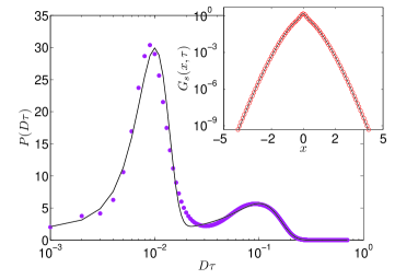
Figure 1: The solid line shows the results of the iterative scheme used to calculate the distribution of diffusivity (see text for details) along with the original distribution shown as symbols. The agreement is really encouraging and inset shows the corresponding comparison for the van Hove correlation functions.

We tested this iterative scheme first on a toy model to check its convergence. We started with a toy distribution defined as $P(x)\equiv A\exp\left[-(x-\mu_{1})^{2}/2\sigma_{1}^{2}\right]+B\exp\left[-(x-\mu_{2})^{2}/2\sigma_{2}^{2}\right]$ with the parameters $A,B,\mu_{1},\mu_{2},\sigma_{1},\sigma_{2}$ chosen by hand. Then we calculated the toy van Hove correlation function $G_{s}(x,\tau)$ using Eq.1, and used this as input to recalculate the probability distribution $P(D\tau)$ using Eq. 14. In Fig. 1, we have compared the calculated distribution $P(D\tau)$ with the exact distribution. The agreement is really good with moderate number of iterations. In the inset of Fig.1, we have compared the van Hove function obtained from the converged distribution of diffusivity with the exact one. Here also the agreement is near perfect. Note that the iterative scheme does not depend at all on the initial guess distribution as long as it is non-negative and normalizable.

V Distribution of Relaxation time

According to the criterion mentioned in the definition section, we first define slow and fast particles and then calculate their respective overlap correlation functions $Q_{s}(t)$ and $Q_{l}(t)$. The distribution functions are then calculated from these overlap functions using the following integral relation,

$$e^{-(t/\tau_{\alpha})^{\beta}}=\int_{0}^{\infty}e^{-t/\tau}P(\tau)d\tau.$$ (15)

where $\beta$ is the stretching parameter and also known as $KWW$ exponent in glass literature. Since the long time part of the overlap function $Q(t)$ can be very well described by stretched exponential form, one can try to extract the underlying distribution of relaxation time $P(\tau)$ by inverting the above equation. Analytical solution for this method is not directly available but some work along this line in alvarez provides some useful insights and highlights difficulties associated with this problem. Here we have extracted this distribution within the Gaussian approximation by optimizing the following cost function

$$\chi^{2}=\frac{1}{n}\sum_{i=1}^{n}\left[Q_{\nu}(t_{i})-\int_{0}^{\infty}e^{-t_{i}/\tau}P(\tau)d\tau\right]^{2}$$ (16)

with respect to the parameters of the $P(\tau)$. $\nu$ denotes slow (s) or fast (l) particles index. We choose the following functional form for $P(\tau)$

$$P(\tau)=\frac{1}{\tau\sqrt{2\pi}\sigma}e^{-\frac{(\log(\tau)-\log(\tau_{0}))^{2}}{2\sigma^{2}}}$$ (17)

such that $\int_{0}^{\infty}P(\tau)d\tau=1.0$. This is partly motivated by Ref.alvarez , where the formal expression of the distribution is written in terms of logarithm of the variable. So within Gaussian approximation, it becomes log-normal in $\tau$.

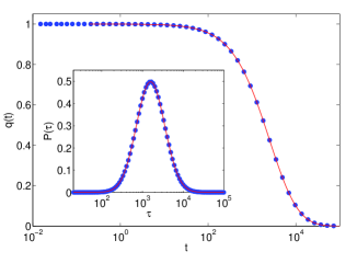
Figure 2: Plot of the stretched exponential function $q(t)$ (filled circles) as a function of time and the line is the corresponding output from the optimization of cost function in Eq.16. Inset: the comparison of the distribution of $\tau$ (filled circle) with the solution obtained from the optimization procedure (see text for details). The convergence of this optimization is very quick and does not depend on the initial parameter value.

To check the convergence of this method to the correct solution, we first tested it on a toy problem where we have generated a stretched exponential function $q(t)$ by using Eq.15 with a set of chosen values of $\tau_{0}$ and $\sigma$ and then performed the optimization of the cost function in Eq.16. In Fig.2, we show the convergence of this optimization procedure for the toy function. The convergence is quick and does not depend on the initial guess values of the parameters, $\tau_{0}$ and $\sigma$. In the result section we then use this optimization procedure to extract the distribution of relaxation time associated with the slow and fast particles i.e. $P(\tau_{s})$ and $P(\tau_{l})$ (see Results section for further details).

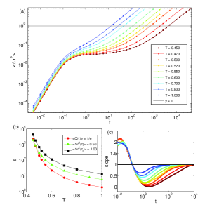
Figure 3: (a) Mean Squared displacement (MSD) for different temperature with the horizontal line indicating the time where mean squared displacement reaches $1.00$ in reduced units for different temperatures. The corresponding time is denoted as $\tau_{l}$ here. Correspondingly $\tau_{m}$ is defined as the time where the MSD goes to $0.50$ in reduced units. (b) Comparison of the $\alpha$-relaxation time $\tau_{\alpha}$ with $\tau_{m}$ and $\tau_{l}$ (see text for definitions). (c) Time dependence of the slope $\frac{d\ln<\Delta r^{2}(t)>}{d\ln t}$ of the MSD at different temperatures.

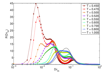
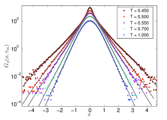
Figure 4: Calculated distribution of diffusivity at times $\tau_{m}$ for different temperatures. Notice the appearance of the bimodality in the distribution just below the onset temperature $T=1.00$. Clear bimodal distribution in the supercooled regime confirms that there are two different types of particles in terms of their mobility up to time scales of typical relaxation times. The appearance of more peaks in the distribution at still further lower temperature is really interesting, indicating possibility of extremely slow to moderately slow to very fast particles in very deep supercooled state.

Figure 5: The van Hove correlation functions at times $\tau_{m}$ (solid line) as obtained from the iterative scheme (see text for details) along with the simulation data (symbols). The curves are shifted upward for clarity and to point out that the line goes though the data points over the whole range of the data.

VI Results

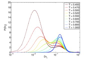
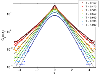
Figure 6: Top: The distribution of diffusivity at times $\tau_{l}$ for different temperatures. Even at $\tau_{l}$, the distribution is unimodal at high temperatures and bimodal at low temperatures. Bottom : Comparison of the van hove functions at times $\tau_{l}$ at different temperatures, computed from the diffusivity distribution (solid lines) and directly measured (symbols).

After establishing the rapid convergence of the iterative scheme we tried to calculate the distribution of diffusivity for a model glass forming liquid, the Kob-Andersen binary mixture 95KA . We calculated the self van Hove functions at different temperatures for the times $\tau_{m}$ and $\tau_{l}$ when the mean square displacement (MSD) [see panel (a) of Fig.3] becomes half and one respectively in reduced units. In the panel (b) of Fig.3, we have shown the temperature dependence of these different time scales. It is important to mention that $\tau_{l}$ is roughly the time where the logarithmic time derivative of MSD with time $\frac{d\ln\left\langle\Delta r^{2}(t)\right\rangle}{d\ln t}$ becomes very close to $1.0$ [see panel (c) of Fig.3]. This is the time when the underlying relaxation process can be well approximated by diffusion. We have repeated our calculation at two different time scales just to make sure that the outcome is not an artifact of doing the calculation at somewhat shorter time scale $\tau_{m}$ close to $\alpha$ relaxation times $\tau_{\alpha}$. Although $\tau_{m}$ is of the order of $\tau_{\alpha}$, the temperature dependence of $\tau_{m}$ is different from that of the $\alpha$-relaxation time $\tau_{\alpha}$.

At this point we would like to justify our choice of using $\tau_{m}$ (or $\tau_{l}$ ) for analysis. We wanted to compare a quantity (self van Hove function) which is a function of displacement across different temperatures and a natural choice is to have the mean squared displacement for these different temperatures to be same. We can also take a fixed time (say structural relaxation time or some multiple of it) and then compare the function but our guess is that the qualitative result will not change much. The temperature where the distribution of diffusivity calculated from self van Hove function starts to show bimodality (discussed later) may change a bit depending on this choice.

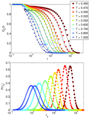
Figure 7: Top Panel: Overlap correlation function $Q_{s}(t)$ for the slow particles for different temperatures (filled symbols) and the lines are the corresponding best fit stretched exponential function obtained by optimizing Eq.16 with the corresponding best estimation of the distribution functions ( bottom panel).

To extract the distribution functions of diffusivity one needs to supply somewhat smoothly averaged data of the van Hove functions for the iterative scheme to converge rapidly. We fitted the extreme tails of the calculated van Hove functions using exponential functions as the tails are in general noisy and difficult to average. We have shown the distributions $P(D\tau_{m},\tau_{m})$ for different temperatures in Fig.5 and the van Hove functions calculated from these distributions along with the simulation data in Fig.5. The agreement between the simulation data and the calculated ones is indeed very good. Notice that tails of these van Hove functions can not be completely described by a single exponential function over the whole range at least for the low temperature data ($T\leq 0.50$). Rather they are better fitted by two exponential functions. Similar analysis at a later time $\tau_{l}$ shows no qualitative change in our results (Fig.6). Note that these results do not change with different dynamics e.g. Brownian dynamics, as MSD from molecular dynamics and from Brwonian dynamics become identical at time scales of the order of $\tau_{\alpha}$.

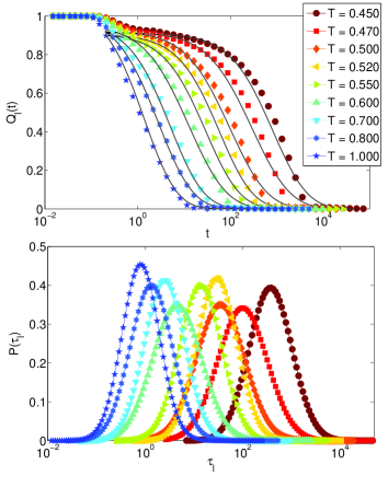
Figure 8: Top Panel: Overlap correlation function $Q_{l}(t)$ for the fast particles for different temperatures (filled symbols) and the lines are the corresponding best fit stretched exponential function obtained by optimizing Eq.16 with the corresponding best estimation of the distribution functions ( bottom panel).

Now looking at Fig.5, we can see that just below the onset temperature ($T=1.00$), the distribution starts to become bimodal and two peaks clearly emerge at temperature around $T=0.60$. At further lower temperatures the distributions seem to show existence of shoulders or another peak but the peak at large diffusivity remains intact with decreasing peak height. Thus we have clearly demonstrated that there are two types of particles in the supercooled liquid on the time scale of the order of $\tau_{\alpha}$. Notice that the width of the distribution increases with decreasing temperature which indicates increase of DH leading to stronger SE breakdown 12SKDS .

We have calculated the distribution of the relaxation times $\tau_{l}$ and $\tau_{s}$ using the optimization procedure described in Sec.V from the respective overlap correlation functions $Q_{l}(t)$ and $Q_{s}(t)$. We used data for $Q_{s}(t)$ or $Q_{l}(t)$ in range $0<Q_{s}(t)<0.85$ and $0<Q_{l}(t)<0.85$ for the optimization as short time part of the overlap function can not be represented by stretched exponential form. In top panel of Fig.7 we have shown the overlap correlation function for the slow particles for different temperatures and the corresponding best fit stretched exponential functions obtained by optimizing the cost function in Eq.16 with respect to the parameters of the distribution function $P(\tau_{s})$. The optimized distributions themselves are shown in bottom panel of Fig.7. One can see that stretched exponential function obtained are quite good fit to the $Q_{s}(t)$ data at higher temperature and seems to become little bad at lower temperature but overall it is quite good. It will be nice to be able to extract this distribution without the Gaussian approximation and work along this line is in progress. At this point we would like to point out that distribution of relaxation time calculated in PH99 is essentially same as that of the distribution of the diffusivity as it was calculated by estimating the time taken by individual particles to move a certain distance and this time is nothing but diffusion time. In Fig.8, we showed the results of similar analyses done for the fast particles.

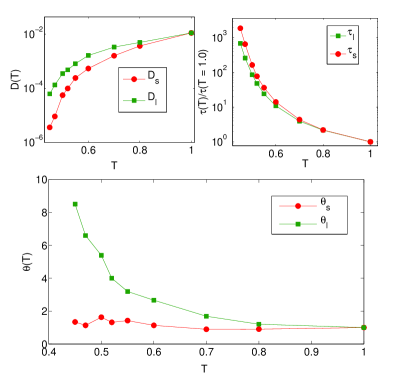
Figure 9: Top left panel: The temperature dependence of the diffusivity associated with the solid like ($D_{s}$) and fluid like ($D_{l}$) particles. These values are calculated from the peak positions of the distributions in Fig.5. Top right panel: The temperature dependence of the relaxation times of slow ($\tau_{s}$) and fast ($\tau_{l}$) particles (see text for definitions). Bottom panel: The Stokes-Einstein violation parameters $\theta_{s}(T)=D_{s}\tau_{s}/T$ (circle) and $\theta_{l}(T)=D_{l}\tau_{l}/T$ (square) for the two types of particles. One sees clearly that solid like particles obey Stokes-Einstein relation to a reasonable accuracy over the whole temperature range and it is the fluid like particles which show strong Stokes-Einstein violation.

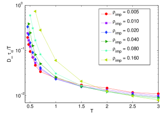
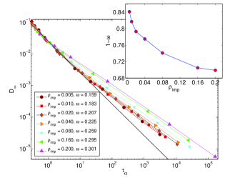
Figure 10: Left Panel: Stokes-Einstein violation parameter $\theta(T)$ has been shown as a function of temperature for different density of the frozen particles $\rho_{imp}$. One can clearly see that the deviation from the Stokes-Einstein relation becomes stronger with increasing density of the frozen particles. Right Panel: Diffusivity ($D_{\infty}$) plotted as a function of relaxation time ($\tau_{\alpha}$) for different density of the frozen particles $\rho_{imp}$ in log-log to show the power law relationship between these quantities expected from the fractional Stokes-Einstein Relation $D_{\infty}\propto\tau_{\alpha}^{-1+\omega}$, with $\omega\geq 0$. Notice that the exponent $\omega$ increase with increasing pinning density $\rho_{imp}$ indicating a stronger breakdown of the Stokes-Einstein Relation. The solid line has a slope equal to $-1.0$. Inset: The SE breakdown exponent as a function of $\rho_{imp}$.

After obtaining the distribution of diffusivity and relaxation times for the slow and fast particles respectively, we now try to understand the SE breakdown for both slow and fast particles separately. In top left panel of Fig.9, we have shown the temperature dependence of diffusivities associated with the solid like ($D_{s}$) and the fluid like ($D_{l}$) particles (defined in Sec. III). The corresponding time scales $\tau_{s}$ and $\tau_{l}$ are shown in the right panel of the same figure. In the bottom panel of Fig.9, we calculated the Stokes-Einstein violation parameters $\theta_{s}(T)=D_{s}\tau_{s}/T$ and $\theta_{l}(T)=D_{l}\tau_{l}/T$ for the two sets of particles. One clearly sees that solid like particles obey the Stokes-Einstein relation over the whole temperature range, whereas the fluid like particles show strong SE violation leading to overall violation of the SE relation in the liquid.

Note that in general one can think of the following scenarios which can lead to the SE breakdown in supercooled liquids:

1. Both slow and fast particles violate the SE relation simultaneously SEB06BPS .

2. Slow particles obey the SE relation and fast particles lead to violation.

3. Both slow and fast particles obey SE relation separately but the combined effect leads to SE violation when one considers average relaxation time and the bulk diffusion coefficient.

4. Slow particles violate but fast particles obey the SE relation.

So in this work we are able to rule out some of these possibilities and show that the SE break down is caused by the fast moving particles only. It should also be noted that we have defined slow and fast particles using some cut off parameter and the distributions are calculated based on this definition. Although the cut off parameter chosen in this work is not completely adhoc, the results might depend on the specific choice of this parameter. We believe that results will be fairly insensitive to small variation in the value of the cut off parameter and conclusion reached on the cause of the SE breakdown will be same over that range. Thus a method to determine the distribution of local relaxation times without invoking any arbitrary cut off parameter will be very much desirable to remove all these ambiguities in understanding the SE breakdown in supercooled liquids.

After identifying two types of particles in the system on the time scale of $\alpha$ relaxation time, we now turn to the question of whether the “solid-like” particles form clusters. To answer this, we performed simulations with some fraction $\rho_{imp}$ of the particles randomly frozen in space and time and studied the effect of this protocol on the dynamics of the system 12KLP ; 13KP ; 03Kim ; 12BK ; 13KB ; 11KMS . If the “solid like” particles form clusters then if we randomly freeze some particles, there will always be instances where these frozen particles are part of the “solid like” regions. In that case, due to the frozen particles, the relaxation of these regions will be hindered further and the relaxation time of the whole system will increase dramatically with increasing density of these frozen particles. However, these frozen particles will have very little effect on diffusivity which is mainly governed by the “fluid like” particles, so the diffusivity will not change dramatically. In this scenario, we expect to see an enhancement of the Stokes-Einstein breakdown with increasing $\rho_{imp}$. On the contrary if “solid-like” particles do not form clusters, then we expect that increasing $\rho_{imp}$ will have little effect on the relaxation dynamics of these regions i.e. no enhancement of the SE breakdown with $\rho_{imp}$. In the left panel of Fig.10, the temperature dependence of the SE violation parameter $\theta(T)=D_{\infty}\tau_{\alpha}/T$ for different pinning densities $\rho_{imp}$ shows dramatic deviation of $\theta(T)$ from constancy with increasing $\rho_{imp}$. Equivalently, by representing our data in $D_{\infty}$ vs. $\tau_{\alpha}$ (log-log) plot in the right panel of Fig.10, we see that in the low temperature range the system obeys a fractional Stokes-Einstein relation $D\propto\tau_{\alpha}^{-1+\omega}$, with $\omega\geq 0$, where the SE breakdown exponent $\omega$ increases significantly with increasing $\rho_{imp}$. In the past, many people have tried to tune the Stokes-Einstein breakdown exponent to better understand the physics behind it, either by tuning interaction potentials pap:SE-Affouard2009 or by changing spatial dimensions DIM09ER ; DIM10CIMM ; DIM12CPZ as one expects mean field results of $\omega=0$ to be exact at very large spatial dimension. Our results provides yet another way of tuning the SE breakdown exponent $\omega$ which we feel will have interesting implications on the possible existence of ideal glass transition with increasing pinning concentration as predicted in cammarotaPinning .

VII Conclusions

To conclude, (a) we have directly calculated the distributions of diffusivity for different temperatures for a model glass former in the supercooled regime. This unambiguously shows that the state of the system can be well described by a mixture of “fluid like” and “solid like” particles on the time scale of $\alpha$ relaxation time. This enabled us to extract the distributions of relaxation times for slow and fast particles and helped us to discover that only fast particles are responsible for the Stokes-Einstein breakdown in bulk supercooled liquids; (b) we demonstrate, using a procedure (random pinning) which does not involve any arbitrary cut-off, that the “solid-like” particles form clusters on the time scale of $\alpha$ relaxation time; and (c) finally we show that random pinning can drastically enhance the decoupling between the translational diffusion and the relaxation time, thereby providing a new and easy way to tune the SE breakdown exponent.

The last result we believe is very significant in understanding the origin of the SE breakdown in supercooled liquids. In DIM12CPZ , it is conjectured that local hopping, facilitation and dynamical heterogeneity together play significant roles in SE breakdown and the contribution of dynamic heterogeneity might become smaller with increasing dimensionality but how other contributions changes with dimensionality is not very clear. Now random pinning might help us to resolve this issue. For example it will be useful to understand whether the increase in the SE breakdown exponent $\omega$ is related to the increase in dynamic heterogeneity in the random pinning case also. It will also be important to study the SE breakdown by simultaneously changing both dimensionality and fraction of randomly pinned particles to pin point the correct reason behind the SE breakdown. Finally it will be interesting to also extract the length scale associated with the “solid like” and “fluid like” regions and compare that with the dynamic heterogeneity length scale 09KDS and the static length scales 12KLP ; SauTar10 ; BeKo_PS ; HocRei12 ; 12KP ; 08BBCGV ; 13BKP .

We would like to thank Srikanth Sastry, Chandan Dasgupta and Saurish Chakrabarty for many useful discussions.

References

- (1) J. HANSEN and I. R. MCdONALD, Theory of Simple Liquids (3rd Ed.), Elsevier (2008).
- (2) A. EINSTEIN, Ann. Phys. 17, 549 (1905); English translation: A. EINSTEIN, Investigations on the theory of the Brownian movement, Dover, NY (1956).
- (3) L. D. LANDAU and E. M. LIFSHITZ, Fluid Mechanics, 2nd. Ed., Pergamon Press (1987).
- (4) J. A. HODGDON and F. H. STILLINGER, Phys. Rev. E, 48, 207 (1993); F. H. STILLINGER and J. A. HODGDON, Phys. Rev. E, 50, 2064 (1994).
- (5) W. KOB and H. C. ANDERSEN, Phys. Rev. Lett., 73, 1376 (1994).
- (6) G. TARJUS and D. KIVELSON, J. Chem. Phys., 103, 3071 (1995).
- (7) I. CHANG and H. SILESCU, J. Phys. Chem. B, 101, 8794 (1997).
- (8) M. D. EDIGER, Annu. Rev. Phys. Chem. 51, 99 (2000).
- (9) C. DE MICHELE and D. LEPORINI, Phys. Rev. E 63 036701 (2001).
- (10) G. MONACO, D. FIORETTO, L. COMEZ and G. RUOCCO, Phys. Rev. E, 63, 061502, (2001).
- (11) S. KUMAR, G. SZAMEL and J.F. DOUGLAS J. Chem. Phys. 124, 214501 (2006).
- (12) S. CHEN et al., Proc. Natl. Acad. Sci. (US), 103, 12974 (2006).
- (13) S. BECKER, P. POOLE, F. STARR, Phys. Rev. Lett., 97, 055901, (2006).
- (14) E. LA NAVE, S. SASTRY and F. SCIORTINO, Phys. Rev. E, 74, 050501(R) (2006).
- (15) L. XU et al., Nature Physics, 5, 565, (2009).
- (16) F. MALLAMACE et al., J. Phys. Chem. B, 114, 1870, (2010).
- (17) S. SENGUPTA, S.KARMAKAR, C. DASGUPTA and S. SASTRY, J. Chem. Phys., 138, 12A548 (2013).
- (18) Z. SHI, P. G. DEBENEDETTI, and F. H. STILLINGER, J. Chem. Phys. 138, 12A526 (2013).
- (19) W. K. KEGEL and A. VAN BLAADEREN, Science, 287, 290 (2000); E. R. WEEKS, J.C. CROCKER, A. C. LEVITT, A. SCHOELD and D.A. WEITZ, Science, 287, 627 (2000); A. WIDMER-COOPER, H. PERRY, P. HARROWELL and D. R. REICHMAN, Nat. Phys., 4, 711, (2008).
- (20) M.G. MAZZA, N. GIOVAMBATTISTA, FW. STARR, HE. STANLEY, Phys. Rev. Lett. 96, 057803 (2006).
- (21) S. KARMAKAR, C. DASGUPTA, and S. SASTRY, Proc. Nat. Acad. Sci. (USA) 106, 3675 (2009).
- (22) S. KARMAKAR, C. DASGUPTA, and S. SASTRY, Phys. Rev. Lett. 105, 015701 (2010).
- (23) P. CHAUDHURI, L. BERTHIER and W. KOB , Phys. Rev. Lett. 99, 060604 (2007).
- (24) B. WANG, J. KUO, S.C. BAE and S. GRANICK, Nat. Mat. 11, 481 ( 2012 ).
- (25) S. DHARA, Y. BALAJI, J. ANANTHAIAH, P. SATHYANARAYANA, V. ASHOKA, A. SPADLO, and R. DABROWSKI, Phys. Rev. E. 87, 030501(R) (2013).
- (26) S. KARMAKAR, E. LERNER and I. PROCACCIA Physica A, 391, 1001 (2012).
- (27) S. KARMAKAR, G. PARISI, Proc. Nat. Acad. Sci. 110, 2752 - 2757 (2013).
- (28) K. KIM, Europhys Lett 61:79095 (2003).
- (29) L. BERTHIER, W. KOB, Phys Rev E 85: 011102-1 011102-5 (2012).
- (30) W. KOB and L. BERTHIER, Phys. Rev. Lett. 110, 245702 (2013).
- (31) C. CAMMAROTA and G. BIROLI, Proc. Nat’l. Acad. Sci. USA 109:8850-8855 (2012).
- (32) C. CAMMAROTA and G. BIROLI, Euro. Phys. Lett. 98: 16011-16017 (2012).
- (33) K. KIM, K. MIYAZAKI, S. SAITO, J Phys: Condens Mat 23:234123 (2011).
- (34) C. CAMMAROTA, G. GRADENIGO, Biroli G, Phys. Rev. Let. 111, 107801 (2013).
- (35) V. KRAKOVIACK, Phys. Rev. E 84, 050501(R) (2011).
- (36) G. SZAMEL and E. FLENNER, Euro. Phys. Lett. 101, 66005 (2013).
- (37) S. CHONG, Phys. Rev. E, 78, 041501 (2008).
- (38) W. KOB, et. al., Phys. Rev. Lett. 79, 2827 (1997).
- (39) J.F. DOUGLAS and D. LEPORINI, J. Non-Cryst. Solids, 235, 137 (1998).
- (40) W. KOB and H. C. ANDERSEN, Phys. Rev. E 51, 4626 (1995).
- (41) L. B. LUCY Astron. J. 79, 745 (1974).
- (42) F. ALVAREZ, A. Alegria, and J. Colmenero, Phys. Rev. B. 44, 7306 (1991).
- (43) D. N. Perrera and P. Harrowell, J. Chem. Phys., 111, 5441 (1999).
- (44) F. AFFOUARD, M. DESCAMPS, L.-C. VALDES, J. HABASAKI, P. BORDAT, and K. L. NGAI, J. Chem. Phys., 131, 104510 (2009).
- (45) P. CHARBONNEAU, A. IKEDA, J. A. VAN MEEL, and K. MIYAZAKI, Phys. Rev. E, 81, 040501 (R), (2010).
- (46) P. CHARBONNEAU, G. PARISI and F. ZAMPONI, J.Chem.Phys. 139, 164502 (2013).
- (47) J. D. EAVES and D. R. REICHMAN, Proc. Natl. Acad. Sci. (US), 106, 15171, (2009).
- (48) F. SAUSSET and G. TARJUS, Phys. Rev. Lett. 104, 065701 (2012).
- (49) L. BERTHIER and W. KOB, Phys. Rev. E 85, 011102 (2012).
- (50) G.M. HOCKY, T.E. MARKLAND and D.R. REICHMAN, Phys. Rev. Lett. 108, 225506 (2012).
- (51) S. KARMAKAR and I. PROCACCIA, Phys. Rev. E 86, 061502 (2012).
- (52) G. BIROLI, et. al. Nat. Phys., 4, 771 (2008).
- (53) G. BIROLI, S. KARMAKAR, and I. PROCACCIA, Phys. Rev. Lett. 111, 165701 (2013).