A class of nonparametric DSSY nonconforming quadrilateral elements

Abstract

A new class of nonparametric nonconforming quadrilateral finite elements is introduced which has the midpoint continuity and the mean value continuity at the interfaces of elements simultaneously as the rectangular DSSY element [7]. The parametric DSSY element for general quadrilaterals requires five degrees of freedom to have an optimal order of convergence [3], while the new nonparametric DSSY elements require only four degrees of freedom. The design of new elements is based on the decomposition of a bilinear transform into a simple bilinear map followed by a suitable affine map. Numerical results are presented to compare the new elements with the parametric DSSY element.

1 Introduction

There have been many progresses for nonconforming finite element methods for many mechanical problems for last decades. Nonconforming elements have been a favorite choice in solving the Stokes and Navier-Stokes equations [6, 4, 16, 19, 22] in a stable manner. Also, the nonconforming nature facilitates resolving numerical locking [2, 13, 24] in elasticity problems with the clamped boundary condition. For pure traction boundary value problems in elasticity, there have been a couple of approaches to avoid numerical locking by employing conforming and nonconforming elements componentwise [12, 14, 15]. Although there are several higher-order nonconforming elements, the lowest order nonconforming elements have been especially popular numerical methods because of its simplicity and stability property [6, 19, 22]. In particular, the linear simplicial nonconforming elements introduced by Crouzeix and Raviart [6] have been most widely used. Since the degrees of freedom for quadrilateral or rectangular elements are usually smaller than those for triangular elements, it is desirable to use quadrilateral or rectangular elements wherever they can be applied.

We briefly review some progresses for nonconforming rectangular or quadrilateral elements. Han introduced firstly a rectangular element which assumes five local degrees of freedom (DOFs) [8] in 1984. Then in 1992 Rannacher and Turek introduced the rotated $Q_{1}$ nonconforming elements with two types of degrees of freedom [19]: the four edge-midpoint value DOFs and the four edge integral DOFs. Chen [5] also used the first type of DOFs for the same rotated $Q_{1}$ element. Douglas, Santos, Sheen and Ye introduced a new nonconforming finite element, which we call the DSSY element in this paper, for which the two types of degrees of freedom are coincident on rectangular (or parallelogram) meshes [7]. One of the key features of this DSSY element is that it fulfills the mean value property on each edge. For a convergence analysis, the average continuity property over each edge implies the pass of “patch test”, which is a sufficient condition for optimal convergence of nonconforming finite element methods [20, 21, 23]. Notice that using the edge-midpoint values is not only cheaper but also simpler than using edge-integral values in constructing the local and global basis functions. For instance, in gluing two neighboring elements across an edge, only one evaluation at the edge midpoint is necessary for the DSSY-type element while at least two Gauss-point evaluations are necessary for the elements using integral type DOFs. Therefore, nonconforming elements fulfilling the mean value property have advantages in implementation. The Crouzeix-Raviart $P_{1}$-nonconforming elements [6] enjoy the mean value property.

Arnold, Boffi, and Falk provided a theory of convergence order in quadrilateral meshes [1]. A modified DSSY element was introduced in [3], which requires an additional DOF in order to retain an optimal convergence order for genuinely quadrilateral meshes. It seems impossible to reduce the number of DOFs from five to four as long as one considers a parametric DSSY-type element on quadrilateral meshes and still wants to preserve optimal convergence.

The aim of this paper is to attempt to extend the spirit of rectangular DSSY element to genuinely quadrilateral meshes keeping the mean value property with four DOFs, shifting from the parametric realm to the nonparametric one. Our starting point is based on a clever decomposition of a bilinear map into a simple bilinear map followed by an affine map [11, 17, 18]. This approach induces an intermediate reference quadrilateral, where a four DOF DSSY-type element can be defined. Then the affine map will preserve $P_{1}$ and the mean value property on each edge. We remark that the quadrilateral element introduced in [17] is of only three DOFs, and a similar element was introduced by Hu and Shi [9], but without any modification they cannot be used to solve fluid and solid mechanics in a stable manner.

The paper is organized as follows. In section 2 we review some specific properties of the DSSY element. Then using the decomposition of a bilinear map into a simple bilinear map followed by an affine map, we introduce a family of quadrilateral elements on an intermediate reference quadrilateral, which is of four DOFs. Based on this, we define a family of nonparametric quadrilateral elements. Section 3 is devoted to numerical experiments. The performance of the new nonparametric DSSY elements and the parametric DSSY element is compared in terms of computation time where the nonparametric DSSY elements show a clear advantage over the parametric one.

2 Quadrilateral nonconforming elements

In this section we will introduce a nonparametric DSSY element of four local degrees of freedom. First of all let us review the (parametric) DSSY element in brief.

2.1 The DSSY element

Let $\Omega$ be a simply connected polygonal domain in $\mathbb{R}^{2}$ and $(\mathcal{T}_{h})_{h>0}$ be a family of shape regular quadrilateral triangulations of $\Omega$ with $\max_{K\in\mathcal{T}_{h}}\operatorname{diam}(K)=h$. Let us denote by $\mathcal{E}_{h}$ the set of all edges in $\mathcal{T}_{h}$. For an element $K\in\mathcal{T}_{h}$ we denote four vertices of $K$ by $\mathbf{v}_{j}$ for $j=1,2,3,4.$ Also denote the edge passing through $\mathbf{v}_{j-1}$ and $\mathbf{v}_{j}$ by $e_{j}$ and the midpoint of $e_{j}$ by $\mathbf{m}_{j}$ for $j=1,2,3,4,$ (assuming $\mathbf{v}_{0}:=\mathbf{v}_{4}$,) as in Figure 1. The linear polynomials $l_{13}$ and $l_{24}$ are defined in a way that two line equations $l_{13}=0$, $l_{24}=0$ pass through $\mathbf{m}_{1}$, $\mathbf{m}_{3}$, and $\mathbf{m}_{2}$, $\mathbf{m}_{4}$, respectively. Consider a reference square $\widehat{K}=[-1,1]^{2}$. We use the similar notations for vertices, edges, midpoints of $\widehat{K}$ as those of $K$ such as $\widehat{\mathbf{v}}_{j}$, $\widehat{e}_{j}$, and $\widehat{\mathbf{m}}_{j}$ for $j=1,2,3,4$.

Let $K\in\mathcal{T}_{h}$ be any quadrilateral. Then there exists a bilinear map $\mathcal{F}_{K}:\widehat{K}\rightarrow K$ such that $\mathcal{F}_{K}(\widehat{K})=K.$ Notice that $\mathcal{F}_{K}$ can be written as follows:

$$\mathcal{F}_{K}(\widehat{\mathbf{x}})=\mathbf{v}_{1}+\frac{1-\widehat{x}_{1}}{2}(\mathbf{v}_{2}-\mathbf{v}_{1})+\frac{1-\widehat{x}_{2}}{2}(\mathbf{v}_{4}-\mathbf{v}_{1})+\frac{(1-\widehat{x}_{1})(1-\widehat{x}_{2})}{4}(\mathbf{v}_{1}-\mathbf{v}_{2}+\mathbf{v}_{3}-\mathbf{v}_{4}).$$ (2.1)

Set

$$\mathcal{NC}^{DSSY}_{\widehat{K},l}=\{1,\widehat{x}_{1},\widehat{x}_{2},\widehat{\varphi}_{l}(\widehat{x}_{1})-\widehat{\varphi}_{l}(\widehat{x}_{2})\},\quad l=1,2,$$

where

$$\widehat{\varphi}_{l}(t)=\left\{\begin{array}[]{ll}t^{2}-\frac{5}{3}t^{4},&l=1,\\ \\ t^{2}-\frac{25}{6}t^{4}+\frac{7}{2}t^{6},&l=2.\end{array}\right.$$ (2.2)

Then the degrees of freedom for the DSSY element can be chosen as either four mean values over edges or four edge-midpoint values, which turn out to be identical. In other words, the DSSY elements fulfill the mean value property:

$$\frac{1}{|\widehat{e}_{j}|}\int_{\widehat{e}_{j}}\widehat{v}~{}d\widehat{\sigma}=\widehat{v}(\widehat{\mathbf{m}}_{j}),~{}~{}~{}~{}~{}j=1,2,3,4,\quad\forall\widehat{v}\in\mathcal{NC}^{DSSY}_{\widehat{K},l}.$$ (2.3)

In order to retain an optimal convergence order for any quadrilateral mesh, the parametric DSSY element needs an additional element $\widehat{x}_{1}\widehat{x}_{2}$, and therefore the modified reference element reads

$${\mathcal{NC}^{DSSY}_{\widehat{K},l}}^{*}=\{1,\widehat{x}_{1},\widehat{x}_{2},\widehat{x}_{1}\widehat{x}_{2},\widehat{\varphi}_{l}(\widehat{x}_{1})-\widehat{\varphi}_{l}(\widehat{x}_{2})\},\quad l=1,2,$$

with an additional degree of freedom

$$\int_{\widehat{K}}\widehat{v}(\widehat{\mathbf{x}})\widehat{x}_{1}\widehat{x}_{2}~{}\operatorname{d\widehat{x}_{1}d\widehat{x}_{2}}.$$

The DSSY element on $K$ is then defined by

$$\mathcal{NC}^{DSSY}_{K}=\begin{cases}\{v~{}|~{}v=\widehat{v}\circ\mathcal{F}_{K}^{-1},\widehat{v}\in{\mathcal{NC}^{DSSY}_{\widehat{K},l}}^{*}\}&\quad\text{if }K\text{ is a true quadrilateral},\\ \{v~{}|~{}v=\widehat{v}\circ\mathcal{F}_{K}^{-1},\widehat{v}\in\mathcal{NC}^{DSSY}_{\widehat{K},l}\}&\quad\text{if }K\text{ is a rectangle},\end{cases}$$

where $\mathcal{F}_{K}$ is defined by (2.1). The global parametric DSSY element is defined by

$$\begin{split}&\mathcal{NC}^{p}_{h}=\{v_{h}\in L^{2}(\Omega)~{}|~{}v_{h}|_{K}\in\mathcal{NC}^{DSSY}_{K}~{}\mathrm{for}~{}K\in\mathcal{T}_{h},v_{h}~{}\mathrm{is}~{}\mathrm{continuous}~{}\mathrm{at}~{}\mathrm{the}~{}\mathrm{midpoint}~{}\mathrm{of}~{}\mathrm{each}~{}e\in\mathcal{E}_{h}\},\\ &\mathcal{NC}^{p}_{h,0}=\{v_{h}\in\mathcal{NC}^{p}_{h}~{}|~{}v_{h}~{}\mathrm{is}~{}\mathrm{zero}~{}\mathrm{at}~{}\mathrm{the}~{}\mathrm{midpoint}~{}\mathrm{of}~{}e\in\mathcal{E}_{h}\cap\partial\Omega\}.\end{split}$$

2.2 A Class of Nonparametric DSSY Elements

We are interested in reducing the five degrees of freedom DSSY element to four, but still retaining the mean value property (2.3). It seems that there does not exist a four-DOF parametric quadrilateral element which has an optimal order convergence rate and the mean value property simultaneously. Here, we seek a candidate among nonparametric elements.

2.2.1 A closer look at the DSSY element

For the sake of simplicity of our argument regrading the geometrical property of a basis function, we shall focus on, $\widehat{\varphi}_{1}(\widehat{x}_{1})-\widehat{\varphi}_{1}(\widehat{x}_{2})$.

Let us denote $\widehat{\varphi}_{1}(\widehat{x}_{1})-\widehat{\varphi}_{1}(\widehat{x}_{2})$ by $\widehat{\psi}(\widehat{\mathbf{x}})$ for convenience. In the reference domain $\widehat{K}$, the function $\widehat{\psi}(\widehat{\mathbf{x}})$ can be factorized as

$$\widehat{\psi}(\widehat{\mathbf{x}})=-\frac{5}{3}(\widehat{x}_{1}-\widehat{x}_{2})(\widehat{x}_{1}+\widehat{x}_{2})(\widehat{x}_{1}^{2}+\widehat{x}_{2}^{2}-\frac{3}{5}),$$ (2.4)

from which one can realize that $\widehat{\psi}(\widehat{\mathbf{x}})$ is the product of three polynomials whose zero-level sets consist of the two diagonals of $\widehat{K}$ and one circle $\widehat{x}_{1}^{2}+\widehat{x}_{2}^{2}-\frac{3}{5}=0$ in $\widehat{K}.$ At this point, a natural question is whether for any quadrilateral $K$ we may find a function satisfying the mean value properties by using the similar geometrical idea as $\widehat{\psi}(\widehat{\mathbf{x}})$.

Among the parametric nonconforming elements in [7], $\psi(\mathbf{x})=\widehat{\psi}\circ\mathcal{F}_{K}^{-1}$ is not a quartic polynomial in general if $K$ is a genuine quadrilateral, that is, if $\mathcal{F}_{K}$ is not an affine map. In most cases it is a non-polynomial function. Thus $\psi(\mathbf{x})$ would not be similarly regarded as the product of zero level set functions of three geometrical objects, such as two lines and a circle. This seems to be one of the limits of using parametric elements. We will thus divert our attention from using the parametric elements and investigate a possible way of finding a suitable four degrees of freedom element.

2.2.2 Intermediate Spaces

To design such a suitable element, we first decompose the bilinear map $\mathcal{F}_{K}$ given by (2.1) into a composition of a simple bilinear map followed by an affine map [11, 17, 18]. A bilinear map $S:\mathbb{R}^{2}\to\mathbb{R}^{2}$ is said to be a simple bilinear map if there exists a vector $\widetilde{\mathbf{s}}$ such that $S{x_{1}\choose x_{2}}={x_{1}\choose x_{2}}+x_{1}x_{2}\widetilde{\mathbf{s}}$ for all ${x_{1}\choose x_{2}}\in\mathbb{R}^{2}.$

Observe that $\mathcal{F}_{K}$ can be written as follows:

$$\mathcal{F}_{K}(\widehat{\mathbf{x}})=A\widehat{\mathbf{x}}+\widehat{x}_{1}\widehat{x}_{2}\mathbf{d}+\mathbf{b}=A\left[\widehat{\mathbf{x}}+\widehat{x}_{1}\widehat{x}_{2}A^{-1}\mathbf{d}\right]+\mathbf{b}=A\left[\widehat{\mathbf{x}}+\widehat{x}_{1}\widehat{x}_{2}\widetilde{\mathbf{s}}\right]+\mathbf{b},$$ (2.5)

where $A$ is a $2\times 2$ matrix and $\mathbf{b},\mathbf{d}$, and $\widetilde{\mathbf{s}}$ are two-dimensional vectors given by

$$A = \frac{1}{4}\left(\mathbf{v}_{1}-\mathbf{v}_{2}-\mathbf{v}_{3}+\mathbf{v}_{4},\mathbf{v}_{1}+\mathbf{v}_{2}-\mathbf{v}_{3}-\mathbf{v}_{4}\right),$$

$$\mathbf{d} = \frac{\mathbf{v}_{1}-\mathbf{v}_{2}+\mathbf{v}_{3}-\mathbf{v}_{4}}{4},\quad\mathbf{b}=\frac{\mathbf{v}_{1}+\mathbf{v}_{2}+\mathbf{v}_{3}+\mathbf{v}_{4}}{4},\quad\widetilde{\mathbf{s}}=A^{-1}\mathbf{d}.$$

Notice that (2.5) can be understood as the following decomposition of an affine map and a simple bilinear map associated with $\widetilde{\mathbf{s}}$:

$$\mathcal{F}_{K}=\mathcal{A}_{K}\circ\mathcal{S}_{K},$$

where $\mathcal{A}_{K}:\widetilde{K}\rightarrow K$ and $\mathcal{S}_{K}:\widehat{K}\rightarrow\widetilde{K}$ are given by

$$\mathcal{A}_{K}(\widetilde{\mathbf{x}})=A\widetilde{\mathbf{x}}+\mathbf{b},\quad\mathcal{S}_{K}(\widehat{\mathbf{x}})=\widehat{\mathbf{x}}+\widehat{x}_{1}\widehat{x}_{2}\widetilde{\mathbf{s}}.$$

Here, $\widetilde{K}=\mathcal{S}_{K}(\widehat{K})$ is a quadrilateral with four vertices

$$\widetilde{\mathbf{v}}_{1}=\widehat{\mathbf{v}}_{1}+\widetilde{\mathbf{s}},~{}~{}\widetilde{\mathbf{v}}_{2}=\widehat{\mathbf{v}}_{2}-\widetilde{\mathbf{s}},~{}~{}\widetilde{\mathbf{v}}_{3}=\widehat{\mathbf{v}}_{3}+\widetilde{\mathbf{s}},~{}~{}\widetilde{\mathbf{v}}_{4}=\widehat{\mathbf{v}}_{4}-\widetilde{\mathbf{s}}.$$

It should be stressed that the midpoints of $\widehat{K}$ are invariant under the map $\mathcal{S}_{K}$ and that $\widetilde{K}$ is a perturbation of $\widehat{K}$ by a single vector $\widetilde{\mathbf{s}}$ such that opposite vertices are moved in the same direction (see Figure 1).

The relations of three mappings $\mathcal{A}_{K},\mathcal{S}_{K},\mathcal{F}_{K}$ and three domains $\widehat{K},\widetilde{K},K$ can be interpreted as follows. For given quadrilateral $K\in\mathcal{T}_{h}$ and the reference cube $\widehat{K}$, $\mathcal{F}_{K}$ is a unique bilinear map such that $\mathcal{F}_{K}(\widehat{\mathbf{v}}_{j})=\mathbf{v}_{j}$ for $j=1,2,3,4$. It is easy to see that there exists a unique simple bilinear map $\mathcal{S}_{K}$ and $\widetilde{K}$ such that $\widetilde{K}=\mathcal{S}_{K}(\widehat{K})$ and $K=\mathcal{A}_{K}(\widetilde{K}).$ The intermediate reference domain $\widetilde{K}$ is very useful when we construct a certain type of basis functions that have specific features in $K$ since $\widetilde{K}$ is connected to the physical domain $K$ by an affine map not by a bilinear map. Adapted to this spirit, we will construct basis functions in $\widetilde{K}$ instead of $\widehat{K}$.

Remark 2.1.

Notice that $\widetilde{K}$ is convex if and only if

$$|\widetilde{s}_{1}|+|\widetilde{s}_{2}|\leq 1,$$ (2.6)

where the equality holds if and only if $\widetilde{K}$ degenerates to a triangle [18].

Figure 1: A bilinear map $\mathcal{F}_{K}$ from $\widehat{K}$ to $K$, a bilinear map $\mathcal{S}_{K}$ from $\widehat{K}$ to $\widetilde{K}$, and an affine map $\mathcal{A}_{K}$ from $\widetilde{K}$ to $K$.

Our strategy is to use the intermediate reference domain $\widetilde{K}$, where the ansatz is to set a quartic polynomial similarly to (2.4) as follows:

$$\widetilde{\mu}(\widetilde{\mathbf{x}})=-\frac{5}{3}\widetilde{\ell}_{1}(\widetilde{\mathbf{x}})\widetilde{\ell}_{2}(\widetilde{\mathbf{x}})\widetilde{\mathscr{Q}}(\widetilde{\mathbf{x}}),$$ (2.7)

where $\widetilde{\ell}_{j}(\widetilde{\mathbf{x}}),j=1,2,$ are linear polynomials and $\widetilde{\mathscr{Q}}(\widetilde{\mathbf{x}})$ a quadratic polynomial. We seek a quartic polynomial $\widetilde{\mu}(\widetilde{\mathbf{x}})$ fulfilling the mean value property (2.3) in $\widetilde{K}$. Naturally, set $\widetilde{\ell}_{1}(\widetilde{\mathbf{x}})$ and $\widetilde{\ell}_{2}(\widetilde{\mathbf{x}})$ to be linear polynomials such that $\widetilde{\ell}_{1}(\widetilde{\mathbf{x}})=0$ and $\widetilde{\ell}_{2}(\widetilde{\mathbf{x}})=0$ are the equations of lines passing through $\widetilde{\mathbf{v}}_{1}$, $\widetilde{\mathbf{v}}_{3}$, and $\widetilde{\mathbf{v}}_{2}$, $\widetilde{\mathbf{v}}_{4}$, respectively. Then they are given (up to multiplicative constants) by

$$&\widetilde{\ell}_{1}(\widetilde{\mathbf{x}})=\widetilde{x}_{1}-\widetilde{x}_{2}+\widetilde{s}_{2}-\widetilde{s}_{1},\\ \widetilde{\ell}_{2}(\widetilde{\mathbf{x}})=\widetilde{x}_{1}+\widetilde{x}_{2}+\widetilde{s}_{1}+\widetilde{s}_{2}.$$ (2.8)

Recall the Gauss quadrature formula:

$$\int_{-1}^{1}f(t)~{}\operatorname{d}t\approx\frac{8}{9}f(0)+\frac{5}{9}(f(\xi)+f(-\xi)),\quad\xi=\sqrt{\frac{3}{5}},$$

which is exact for quartic polynomials. An application of this formula simplifies the mean value property (2.3) into the form

$$\widetilde{\mu}(\widetilde{\mathbf{g}}_{2j-1})+\widetilde{\mu}(\widetilde{\mathbf{g}}_{2j})-2\widetilde{\mu}(\widehat{\mathbf{m}}_{j})=0,\quad j=1,\cdots,4,$$ (2.9)

where

$$\widetilde{\mathbf{g}}_{1}=\widehat{\mathbf{m}}_{1}-\xi(\widehat{\mathbf{u}}_{2}+\widetilde{\mathbf{s}}),\quad\widetilde{\mathbf{g}}_{2}=\widehat{\mathbf{m}}_{1}+\xi(\widehat{\mathbf{u}}_{2}+\widetilde{\mathbf{s}}),$$

$$\widetilde{\mathbf{g}}_{3}=\widehat{\mathbf{m}}_{2}+\xi(\widehat{\mathbf{u}}_{1}+\widetilde{\mathbf{s}}),\quad\widetilde{\mathbf{g}}_{4}=\widehat{\mathbf{m}}_{2}-\xi(\widehat{\mathbf{u}}_{1}+\widetilde{\mathbf{s}}),$$

$$\widetilde{\mathbf{g}}_{5}=\widehat{\mathbf{m}}_{3}+\xi(\widehat{\mathbf{u}}_{2}-\widetilde{\mathbf{s}}),\quad\widetilde{\mathbf{g}}_{6}=\widehat{\mathbf{m}}_{3}-\xi(\widehat{\mathbf{u}}_{2}-\widetilde{\mathbf{s}}),$$

$$\widetilde{\mathbf{g}}_{7}=\widehat{\mathbf{m}}_{4}-\xi(\widehat{\mathbf{u}}_{1}-\widetilde{\mathbf{s}}),\quad\widetilde{\mathbf{g}}_{8}=\widehat{\mathbf{m}}_{4}+\xi(\widehat{\mathbf{u}}_{1}-\widetilde{\mathbf{s}}),$$

together with $\widehat{\mathbf{m}}_{j},j=1,\cdots,4,$ are the twelve Gauss points on the edges. Here, and in what follows, we adopt the notations for the standard unit vectors: $\widehat{\mathbf{u}}_{1}=\begin{pmatrix}1\\ 0\end{pmatrix}$ and $\widehat{\mathbf{u}}_{2}=\begin{pmatrix}0\\ 1\end{pmatrix}.$ Notice that the equations of lines for edges $\widetilde{\mathbf{e}}_{j},j=1,\cdots,4,$ are given in vector notation as follows:

$$\widetilde{\mathbf{e}}_{1}(t)=\widehat{\mathbf{m}}_{1}+t(\widehat{\mathbf{u}}_{2}+\widetilde{\mathbf{s}}),\quad\widetilde{\mathbf{e}}_{2}(t)=\widehat{\mathbf{m}}_{2}+t(\widehat{\mathbf{u}}_{1}+\widetilde{\mathbf{s}}),\quad\widetilde{\mathbf{e}}_{3}(t)=\widehat{\mathbf{m}}_{3}+t(\widehat{\mathbf{u}}_{2}-\widetilde{\mathbf{s}}),\quad\widetilde{\mathbf{e}}_{4}(t)=\widehat{\mathbf{m}}_{4}+t(\widehat{\mathbf{u}}_{1}-\widetilde{\mathbf{s}}),$$

for $t\in[-1,1].$ Consider the quartic polynomial (2.7) restricted to an edge $\widetilde{\mathbf{e}}_{j}(t),t\in[-1,1].$ Since $\widetilde{\ell}_{1}\widetilde{\ell}_{2}$ is the product of two linear polynomials which vanishes at the other two end points of each edge, one sees that

$$\widetilde{\ell}_{1}(\widetilde{\mathbf{g}}_{2j-1})\widetilde{\ell}_{2}(\widetilde{\mathbf{g}}_{2j-1})=\widetilde{\ell}_{1}(\widetilde{\mathbf{g}}_{2j})\widetilde{\ell}_{2}(\widetilde{\mathbf{g}}_{2j})=(1-\xi^{2})\widetilde{\ell}_{1}(\widehat{\mathbf{m}}_{j})\widetilde{\ell}_{2}(\widehat{\mathbf{m}}_{j}),\quad\left(\xi=\sqrt{\frac{3}{5}}\right).$$ (2.10)

A combination of (2.9) and (2.10) yields that (2.3) holds if and only if the quadratic polynomial $\widetilde{\mathscr{Q}}$ satisfies

$$\widetilde{\mathscr{Q}}(\widetilde{\mathbf{g}}_{2j-1})+\widetilde{\mathscr{Q}}(\widetilde{\mathbf{g}}_{2j})-5\widetilde{\mathscr{Q}}(\widehat{\mathbf{m}}_{j})=0,\quad j=1,\cdots,4.$$ (2.11)

A standard use of symbolic calculation gives the general solution of (2.11) in the following form

$$\widetilde{\mathscr{Q}}(\widetilde{\mathbf{x}})=\left(\widetilde{x}_{1}+\frac{2}{5}\widetilde{s}_{2}\right)^{2}+\left(\widetilde{x}_{2}+\frac{2}{5}\widetilde{s}_{1}\right)^{2}-\widetilde{r}^{2}+\widetilde{c}\left[(\widetilde{x}_{1}+\frac{2}{5}\widetilde{s}_{2})(\widetilde{x}_{2}+\frac{2}{5}\widetilde{s}_{1})+\frac{6}{25}\widetilde{s}_{1}\widetilde{s}_{2}\right],$$ (2.12)

with $\widetilde{r}=\frac{\sqrt{6}}{5}\sqrt{\frac{5}{2}-\widetilde{s}_{1}^{2}-\widetilde{s}_{2}^{2}}$ for arbitrary constant $\widetilde{c}\in\mathbb{R}.$ Here, we assume that the coefficient of $\widetilde{x}_{1}$ is normalized. Notice that $\widetilde{r}$ takes a positive real value if $\widetilde{K}$ is convex due to Remark 2.1.

Define, for each $\widetilde{c}\in\mathbb{R}$,

$$\widetilde{\mu}(\widetilde{x}_{1},\widetilde{x}_{2};\widetilde{c})=-\frac{5}{3}\widetilde{\ell}_{1}(\widetilde{x}_{1},\widetilde{x}_{2})\widetilde{\ell}_{2}(\widetilde{x}_{1},\widetilde{x}_{2})\widetilde{\mathscr{Q}}(\widetilde{x}_{1},\widetilde{x}_{2}),$$

where $\widetilde{\ell}_{1}$ and $\widetilde{\ell}_{2}$ are defined by (2.8) and $\widetilde{\mathscr{Q}}$ by (2.12) depending on $\widetilde{c}$ as well as $\widetilde{\mathbf{s}}.$

We are now in a position to define a class of nonparametric nonconforming elements on the intermediate quadrilaterals $\widetilde{K}$ with four degrees of freedom as follows.

1. $\widetilde{K}=\mathcal{S}_{K}(\widehat{K});$

2. $\widetilde{P}_{\widetilde{K}}(\widetilde{c})=\operatorname{Span}\{1,\widetilde{x}_{1},\widetilde{x}_{2},\widetilde{\mu}(\widetilde{x}_{1},\widetilde{x}_{2};\widetilde{c})\}$;

3. $\widetilde{\Sigma}_{\widetilde{K}}=\{\text{four edge-midpoint values of }{\widetilde{K}}\}=\{\text{four mean values over edges of }{\widetilde{K}}\}$.

By the above construction it is apparent that for any element $\widetilde{p}\in\widetilde{P}_{\widetilde{K}}(\widetilde{c})$ the mean value property holds:

$$\frac{1}{|\widetilde{e}_{j}|}\int_{\widetilde{e}_{j}}\widetilde{p}~{}d\widetilde{\sigma}=\widetilde{p}(\widetilde{\mathbf{m}}_{j}),~{}~{}~{}~{}~{}j=1,2,3,4.$$

Moreover, the above class of intermediate nonparametric elements is unisolvent for most of $\widetilde{c}.$

Theorem 2.2.

Assume that $\widetilde{c}$ is chosen such that $\widetilde{s}_{1}^{2}+\widetilde{s}_{2}^{2}+\frac{1}{3}+\widetilde{c}~{}\widetilde{s}_{1}\widetilde{s}_{2}\neq 0.$ Then the intermediate nonparametric element $\left(\widetilde{K},\widetilde{P}_{\widetilde{K}}(\widetilde{c}),\widetilde{\Sigma}_{\widetilde{K}}\right)$ is unisolvent.

Proof.

In order to show unisolvency of the space $\mathrm{Span}\{1,\widetilde{x}_{1},\widetilde{x}_{2},\widetilde{\mu}(\widetilde{x}_{1},\widetilde{x}_{2};\widetilde{c})\}$ with respect to the degrees of freedom $f(\widehat{\mathbf{m}}_{j}),j=1,\cdots,4,$ denote the functions $1$, $\widetilde{x}_{1}$, $\widetilde{x}_{2}$, and $\widetilde{\mu}(\widetilde{x}_{1},\widetilde{x}_{2};\widetilde{c})$ by $\widetilde{\phi_{1}}$, $\widetilde{\phi_{2}}$, $\widetilde{\phi_{3}}$, and $\widetilde{\phi_{4}}$, respectively and also define $A=(a_{jk})\in M_{4\times 4}(\mathbb{R})$ by $a_{jk}=\widetilde{\phi_{j}}(\widehat{\mathbf{m}}_{k})$. A symbolic calculation shows that $\det(A)=16(\widetilde{s}_{1}^{2}+\widetilde{s}_{2}^{2}+\frac{1}{3}+\widetilde{c}~{}\widetilde{s}_{1}\widetilde{s}_{2}),$ from which $A$ is nonsingular for any $\widetilde{\mathbf{s}}\in\mathbb{R}^{2}$ if and only if $\widetilde{c}$ is chosen such that $\widetilde{s}_{1}^{2}+\widetilde{s}_{2}^{2}+\frac{1}{3}+\widetilde{c}~{}\widetilde{s}_{1}\widetilde{s}_{2}\neq 0.$ This completes the proof. ∎

For $\widetilde{c}=0$, the quadratic equation $\widetilde{\mathscr{Q}}(\widetilde{\mathbf{x}})=0$ denotes the circle with center $-\frac{2}{5}\begin{pmatrix}\widetilde{s}_{2}\\ \widetilde{s}_{1}\end{pmatrix}$ and radius $\widetilde{r}.$ In this case, (2.12) can be easily derived by a geometric argument as follows. Indeed, assume that $\widetilde{\mathscr{Q}}(\widetilde{\mathbf{x}})=0$ denotes the circle with center $\mathbf{c}=\begin{pmatrix}c_{1}\\ c_{2}\end{pmatrix}$ and radius $r$ so that $\widetilde{\mathscr{Q}}(\widetilde{\mathbf{x}})=(\widetilde{\mathbf{x}}-\mathbf{c})\cdot(\widetilde{\mathbf{x}}-\mathbf{c})-r^{2}.$ Then (2.11) implies that

$$(\widetilde{\mathbf{g}}_{2j-1}-\mathbf{c})\cdot(\widetilde{\mathbf{g}}_{2j-1}-\mathbf{c})+(\widetilde{\mathbf{g}}_{2j}-\mathbf{c})\cdot(\widetilde{\mathbf{g}}_{2j}-\mathbf{c})-5(\widehat{\mathbf{m}}_{j}-\mathbf{c})\cdot(\widehat{\mathbf{m}}_{j}-\mathbf{c})=-3r^{2},\quad j=1,\cdots,4.$$

Arrange these equations as follows:

$$(\mathbf{c}-\widetilde{\boldsymbol{\eta}}_{2j-1})\cdot(\mathbf{c}-\widetilde{\boldsymbol{\eta}}_{2j})=r^{2},\quad j=1,\cdots,4,$$ (2.13)

where the points $\widetilde{\boldsymbol{\eta}}_{2j-1}$ and $\widetilde{\boldsymbol{\eta}}_{2j}$ are given between $\widetilde{\mathbf{g}}_{2j-1}$ and $\widehat{\mathbf{m}}_{j}$, and $\widetilde{\mathbf{g}}_{2j}$ and $\widehat{\mathbf{m}}_{j}$, respectively, explicitly defined as follows: with $\eta=\sqrt{\frac{2}{5}},$

$$\widetilde{\boldsymbol{\eta}}_{1}=\widehat{\mathbf{m}}_{1}-\eta(\widehat{\mathbf{u}}_{2}+\widetilde{\mathbf{s}}),\quad\widetilde{\boldsymbol{\eta}}_{2}=\widehat{\mathbf{m}}_{1}+\eta(\widehat{\mathbf{u}}_{2}+\widetilde{\mathbf{s}}),$$

$$\widetilde{\boldsymbol{\eta}}_{3}=\widehat{\mathbf{m}}_{2}+\eta(\widehat{\mathbf{u}}_{1}+\widetilde{\mathbf{s}}),\quad\widetilde{\boldsymbol{\eta}}_{4}=\widehat{\mathbf{m}}_{2}-\eta(\widehat{\mathbf{u}}_{1}+\widetilde{\mathbf{s}}),$$

$$\widetilde{\boldsymbol{\eta}}_{5}=\widehat{\mathbf{m}}_{3}+\eta(\widehat{\mathbf{u}}_{2}-\widetilde{\mathbf{s}}),\quad\widetilde{\boldsymbol{\eta}}_{6}=\widehat{\mathbf{m}}_{3}-\eta(\widehat{\mathbf{u}}_{2}-\widetilde{\mathbf{s}}),$$

$$\widetilde{\boldsymbol{\eta}}_{7}=\widehat{\mathbf{m}}_{4}-\eta(\widehat{\mathbf{u}}_{1}-\widetilde{\mathbf{s}}),\quad\widetilde{\boldsymbol{\eta}}_{8}=\widehat{\mathbf{m}}_{4}+\eta(\widehat{\mathbf{u}}_{1}-\widetilde{\mathbf{s}}).$$

Geometrically, (2.13) is equivalent to saying that the location of $\mathbf{c}$ is such that the four inner products of the vectors $\mathbf{c}-\widetilde{\boldsymbol{\eta}}_{2j-1}$ and $\mathbf{c}-\widetilde{\boldsymbol{\eta}}_{2j},$ for $j=1,\cdots,4,$ are equal. It is straightforward from the equations (2.13) for $j=1$ and $j=3$ to see that $c_{1}=-\eta^{2}\widetilde{s}_{2}$, and similarly from those for $j=2$ and $j=4$ to see that $c_{2}=-\eta^{2}\widetilde{s}_{1}.$ Then $r=\widetilde{r}$ follows immediately. Thus $\mathbf{c}$ and $r$ are identical to the center and radius of the circle represented in (2.12) in the case of $\widetilde{c}=0.$

2.2.3 The global nonparametric quadrilateral nonconforming elements

Turn to the physical domain $K$. It is straightforward to define the finite elements from $\widetilde{K}$ to $K$ by using the affine map $\mathcal{A}_{K}$ which enables the transformed elements to retain the mean value property and unisolvency. A class of nonparametric nonconforming elements on quadrilaterals $K$ with four degrees of freedom as follows.

1. $K=\mathcal{F}_{K}(\widehat{K});$

2. $\mathcal{NC}_{K}=P_{K}(\widetilde{c})=\operatorname{Span}\{1,x_{1},x_{2},\mu(x_{1},x_{2};\widetilde{c})\}$;

3. $\Sigma_{K}=\{\text{four edge-midpoint values of }K\}=\{\text{four mean values over edges of }K\},$

where $\mu(x_{1},x_{2};\widetilde{c})$ is a quartic polynomial defined by $\mu(x_{1},x_{2};\widetilde{c})=\widetilde{\mu}\circ\mathcal{A}_{K}^{-1}(x_{1},x_{2};\widetilde{c})=-\frac{5}{3}\ell_{1}(x_{1},x_{2})\ell_{2}(x_{1},x_{2})q(x_{1},x_{2};\widetilde{c})$, with

$$\ell_{1}(\mathbf{x})=\widetilde{\ell}_{1}\circ\mathcal{A}_{K}^{-1}(\mathbf{x}),\quad\ell_{2}(\mathbf{x})=\widetilde{\ell}_{2}\circ\mathcal{A}_{K}^{-1}(\mathbf{x}),\quad q(\mathbf{x};\widetilde{c})=\widetilde{\mathscr{Q}}\circ\mathcal{A}_{K}^{-1}(\mathbf{x}).$$

Notice that $\mu(\mathbf{x};\widetilde{c})$ can be interpreted as a product of two linear polynomials and one quadratic polynomial such that the straight lines $\ell_{1}(\mathbf{x})=0$ and $\ell_{2}(\mathbf{x})=0$ are passing through $\mathbf{v}_{1}$, $\mathbf{v}_{3}$ and $\mathbf{v}_{2}$, $\mathbf{v}_{4}$, respectively and $q(\mathbf{x};\widetilde{c})=0$ is an ellipse which is determined to satisfy the mean value properties for $\widetilde{\mu}(\widetilde{\mathbf{x}})$.

We now define the global nonparametric DSSY element spaces as follows

$$\begin{split}&\mathcal{NC}^{np}_{h}=\{v_{h}\in L^{2}(\Omega)~{}|~{}v_{h}|_{K}\in\mathcal{NC}_{K}~{}\mathrm{for}~{}K\in\mathcal{T}_{h},v_{h}~{}\mathrm{is}~{}\mathrm{continuous}~{}\mathrm{at}~{}\mathrm{the}~{}\mathrm{midpoint}~{}\mathrm{of}~{}\mathrm{each}~{}e\in\mathcal{E}_{h}\},\\ &\mathcal{NC}^{np}_{h,0}=\{v_{h}\in\mathcal{NC}^{np}_{h}~{}|~{}v_{h}~{}\mathrm{is}~{}\mathrm{zero}~{}\mathrm{at}~{}\mathrm{the}~{}\mathrm{midpoint}~{}\mathrm{of}~{}\mathrm{each}~{}e\in\mathcal{E}_{h}\cap\partial\Omega\}.\end{split}$$

Remark 2.3.

Since these new finite element spaces have the orthogonal property as in [7], clearly the optimal convergence order is guaranteed for solving second-order elliptic problems. Indeed, (2.3) implies the pass of a patch test against constant functions on each interior edge (see (2.7a) and (2.7b) of [7]), which in turn implies the following bound of the consistent error term in the second Strang lemma:

$$\sup_{w_{h}\in\mathcal{NC}^{np}_{h,0}}\frac{\left|a_{h}(u,w_{h})-(f,w_{h})\right|}{\|w_{h}\|_{1,h}}\leq C\|u\|_{2}h,$$

where $u\in H^{2}(\Omega)\cap H_{0}^{1}(\Omega)$ is a solution to $a(u,v)=(f,v)~{}\forall v\in H^{1}_{0}(\Omega),$ and $a(\cdot,\cdot)$ and $a_{h}(\cdot,\cdot)$ are bounded, coercive bilinear forms on $H^{1}_{0}(\Omega)$ and $\mathcal{NC}^{np}_{h,0}$, respectively.

Remark 2.4.

The new nonparametric DSSY elements will be used as a stable family of mixed finite elements for the velocity fields, combined with the piecewise constant element for pressure, in solving the Navier-Stokes equations [4, 10, 19]. The nonconforming nature enables us to solve elasticity problems without numerical locking, either [13, 24]. See the numerical experiments in Subsections 3.2 and 3.3.

Remark 2.5.

In practice, the choice $\widetilde{c}=0$ is recommended since it minimizes the number of computations in applying quadrature rules.

Remark 2.6.

One may construct basis functions in a sixth-degree polynomial space other than the quartic polynomial as in (2.2) following the same idea. However, using a higher-degree polynomial space requires a higher accuracy quadrature rule in the construction of the stiffness matrix. In this sense, the quartic polynomial space seems to be a reasonable choice in view of implementation issues.

3 Numerical results

3.1 The elliptic problem

In this section we perform numerical experiments for a simple elliptic problem:

$$-\Delta u = f\qquad\mathrm{in}~{}\Omega,$$

$$u = 0\qquad\mathrm{on}~{}\partial\Omega,$$

on the domain $\Omega=(0,1)^{2}$. The source function $f$ is given so that the exact solution is

$$u(\mathbf{x})=\sin\pi x_{1}\sin\pi x_{2}.$$

We consider two kinds of elements: the parametric DSSY element $\mathcal{NC}^{p}_{h,0}$, and the nonparametric DSSY elements $\mathcal{NC}^{np}_{h,0}$ with $\widetilde{c}=0$ and $\widetilde{c}=1.$ Also two types of quadrilateral meshes were employed: uniformly $\theta$-dependent quadrilateral meshes as shown in Figure 2 are used and the randomly perturbed quadrilateral meshes depicted in Figure 3. The uniformly $\theta$-dependent quadrilaterals become rectangles if $\theta=0$, while they degenerate into triangles if $\theta=1.$

Figure 2: A uniform trapezoidal triangulation with a trapezoidal with parameter $0\leq\theta<1$.

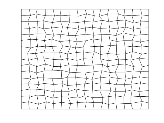
Figure 3: A nonuniform randomly perturbed quadrilateral triangulation

The tables containing numerical results are organized as follows: the parametric nonconforming elements in Tables 1 and  4, the nonparametric nonconforming elements with $\widetilde{c}=0$ in Tables 2 and  5, and those with $\widetilde{c}=1$ in Tables 3 and  6; the uniformly $\theta$-dependent trapezoidal meshes in Tables 1 –  3 and the nonuniform quadrilateral meshes in Tables 4 –  6.

We tested several different $\theta$’s, but the convergence behaviors were quite similar and thus we report only the case of $\theta=0.7$.

Numerical experiments were performed with increasing values of $\widetilde{c}$ such as 10, 100, 1000, and so on. The larger $\widetilde{c}$ values are chosen, the slower convergence is observed. We only present numerics for the two nonparametric elements with $\widetilde{c}=0$ and 1. At this point we recommend readers to use $\widetilde{c}=0$ for its simplicity.

As observed in the uniform mesh the convergence order is optimal for both elements and the values of numerical solutions are almost identical. In order to compare cost efficiency in a fair fashion, we computed nonparametric basis functions for each quadrilateral and applied the static condensation to circumvent bubble functions for parametric element also for each quadrilateral. From Table 7 we observe that when the mesh size $h$ is larger than 1/100, the nonparametric element is cheaper to use; however, the computing time ratios approach to 1 (still the use of nonparametric element seems to be cheaper), as the mesh size tends to decrease. These phenomena are perhaps due to the fact that the additional cost in static condensation for the parametric elements takes a less portion in the total computing time as the mesh size decreases.

h	DOF	$||u-u_{h}||_{0,\Omega}$	ratio	$||u-u_{h}||_{1,h}$	ratio
1/4	40	0.5284E-01	-	0.8532	-
1/8	176	0.1556E-01	1.76	0.4458	0.94
1/16	736	0.4184E-02	1.89	0.2274	0.97
1/32	3008	0.1096E-02	1.93	0.1147	0.99
1/64	12160	0.2810E-03	1.96	0.5756E-01	0.99
1/128	48896	0.7117E-04	1.98	0.2883E-01	1.00
1/256	196096	0.1791E-04	1.99	0.1443E-01	1.00

Table 1: Computational results for $\mathcal{NC}^{p}_{h,0}$ with $\theta=0.7$ for the elliptic problem.

h	DOF	$||u-u_{h}||_{0,\Omega}$	ratio	$||u-u_{h}||_{1,h}$	ratio
1/4	24	0.5437E-01	-	0.8221	-
1/8	112	0.1568E-01	1.79	0.4302	0.93
1/16	480	0.4145E-02	1.92	0.2213	0.96
1/32	1984	0.1084E-02	1.93	0.1124	0.98
1/64	8064	0.2788E-03	1.96	0.5659E-01	0.99
1/128	32512	0.7077E-04	1.98	0.2839E-01	1.00
1/256	130560	0.1783E-04	1.99	0.1422E-01	1.00

Table 2: Computational results for $\mathcal{NC}^{np}_{h,0}$ with $\theta=0.7$ and $\widetilde{c}=0$ for the elliptic problem

h	DOF	$||u-u_{h}||_{0,\Omega}$	ratio	$||u-u_{h}||_{1,h}$	ratio
1/4	24	0.5840E-01	-	0.8486	-
1/8	112	0.1655E-01	1.82	0.4452	0.93
1/16	480	0.4229E-02	1.97	0.2261	0.98
1/32	1984	0.1102E-02	1.94	0.1145	0.98
1/64	8064	0.2836E-03	1.96	0.5760E-01	0.99
1/128	32512	0.7212E-04	1.98	0.2887E-01	1.00
1/256	130560	0.1819E-04	1.99	0.1446E-01	1.00

Table 3: Computational results for $\mathcal{NC}^{np}_{h,0}$ with $\theta=0.7$ and $\widetilde{c}=1$ for the elliptic problem.

h	DOF	$||u-u_{h}||_{0,\Omega}$	ratio	$||u-u_{h}||_{1,h}$	ratio
1/4	40	0.3490E-01	-	0.7183	-
1/8	176	0.8663E-02	2.01	0.3657	0.97
1/16	736	0.2287E-02	1.92	0.1871	0.97
1/32	3008	0.5835E-03	1.97	0.9387E-01	0.99
1/64	12160	0.1481E-03	1.98	0.4721E-01	0.99
1/128	48896	0.3729E-04	1.99	0.2363E-01	1.00
1/256	196096	0.9350E-05	2.00	0.1183E-01	1.00

Table 4: Computational results for $\mathcal{NC}^{p}_{h,0}$ on the nonuniform randomly perturbed meshes for the elliptic problem.

h	DOF	$||u-u_{h}||_{0,\Omega}$	ratio	$||u-u_{h}||_{1,h}$	ratio
1/4	24	0.3594E-01	-	0.7363	-
1/8	112	0.8760E-02	2.04	0.3682	1.00
1/16	480	0.2290E-02	1.94	0.1873	0.98
1/32	1984	0.5834E-03	1.97	0.9386E-01	1.00
1/64	8064	0.1479E-03	1.98	0.4718E-01	0.99
1/128	32512	0.3725E-04	1.99	0.2362E-01	1.00
1/256	130560	0.9341E-05	2.00	0.1182E-01	1.00

Table 5: Computational results for $\mathcal{NC}^{np}_{h,0}$ on the nonuiform randomly perturbed meshes when $\widetilde{c}=0$ for the elliptic problem.

h	DOF	$||u-u_{h}||_{0,\Omega}$	ratio	$||u-u_{h}||_{1,h}$	ratio
1/4	24	0.3598E-01	-	0.7370	-
1/8	112	0.8752E-02	2.04	0.3684	1.00
1/16	480	0.2290E-02	1.93	0.1874	0.98
1/32	1984	0.5842E-03	1.97	0.9398E-01	1.00
1/64	8064	0.1481E-03	1.98	0.4725E-01	0.99
1/128	32512	0.3730E-04	1.99	0.2365E-01	1.00
1/256	130560	0.9353E-05	2.00	0.1184E-01	1.00

Table 6: Computational results for $\mathcal{NC}^{np}_{h,0}$ on the nonuniform randomly perturbed meshes when $\widetilde{c}=1$ for the elliptic problem.

h	$\theta=0.3$	$\theta=0.5$	$\theta=0.7$	Random mesh
1/8	0.6764	0.6764	0.6666	0.6571
1/16	0.6711	0.6621	0.6802	0.6712
1/32	0.6796	0.6761	0.6844	0.7022
1/64	0.7333	0.7285	0.7303	0.7344
1/128	0.7611	0.7656	0.7540	0.7275
1/256	0.8136	0.8296	0.7924	0.7875
1/512	0.9431	0.9170	0.8861	0.8415

Table 7: Ratio of computing time t($\mathcal{NC}^{np}_{h,0}$)/t$(\mathcal{NC}^{p}_{h,0})$ for the elliptic problem on uniform trapezoidal meshes with varying parameter $\theta$ and on nonuniform randomly perturbed meshes.

3.2 The incompressible Stokes equations

In this subsection, we apply $\mathcal{NC}^{np}_{h,0}$ to approximate each component of the velocity fields in solving the incompressible Stokes equations in two dimensions, while the piecewise constant element is employed to approximate the pressure.

Set $\Omega=(0,1)^{2}$ and consider the following Stokes equations:

$$\begin{split}-\Delta\mathbf{u}+\nabla p&=\mathbf{f}\qquad\mathrm{in}~{}\Omega,\\ \nabla\cdot\mathbf{u}&=0\qquad\mathrm{in}~{}\Omega,\\ \mathbf{u}&=0\qquad\mathrm{on}~{}\partial\Omega,\end{split}$$

where the force term $\mathbf{f}$ is generated by the following exact solution

$$\begin{split}\mathbf{u}(x_{1},x_{2})&=\left(\begin{array}[]{c}e^{x_{1}+2x_{2}}(x_{1}^{4}-2x_{1}^{3}+x_{1}^{2})(2x_{2}^{4}-4x_{2}^{2}+2x_{2})\\ -e^{x_{1}+2x_{2}}(x_{1}^{4}+2x_{1}^{3}-5x_{1}^{2}+2x_{1})(x_{2}^{4}-2x_{2}^{3}+x_{2}^{2})\end{array}\right),\\ p(x_{1},x_{2})&=-\sin 2\pi x_{1}\sin 2\pi x_{2}.\end{split}$$

Table 8 shows the numerical results on uniform trapezoidal meshes with $\theta=0.7$ and $\widetilde{c}=0.$ Similarly, Table 9 presents the results on the perturbed nonuniform meshes with $\widetilde{c}=0.$ From these numerical results, we observe the optimal convergence rates of $O(h^{2})$ and $O(h)$ for the velocity and pressure in $L^{2}$ norm, respectively. The numerical solutions in the case with $\widetilde{c}\neq 0$ behave similarly, whose tables are omitted to report.

h	DOF	$||\mathbf{u}-\mathbf{u}_{h}||_{0,\Omega}$	ratio	$||p-p_{h}||_{0,\Omega}$	ratio
1/4	63	0.1302E-01	-	0.2770	-
1/8	287	0.5424E-02	1.26	0.1898	0.55
1/16	1215	0.1631E-02	1.73	0.9571E-01	0.99
1/32	4991	0.4396E-03	1.89	0.4801E-01	1.00
1/64	20223	0.1130E-03	1.96	0.2410E-01	0.99
1/128	81407	0.2855E-04	1.98	0.1208E-01	1.00

Table 8: Computational results for $\mathcal{NC}^{np}_{h,0}$ with $\theta=0.7$ and $\widetilde{c}=0$ for the Stokes problem.

h	DOF	$||\mathbf{u}-\mathbf{u}_{h}||_{0,\Omega}$	ratio	$||p-p_{h}||_{0,\Omega}$	ratio
1/4	63	0.1205E-01	-	0.2960	-
1/8	287	0.3474E-02	1.79	0.1635	0.85
1/16	1215	0.9061E-03	1.94	0.8381E-01	0.96
1/32	4991	0.2332E-03	1.96	0.4216E-01	0.99
1/64	20223	0.5801E-04	2.00	0.2103E-01	1.00
1/128	81407	0.1455E-04	2.00	0.1052E-01	1.00

Table 9: Computational results for $\mathcal{NC}^{np}_{h,0}$ on the perturbed nonuniform mesh when $\widetilde{c}=0$ for the Stokes problem.

3.3 The planar linear elasticity problem

In this subsection, the nonparametric element $\mathcal{NC}^{np}_{h,0}$ is applied to approximate each component of the displacement fields for the planar linear elasticity problem with the clamped boundary condition.

Set $\Omega=(0,1)^{2}.$ For $(\mu,\lambda)\in[\mu_{0},\mu_{1}]\times[\lambda_{1},\infty),$ consider the following elasticity equations with homogeneous boundary condition:

$$\begin{split}-(\lambda+\mu)\nabla(\nabla\cdot\mathbf{u})-\mu\Delta\mathbf{u}&=\mathbf{f}\qquad\mathrm{in}~{}\Omega,\\ \mathbf{u}&=0\qquad\mathrm{on}~{}\partial\Omega,\end{split}$$

where the external force term $\mathbf{f}$ is generated by the following exact solution

$$\begin{split}u_{1}(x_{1},x_{2})&=\sin 2\pi x_{2}(-1+\cos 2\pi x_{1})+\frac{1}{1+\lambda}\sin\pi x_{1}\sin\pi x_{2},\\ u_{2}(x_{1},x_{2})&=-\sin 2\pi x_{1}(-1+\cos 2\pi x_{2})+\frac{1}{1+\lambda}\sin\pi x_{1}\sin\pi x_{2}.\end{split}$$

In order to check numerical locking phenomena, the Lamé parameters are chosen such that $(\mu,\lambda)=(1,1)$ and $(1,10^{5})$. The numerical results are presented in Tables 10 and  11 for both cases on uniform trapezoidal meshes with $\theta=0.7$ and $\widetilde{c}=0.$ Similar results are given in Tables 12 and  13 for both cases on the randomly perturbed meshes with $\widetilde{c}=0.$ One can easily observe from the numerical results that the nonparametric element $\mathcal{NC}^{np}_{h,0}$ can be used to solve planar elasticity problems with the clamped boundary condition optimally without numerical locking.

h	DOF	$||\mathbf{u}-\mathbf{u}_{h}||_{0,\Omega}$	ratio	$||\mathbf{u}-\mathbf{u}_{h}||_{1,h}$	ratio
1/4	48	0.3787	-	5.640	-
1/8	224	0.1074	1.81	2.941	0.93
1/16	960	0.2911E-01	1.88	1.524	0.94
1/32	3968	0.7521E-02	1.95	0.7712	0.98
1/64	16128	0.1906E-02	1.98	0.3870	0.99
1/128	65024	0.4793E-03	1.99	0.1937	1.00

Table 10: Computational results for $\mathcal{NC}^{np}_{h,0}$ with $\theta=0.7$, $\widetilde{c}=0$, $\mu=1$, and $\lambda=1$ for the elasticity problem.

h	DOF	$||\mathbf{u}-\mathbf{u}_{h}||_{0,\Omega}$	ratio	$||\mathbf{u}-\mathbf{u}_{h}||_{1,h}$	ratio
1/4	48	0.3781	-	5.631	-
1/8	224	0.1075	1.81	2.918	0.95
1/16	960	0.2900E-01	1.89	1.511	0.95
1/32	3968	0.7495E-02	1.95	0.7642	0.98
1/64	16128	0.1902E-02	1.98	0.3834	0.99
1/128	65024	0.4789E-03	1.99	0.1919	1.00

Table 11: Computational results for $\mathcal{NC}^{np}_{h,0}$ with $\theta=0.7$, $\widetilde{c}=0$, $\mu=1$, and $\lambda=10^{5}$ for the elasticity problem.

h	DOF	$||\mathbf{u}-\mathbf{u}_{h}||_{0,\Omega}$	ratio	$||\mathbf{u}-\mathbf{u}_{h}||_{1,h}$	ratio
1/4	48	0.2517	-	4.679	-
1/8	224	0.6530E-01	1.77	2.459	0.73
1/16	960	0.1724E-01	1.92	1.264	0.96
1/32	3968	0.4392E-02	1.97	0.6382	0.99
1/64	16128	0.1105E-02	1.99	0.3197	1.00
1/128	65024	0.2776E-03	1.99	0.1601	1.00

Table 12: Computational results for $\mathcal{NC}^{np}_{h,0}$ on the perturbed nonuniform mesh with $\widetilde{c}=0$, $\mu=1$, and $\lambda=1$ for the elasticity problem.

h	DOF	$||\mathbf{u}-\mathbf{u}_{h}||_{0,\Omega}$	ratio	$||\mathbf{u}-\mathbf{u}_{h}||_{1,h}$	ratio
1/4	48	0.2523	-	4.659	-
1/8	224	0.6591E-01	1.93	2.444	0.93
1/16	960	0.1746E-01	1.92	1.255	0.96
1/32	3968	0.4461E-02	1.97	0.6334	0.99
1/64	16128	0.1124E-02	1.99	0.3174	1.00
1/128	65024	0.2825E-03	1.99	0.1589	1.00

Table 13: Computational results for $\mathcal{NC}^{np}_{h,0}$ on the perturbed nonuniform mesh with $\widetilde{c}=0$, $\mu=1$, and $\lambda=10^{5}$ for the elasticity problem.

References

• [1] D. N. Arnold, D. Boffi, and R. S. Falk. Approximation by quadrilateral finite elements,. Math. Comp., 71:909–922, 2002.
• [2] S. C. Brenner and L. Y. Sung. Linear finite element methods for planar elasticity. Math. Comp., 59:321–338, 1992.
• [3] Z. Cai, J. Douglas, Jr., J. E. Santos, D. Sheen, and X. Ye. Nonconforming quadrilateral finite elements: A correction. Calcolo, 37(4):253–254, 2000.
• [4] Z. Cai, J. Douglas, Jr., and X. Ye. A stable nonconforming quadrilateral finite element method for the stationary Stokes and Navier-Stokes equations. Calcolo, 36:215–232, 1999.
• [5] Z. Chen. Projection finite element methods for semiconductor device equations. Computers Math. Applic., 25:81–88, 1993.
• [6] M. Crouzeix and P.-A. Raviart. Conforming and nonconforming finite element methods for solving the stationary Stokes equations. R.A.I.R.O.– Math. Model. Anal. Numer., R-3:33–75, 1973.
• [7] J. Douglas, Jr., J. E. Santos, D. Sheen, and X. Ye. Nonconforming Galerkin methods based on quadrilateral elements for second order elliptic problems. ESAIM–Math. Model. Numer. Anal., 33(4):747–770, 1999.
• [8] H. Han. Nonconforming elements in the mixed finite element method. J. Comp. Math., 2:223–233, 1984.
• [9] J. Hu and Z.-C. Shi. Constrained quadrilateral nonconforming rotated $Q_{1}$-element. J. Comp. Math., 23:561–586, 2005.
• [10] Y. Jeon, H. Nam, D. Sheen, and K. Shim. A nonparametric DSSY nonconforming quadrilateral element with maximal inf-sup constant. 2013. in preparation.
• [11] M. Köster, A. Ouazzi, F. Schieweck, S. Turek, and P. Zajac. New robust nonconforming finite elements of higher order. Applied Numerical Mathematics, 62(3):166–184, 2012.
• [12] R. Kouhia and R. Stenberg. A linear nonconforming finite element method for nearly incompressible elasticity and Stokes flow. Comput. Methods Appl. Mech. Engrg., 124(3):195–212, 1995.
• [13] C.-O. Lee, J. Lee, and D. Sheen. A locking-free nonconforming finite element method for planar elasticity. Adv. Comput. Math., 19(1–3):277–291, 2003.
• [14] P. Ming and Z.-C. Shi. Nonconforming rotated $Q_{1}$ element for Reissner-Mindlin plate. Math. Models Methods Appl. Sci., 11(8):1311–1342, 2001.
• [15] P. Ming and Z.-C. Shi. Two nonconforming quadrilateral elements for the Reissner–Mindlin plate. Math. Models Methods Appl. Sci., 15(10):1503–1517, 2005.
• [16] H. Nam, H. J. Choi, C. Park, and D. Sheen. A cheapest nonconforming rectangular finite element for the Stokes problem. Comput. Methods Appl. Mech. Engrg., 257:77–86, 2013.
• [17] C. Park and D. Sheen. $P_{1}$-nonconforming quadrilateral finite element methods for second-order elliptic problems. SIAM J. Numer. Anal., 41(2):624–640, 2003.
• [18] C. Park and D. Sheen. A quadrilateral Morley element for biharmonic equations. Numer. Math., 124(2): 395–413, 2013.
• [19] R. Rannacher and S. Turek. Simple nonconforming quadrilateral Stokes element. Numer. Methods Partial Differential Equations, 8:97–111, 1992.
• [20] Z.-C. Shi. An explicit analysis of Stummel’s patch test examples. Int. J. Numer. Meth. Engrg., 20(7):1233–1246, 1984.
• [21] Z. C. Shi. The FEM test for convergence of nonconforming finite elements. Math. Comp., 49(180):391–405, 1987.
• [22] S. Turek. Efficient solvers for incompressible flow problems, volume 6 of Lecture Notes in Computational Science and Engineering. Springer, Berlin, 1999.
• [23] M. Wang. On the necessity and sufficiency of the patch test for convergence of nonconforming finite elements. SIAM J. Numer. Anal., 39(2):363–384, 2001.
• [24] Z. Zhang. Analysis of some quadrilateral nonconforming elements for incompressible elasticity. SIAM J. Numer. Anal., 34(2):640–663, 1997.