Testing the Goodwin growth-cycle macroeconomic dynamics in Brazil

Abstract

This paper discusses the empirical validity of Goodwin’s (1967) macroeconomic model of growth with cycles by assuming that the individual income distribution of the Brazilian society is described by the Gompertz-Pareto distribution (GPD). This is formed by the combination of the Gompertz curve, representing the overwhelming majority of the population ($\sim\,$99%), with the Pareto power law, representing the tiny richest part ($\sim\,$1%). In line with Goodwin’s original model, we identify the Gompertzian part with the workers and the Paretian component with the class of capitalists. Since the GPD parameters are obtained for each year and the Goodwin macroeconomics is a time evolving model, we use previously determined, and further extended here, Brazilian GPD parameters, as well as unemployment data, to study the time evolution of these quantities in Brazil from 1981 to 2009 by means of the Goodwin dynamics. This is done in the original Goodwin model and an extension advanced by Desai et al. (2006). As far as Brazilian data is concerned, our results show partial qualitative and quantitative agreement with both models in the studied time period, although the original one provides better data fit. Nevertheless, both models fall short of a good empirical agreement as they predict single center cycles which were not found in the data. We discuss the specific points where the Goodwin dynamics must be improved in order to provide a more realistic representation of the dynamics of economic systems.

1 Introduction

It has been noted long ago by Karl Marx that capitalist production grows on cycles of booms and busts. During a boom, profits increase and unemployment decreases since the workers are able to get better jobs and higher salaries due to shortage of manpower to feed the growing production. However, this boom is followed by a bust since less unemployment reduces the profit margin, whose recovery is achieved by a higher unemployment and a reduction of the workers’ bargaining power. Smaller salaries increase the profit margin leading to renewed investment and then a new boom starts, being followed by another bust, and so on [1, Chap. 25, Sect. 1].

A century later Richard Goodwin [2] proposed a mathematical model which attempts to capture the essence of Marx’s dynamics described above. In this model the basic dynamics of a capitalist society, as qualitatively described by Marx, is modeled by means of a modified Lotka-Volterra model where predator and prey are represented by workers and capitalists. Goodwin replaced the classic Lotka-Volterra dynamics of number of predators and preys by two new variables $u$ and $v$, the former giving the workers’ share of total production, which is an indirect way of describing the profit margin of capitalists, and $v$ representing the employment rate, which is an indirect way of describing the share of those marginalized by the production, the unemployed workers, that is, the industrial reserve army of labor in Marx’s terminology. In a boom the employment rate $v$ increases and the workers’ share $u$ starts to increase after a time lag, meaning a decrease in profit margin. When employment rate is at its maximum this corresponds to the lowest profit margin, then the burst phase starts with a decrease in $v$. At this point $u$ had already started diminishing. The essence of the model is captured as a closed orbit in the $u$-$v$ phase space. Clearly these two variables are out of phase in time [3, pp. 458-464].

Although the brief description given above appears to indicate that Goodwin was able to capture Marx’s observations, the model has in fact several shortcomings, the most severe one being its inability to predict quantitatively the above described dynamics (see below). The model was presented simply as an heuristic reasoning capable of giving a mathematical dressing to Marx’s ideas. It was born out as a vision of the world rather than from a real-world data-inspired model in a physical sense. Despite this, or, perhaps, because of this, since its formulation Goodwin’s model has attracted considerable theoretical attention in some economic circles and several variations of the original model were proposed [see 4, 5, 6, 7, 8, 9, 10, 11, 12, 13, 14, 15, 16, 17, 18, and references therein].

However, interestingly enough, almost half a century after its proposal, attempts to actually test this model empirically are still extremely limited. Although Goodwin’s growth-cycle model is certainly influential in view of the number of theoretical follow-up papers cited above, studies seeking to establish its empirical soundness are limited only to Refs. [19, 20, 21, 22, 10, 23, 24, 25]. This is a surprisingly short list when we consider the time span since the model’s initial proposal. So little interest in empirically checking the model, especially among those who appear to have been seduced by its conceptual aspects, is even more surprising if we bear in mind that for the last 30 years or so we have been living in an era where large economic databases are easily available digitally, so large-scale checking of this model against empirical data ceased long ago to pose an insurmountable barrier. Besides, even the very few studies which actually attempted that, all point to severe empirical limitations of the model, ranging from partial qualitative acceptance to total quantitative rejection. From an econophysics viewpoint it is curious that a model with such a poor empirical record became so influential.

Despite this, the model does have some general empirical correspondence to reality on a qualitative level and this justifies further empirical studies with different databases, data handling methods and/or data type approaches. The basic aim must lie in identifying as clearly as possible where the model performs poorly in order to propose amendments and modifications. Any model, especially those theoretically seducing, can only remain of interest if it passes the test of experience, if it survives confronting its predictions with empirical data. If it does not survive this test the model must be modified, or abandoned.

This paper seeks to perform an empirical study of the Goodwin growth-cycle model using individual income data of Brazil. The study presented here was directly motivated by our previous experience in modeling Brazil’s income distribution, whose results suggested a Goodwin type oscillation in the share of the two income classes detected in the data [26, 27]. Building upon our previous experience with this database, we obtained yearly values of the two main variables of the Goodwin model, the labor share $u$ and the employment rate $v$. Nevertheless, differently from all previous approaches for testing Goodwin’s model, here the labor share was obtained by modeling the individual income distribution data with the Gompertz-Pareto distribution (GPD) and identifying $u$ with the Gompertzian, less wealthy, part of the distribution [27]. The employment rate was also estimated from the same database, that is, from Brazil’s income distribution, using the concept of effective unemployment.

We show that from 1981 to 2009 $u$ and $v$ do cycle in a form bearing similarities to what the Goodwin model predicts, that is, closed cycles. However, our results show the absence of a single cycling center and also are in complete disagreement with the ones for Brazil as reported by Ref. [25], whose analysis employed Harvie’s method [22]. In addition, we attempted to see if our findings bring empirical support to the Desai-Henry-Mosley-Pemberton (DHMP) extension of the original model [9]. Our results show that this particular variation of the Goodwin dynamics has some empirical soundness, although it provides a somewhat poorer data fit as compared to the original model and also leaves three parameters to be determined by other, still unknown, means than the ones studied here, whereas the original model leaves two parameters in a similar situation. We conclude that these two models provide partial qualitative and quantitative agreement with real data, at least as far as empirical data from Brazil are concerned, but both of them, and perhaps all variations of the original Goodwin growth-cycle dynamics, require important modifications and amendments before they can be considered viable representations of the real dynamics of economic systems.

The paper is organized as follows. Sect. 2 presents a brief review of the original Goodwin model and its DHMP extension, focusing mostly on their dynamical equations, although some discussion about the underlying economic hypotheses and foundations of the original model is also presented. In Sect. 3, after a short discussion about methodology, we review the main equations behind the GPD. Sect. 4 analyzes the individual income data of Brazil and presents the $u$-$v$ orbits in the 1981-2009 time period. Sect. 5 provides time variations of the employment rate as compared to workers’ share so that line fittings allow us to determine some of the unknown parameters of both models. Finally, Sect. 6 discusses the results and presents our conclusions.

2 The Goodwin growth-cycle macro-economic dynamics

2.1 The original growth-cycle model

The model proposed by Goodwin is essentially a Lotka-Volterra predator-prey system of first order ordinary differential equations which can be written as follows [2, 22, 9],

$$\dot{u}=\left[-\left(a+d\right)+hv\right]u,$$ (1)

$$\dot{v}=\left[\displaystyle\frac{100-u}{c}-\left(a+b\right)\right]v,$$ (2)

where the dot denotes the time differentiation $\mathrm{d}/\mathrm{d}t$. The five constants $a,b,c,d,h$ come from the economic hypotheses of the model and are supposed to obey the following conditions [3, 22],

$$\left\{\begin{array}[]{ll}c>0,\\ h>0,\\ (a+d)>0,\\ (a+b)\,c<100.\end{array}\right.$$ (3)

The solution of equations (1) and (2) produces a family of closed orbits with period $T$, all having the point $(u_{c},v_{c})$ as their unique center, according to the following equations [22],

$$\left\{\begin{array}[]{ll}u_{c}=100-(a+b)c,\\ v_{c}=(a+d)/h,\\ T={2\pi}\,\big{.}\big{/}{\sqrt{(a+d)[100/c-(a+b)]}}.\end{array}\right.$$ (4)

Since $u$ is the percentage share of labor, or workers, in national income and $v$ represents the proportion of labor force employed, they both should lie in the [0, 100] interval. Here we follow the normalization adopted in Refs. [26, 27] and shall refer to the maximum share, or proportion, as 100%. The upper singular point $v_{s}$ for the employment proportion is reached when $\dot{v}=0$, then $u_{s}=100-c(a+b)$. Similarly, when $\dot{u}=0$ we have $v_{s}=(a+d)/h$. However, if $(a+b)$ is negative, then $u_{s}>100$, which, in principle, should not be allowed (for a conceptually possible, but so far untested, exception, see Ref. [3], p. 461). Similarly, it is possible to have $v_{s}>100$.

In this model $u$ represents the population density of predators whereas $v$ represents the prey population density. This can be seen as follows. When $u=0$, $\dot{u}=0$ and $\dot{v}>0$. In other words, $u$ remains equal to zero whereas $v$ grows without bound, a situation happening to the prey population $v$ in the absence of predators $u$. On the other hand, when $v=0$, equations (1) and (2) together with conditions (3) show that $\dot{v}=0$ and $\dot{u}<0$. So, without prey ($v=0$), the predator population decreases ($\dot{u}<0$).

The model is defined in terms of five parameters. However, once they are grouped as below,

$$\left\{\begin{array}[]{ll}a_{1}=(a+d),\\ a_{2}=(100/c)-(a+b),\\ b_{1}=h,\\ b_{2}=100/c,\end{array}\right.$$ (5)

they allow equations (1) and (2) to be rewritten in the form of the classical Lotka-Volterra equations [3],

$${\dot{u}}/{u}=-a_{1}+b_{1}\,v,$$ (6)

$${\dot{v}}/{v}=a_{2}-b_{2}\,u,$$ (7)

that is, in terms of four parameters which could, in principle, be determined observationally, provided that both variables and their derivatives are obtained from real data.

2.2 The Desai-Henry-Mosley-Pemberton (DHMP) extension

Desai et al. [9] noted that the original Goodwin model can produce solutions outside the $u$-$v$ domain $[0,100]\times[0,100]$ because, as seen above, both $u_{s}$ and $v_{s}$ can grow above 100. This is the main reason which led them to propose a modified version of Goodwin’s original model, dubbed here as the DHMP extension. They also relaxed two other economic hypotheses assumed in the original model. So, in the DHMP extension all profits are not always invested and the Phillips curve, relating unemployment and inflation rate, is non-linear. Thus, the final equations yield,

$$\dot{u}=\left[-(\bar{a}+\bar{d})+\bar{h}{(100-v)}^{\delta}\right]u,$$ (8)

$$\dot{v}=\left\{\left[-\lambda\ln(100-\bar{u})-(\bar{a}+\bar{b})\right]+\lambda\ln(\bar{u}-u)\right\}v,$$ (9)

where $\bar{a}$, $\bar{b}$, $\bar{d}$, $\bar{h}$, $\delta$, $\lambda$, $\bar{u}$ are constants obeying the following constraints,

$$\left\{\begin{array}[]{ll}\delta>0,\\ \lambda>0,\\ u<\bar{u}<100,\\ \bar{h}<(\bar{a}+\bar{d}),\\ (\bar{a}+\bar{b})<\lambda\ln\left(\displaystyle\frac{\bar{u}}{100-\bar{u}}\right),\\ \displaystyle\left(\frac{\bar{u}}{100-\bar{u}}\right)>1.\end{array}\right.$$ (10)

Ref. [9] gives a clear meaning to the parameter $\bar{u}$ as being “the maximum share of labor that capitalists would tolerate”, “typically” given by the last constraint equation in the set of expressions (10) above. Clearly this implies that $\bar{u}>50$%. One must also note that both the original Goodwin model and its DHMP extension consider that the labor share and profits are not given in terms of money, but in real terms. As we shall see below, this requirement does not pose a problem for our approach since our variables are currency independent [see 26].

As seen above, the DHMP extension of Goodwin’s growth cycle model is defined by seven parameters which can be grouped as below,

$$\left\{\begin{array}[]{ll}\bar{a}_{1}=(\bar{a}+\bar{d}),\\ \bar{a}_{2}=\lambda\ln(100-\bar{u})+(\bar{a}+\bar{b}),\\ \bar{b}_{1}=\bar{h},\\ \bar{b}_{2}=\lambda,\end{array}\right.$$ (11)

allowing us to rewrite equations (8) and (9) as follows,

$${\dot{u}}/{u}=-\bar{a}_{1}+\bar{b}_{1}\,V^{\delta},$$ (12)

$${\dot{v}}/{v}=-\bar{a}_{2}+\bar{b}_{2}\,\ln\mathcal{U},$$ (13)

where

$$\mathcal{U}\equiv\bar{u}-u,$$ (14)

and the unemployment rate given by,

$$V\equiv 100-v.$$ (15)

Although the basic motivation for the DHMP extension was to avoid the variables of the model having values above 100%, this difficulty can be avoided if both $u$ and $v$ are defined by real data, in which case the desired threshold will be achieved by construction. Besides, the DHMP model has the additional disadvantage of requiring seven, rather than five, unknown parameters.

2.3 Interpretation of the conflicting variables

As seen above the Goodwin model is essentially a predator - prey type one and this means that its two variables represent the opposing, but interdependent, nature of a predator - prey conflict. This is the reason why this model is also known as “Goodwin’s class struggle model.” The nature of this “struggle” arises from the possible ways we interpret its variables.

On one hand, the employment rate $v$ can be identified with the workers’ class and the profit share of the “capitalists” is then given by,

$$U\equiv 100-u.$$ (16)

In other words, $U$ is the share of total national income obtained by the class that controls the capital, the investors. In this case the conflict is between the workers and the investors (capitalists). That can be seen in the light of a change of variables such that when $u=0$, $\dot{u}=0$, $\dot{{U}}=0$ and $\dot{v}>0$, meaning that when the profit ${U}$ attained by investors remains constant, i.e., $\dot{U}=0$, the workers’ share $v$ grows without bound and represents the prey, whereas the investors ${U}$ are in the role of predators. Here ${U}$ is assumed to have a maximum value equal to 100%.

On the other hand, following Solow [21], employed workers can be identified with the workers’ share $u$ and unemployed workers with the variable $V$. In this case the conflict is between employed and unemployed workers. When $u=0$, $\dot{u}=0$ and $\dot{V}<0$. This is consistent with the employed workforce $u$ in the role of prey, the unemployed workers $V$ being identified with the predators and the investors as passive non-players.

However, these interpretations should not be taken at their face values as they are dependent on the conditions given by equations (3). Such parameter constraints were, however, not established from an analysis of real-world data, but came from entirely heuristic, and so far very poorly tested, reasoning. In addition, since as seen above the variables $u$ and $v$ can be identified in more than one way, this means that such interpretations must be done with care and always in the light of real-world data analysis and not on a speculative basis. As further emphasis of these difficulties, one may even argue that the constants of the model may not be constants at all, but time dependent variables themselves (see below).

2.4 Origins of the Goodwin model

As noted above, when developing his model Goodwin aimed at putting in mathematical form Marx’s conceptual ideas about cycles in capitalism. However, as pointed out by Keen [28], Goodwin also wished to show how cyclical behavior could arise from very simple economic hypotheses. Next we shall present a simple derivation of the model in order to highlight that it results from an extremely simplified representation of the economy.

Let $K$ be the amount of fixed capital (plant and equipment) and $Y$ the output that an economy can generate. The output to capital ratio $\sigma$ clearly varies over time in a country, but let us consider it a constant as a first approximation and write it as follows,

$$\sigma={K}/{Y}.$$ (17)

If $L$ is the amount of labor for a given output, one can also assume as first approximation a constant output to labor ratio $a$, that is,

$$a={Y}/{L}.$$ (18)

The amount of labor can be written in terms of the population $N$ and the employment rate $v$ as follows,

$$L=Nv.$$ (19)

Let $w$ be the average wage value. Then the wage bill, that is, the total amount of wages in an economy is given by,

$$W=wL.$$ (20)

At a first approximation the employment rate can be related to the rise of wages as follows,

$${\dot{w}}/{w}=f_{1}(v).$$ (21)

Since the wage share $u$ is given by,

$$u={wL}/{Y},$$ (22)

remembering that $a$ is constant, equation (21) becomes,

$${\dot{u}}/{u}=f_{1}(v).$$ (23)

This expression reduces to equation (6) if $f_{1}(v)$ is assumed to be a linear function.

The profit level $P$ is given by,

$$P=Y-W.$$ (24)

As a first approximation all profits are invested, so the profit share $P/Y$ is the investment $\Upsilon$. Hence,

$$\Upsilon={P}/{Y}=100-({W}/{Y})=100-u=U.$$ (25)

Here the unit was changed to 100% due to our previous choice of normalization. The profit rate $\pi$ is given by,

$$\pi={P}/{K},\;\;\;\Longrightarrow\;\;\;\Upsilon=\sigma\pi=100-u,$$ (26)

which can be rewritten in functional form as below,

$$\Upsilon=f_{2}(u).$$ (27)

Investment is also the rate of change of capital $\dot{K}/K$. So,

$$\Upsilon=\frac{\dot{K}}{K}=\frac{\dot{Y}}{Y}=\frac{\dot{v}}{v}+\mathrm{const.}\,,$$ (28)

where the constant comes from the hypothesis of a steady labor supply, e.g., $L$ changes exponentially. Summing up we have that,

$${\dot{v}}/{v}=f_{2}(u),$$ (29)

which reduces to equation (7) if $f_{2}(u)$ is assumed linear.

Clearly the model results from extremely simple specifications of the economy. But, it is so simple that it cannot reproduce the frequency properties of output growth in a certain time period or the distribution of recession sizes and duration. However, the dynamic stochastic general equilibrium (DSGE) models of cycles adopted by current neoclassical economics cannot do so either [29, 30, 31], hence what is remarkable is that the very restricted model proposed by Goodwin finds any empirical support in real data [28].

3 The Gompertz-Pareto income distribution

Econophysics is a new research field whose problems interest both economists and physicists. However, when physicists approach a problem traditionally dealt with by economists, they do so under a very different modeling perspective. Although it is uncommon to find methodological issues discussed in physics papers, considering the hybrid nature of econophysics and the theoretical crisis of the current mainstream economic thought [29, 30, 31, 32, 33, 34, 35, 36, 37, 38, 39, 40, 41, 42], it is worthwhile to emphasize the differences in methodological perspectives between physics and economics regarding model building and, especially, model abandoning. We have already expressed some of our thoughts on this topic in Ref. [26, Sect. 3], but a few more words are worth saying before we review our approach to the income distribution problem.

Econophysics was born and remains a branch of physics [43, 44, 45], employing, therefore, its centuries old proven epistemological methodology. It considers a scientific theory as being made by laws of nature, which are theoretical constructs, often expressed in mathematical language, that capture regularities, processes, structures and interrelationships of reality. Successful physical laws provide good empirical representations, or images, of the real world, of nature, and allow us to reach predictions regarding the outcomes of processes that do go on in nature. However, by being images of nature, these laws are obviously limited and, hence, they will always provide imperfect representations. The only way we can ascertain how imperfect they are is by practice, i.e., by creating pragmatic measures of the adequacies of these laws, always empirically comparing their predictions with what occurs in the real world [46]. In other words, good laws provide good predictions, bad laws provide bad predictions. This has nothing to do with the extensive use of mathematics by physical theories. Mathematics is a language, a tool of formal logic, and by itself has no a priori relationship with physical, or social, reality. Physicists choose if and which mathematical tools are required to express something observed in nature.

Since our understanding of the theories behind these laws changes with time, the same occurring with the measures of adequacies due to technological advances, we must keep measuring the adequacies of these laws by perfecting old measures as well as creating new ones, that is, constantly updating our theories and models through practice in order to find their limits of validity. The theoretical aspects behind these laws, even their metaphysical presuppositions, must also be perfected by shedding the inappropriate elements so that the appropriate residue remains, in a process very similar to Darwin’s natural selection. And, if there is no appropriate residue left the theoretical construct is abandoned, becoming extinct [49]. Under this viewpoint, a model is a more restricted theoretical construct, taking one or two elements above – regularities, processes, structures and interrelationships –, but not all of them. Nevertheless, a model is also subject to measures of adequacy and since they incorporate less elements than a theory, it suffers a more rapid process of perfection by selection as well as extinction.

Physicists have been following this methodological approach for centuries and as a consequence they have amassed a large number of physical theories that were perfected by generations of physicists, who kept their appropriate kernels but changed their original elements in various degrees, and also to many other theories which are now superseded. Theoretical pluralism is tacitly accepted as an essential element for the development of physics. Real science starts from observation of nature, either physical or social, and any theoretical discussion must keep referring back to empirics, a factor that limits and guides any theoretical debate, leading to healthy refining, replacing or even abandoning of theories and models [50].

However, it seems that this methodological viewpoint regarding model checking has not been adopted by a sizable number of economists. Econophysicists are often perplexed to witness how often economists confuse their models with reality, showing a behavior which was already described as ‘scientific dogmatism’ [46]. Thus, they would often disregard startling obvious empirical facts rather than change or dismiss their inappropriate theories or models [51, 52], showing to a large extent an absolute devotion to theoretical economic constructs, especially an empirically unwarranted obsession with equilibrium, in parallel to little or no empirical interest, often keeping such a theoretical worship even when empirical evidence that might support the theory is absent. Worse still, even when there is evidence that directly contradicts what would be predicted to occur by applying the theories [53, pp. 2-5]. Some would say this phenomenon is due to ‘ideological assumptions’, disguised visions of the world under scientific pretenses [48]. Others call this behavioral mode ‘cargo cult economics’ [54] in reference to the famous Feynman speech about methodologically inadequate, or false science [55, 56]. Nevertheless, the epistemological ideas above, adopted by physicists a long time ago, are apparently being slowly absorbed into the economic thought [57, 58].

Having stated our methodological viewpoints, next we shall review the basic hypotheses and equations behind the GPD as advanced in Refs. [26, 27].

3.1 Definitions

Let $\mathcal{F}(x)$ be the cumulative income distribution giving the probability that an individual receives an income less than or equal to $x$. Then the complementary cumulative income distribution $F(x)$ gives the probability that an individual receives an income equal to or greater than $x$. It then follows that $\mathcal{F}(x)$ and $F(x)$ are related as follows,

$$\mathcal{F}(x)+F(x)=100,$$ (30)

where the maximum probability is taken to be 100%. Here $x$ is a normalized income obtained by dividing the nominal income values by some suitable nominal income average [26]. If both functions $\mathcal{F}(x)$ and $F(x)$ are continuous and have continuous derivatives for all values of $x$, we have that,

$${\mathrm{d}}\mathcal{F}(x)/{\mathrm{d}}x=f(x),\;\;\;\;{\mathrm{d}}F(x)/{\mathrm{d}}x=-f(x),$$ (31)

and

$$\int_{0}^{\infty}f(x):{\mathrm{d}}x=100,$$ (32)

where $f(x)$ is the probability density function of individual income. Thus, $f(x),{\mathrm{d}}x$ is the fraction of individuals with income between $x$ and $x+{\mathrm{d}}x$. The equations above lead to the following results,

$$\mathcal{F}(x)-\mathcal{F}(0)=\int_{0}^{x}f(w)\>{\mathrm{d}}w,\qquad F(x)-F(\infty)=\int_{x}^{\infty}f(w)\>{\mathrm{d}}w,$$ (33)

whose boundary conditions are,

$$\left\{\begin{array}[]{lclcl}\mathcal{F}(0)&=&{F}(\infty)&\cong&0,\\ \mathcal{F}(\infty)&=&{F}(0)&\cong&100.\end{array}\right.$$ (34)

Clearly both $\mathcal{F}(x)$ and $F(x)$ vary from 0 to 100.

3.2 The Gompertz-Pareto distribution (GPD)

The GPD was proposed in Ref. [26] and discussed in detail in Ref. [27]. Its complementary cumulative distribution is formed by the combination of two functions which can be identified with the two main classes forming most modern societies, workers and investors (capitalists). The first component describes the lower part of the distribution, that is, those who survive solely on their wages, the workers, and is given by a Gompertz curve. The second component of the complementary cumulative distribution describes the tail of the distribution by means of the Pareto power law and represents the investors, that is, the rich capitalists. Then we have that,

$$F(x)=\left\{\begin{array}[]{lcllc}G(x)&=&{\mathrm{e}}^{\displaystyle{\mathrm{e}}^{(A-Bx)}},&\;\;(\>0\leq x<x_{\scriptstyle t}),&\;\mbox{(Gompertz)}\\ \\ P(x)&=&{(x_{\scriptstyle t})}^{\alpha}\;{\mathrm{e}}^{\displaystyle{\mathrm{e}}^{(A-Bx_{\scriptstyle t})}}\;x^{-\alpha},&\;\;(x_{\scriptstyle t}\leq x\leq\infty),&\;\mbox{(Pareto)}\\ \end{array}\right.$$ (35)

and the cumulative income distribution may be written as below,

$$\mathcal{F}(x)=\left\{\begin{array}[]{ll}\mathcal{G}(x)=100-{\mathrm{e}}^{\displaystyle{\mathrm{e}}^{(A-Bx)}},&\;\;(\>0\leq x<x_{\scriptstyle t}),\\ \\ \mathcal{P}(x)=100-{(x_{\scriptstyle t})}^{\alpha}\;{\mathrm{e}}^{\displaystyle{\mathrm{e}}^{(A-Bx_{\scriptstyle t})}}\;x^{-\alpha},&\;\;(x_{\scriptstyle t}\leq x\leq\infty).\\ \end{array}\right.$$ (36)

Here $x_{\scriptstyle t}$ is the income value threshold of the Pareto region, $\alpha$ is the Pareto index describing the slope of the power law tail, $B$ is a third parameter characterizing the slope of the Gompertz curve and $A$ is a number whose value is set by boundary conditions, as follows. Since $G(x)=\exp\left[\exp(A-Bx)\right]$, the condition (34) implies $G(0)=100$, then we have that,

$$A=\ln\left(\ln 100\right)=1.5272\,.$$ (37)

The term ${(x_{\scriptstyle t})}^{\alpha}\;{\mathrm{e}}^{\displaystyle{\mathrm{e}}^{(A-Bx_{\scriptstyle t})}}$ is the normalization constant of the Pareto power law and comes as a consequence of condition (32), as well as the continuity of functions (35) across the frontier between the Gompertz and Pareto regions, defined to be $x=x_{t}$.

The equations above allow us to find the expressions for the probability density income distribution,

$$f(x)=\left\{\begin{array}[]{lclc}g(x)&=&B\;{\mathrm{e}}^{(A-Bx)}\;{\mathrm{e}}^{\displaystyle{\mathrm{e}}^{(A-Bx)}},&\;\;(\>0\leq x<x_{\scriptstyle t}),\\ \\ p(x)&=&\alpha\;{(x_{\scriptstyle t})}^{\alpha}\;{\mathrm{e}}^{\displaystyle{\mathrm{e}}^{(A-Bx_{\scriptstyle t})}}\;x^{{}^{\scriptstyle-(1+\alpha)}},&\;\;(x_{\scriptstyle t}\leq x\leq\infty),\\ \end{array}\right.$$ (38)

as well as the average income of the whole population described by the GPD,

$$\langle x\rangle=\frac{1}{100}\int_{0}^{\infty}x\>f(x)\>{\mathrm{d}}x=\frac{1}{100}\left[\mathcal{I}(x_{t})+\frac{\alpha\>x_{\scriptstyle t}}{(\alpha-1)}{\mathrm{e}}^{\displaystyle{\mathrm{e}}^{(A-Bx_{t})}}\right],$$ (39)

where,

$$\mathcal{I}(x)\equiv\int_{0}^{x}w\,g(w)\,{\mathrm{d}}w=\int_{0}^{x}w\>B\>{\mathrm{e}}^{(A-Bw)}\;{\mathrm{e}}^{\displaystyle{\mathrm{e}}^{(A-Bw)}}{\mathrm{d}}w.$$ (40)

The parameters $\alpha$, $x_{\scriptstyle t}$ and $B$ are all positive and they fully characterize the GPD. However, due to convergence requirements [26], the expression (39) for the average income is only valid if $\alpha>1$. Both $\alpha$ and $B$ can be determined by linear data fitting since equations (35) can be linearized. However, $x_{\scriptstyle t}$ is independently found under the constraint that the boundary condition (37) is satisfied to whatever degree of precision the available data allow.

The Lorenz curve of the GPD has its X-axis given by the cumulative income distribution function $\mathcal{F}(x)$, whereas the first-moment distribution function $\mathcal{F}_{1}(x)$ defines its Y-axis. Accordingly, they can be written as follows [27],

$$\mathcal{F}(x)=\int_{0}^{x}f(w)\>{\mathrm{d}}w=\left\{\begin{array}[]{lr}100-{\mathrm{e}}^{\displaystyle{\mathrm{e}}^{(A-Bx)}},&(0\leq x<x_{t}),\\ \\ 100-{(x_{t})}^{\alpha}\>{\mathrm{e}}^{\displaystyle{\mathrm{e}}^{(A-Bx_{t})}}x^{\,-\alpha},&\;\;\;(x_{t}\leq x<\infty),\end{array}\right.$$ (41)

and

$$\mathcal{F}_{1}(x)=\frac{1}{\langle x\rangle}\int_{0}^{x}w\>f(w)\>{\mathrm{d}}w=\left\{\begin{array}[]{lr}\displaystyle\frac{\mathcal{I}(x)}{\langle x\rangle}\,,&(0<x<x_{t}),\vspace{4mm}\\ 100+\displaystyle\frac{\displaystyle\alpha\,{(x_{t})}^{\alpha}}{\displaystyle(1-\alpha)}\>\frac{{\mathrm{e}}^{\displaystyle{\mathrm{e}}^{(A-Bx_{t})}}}{\langle x\rangle}\;{x^{(1-\alpha)}},&\;\;\;(x_{t}\leq x<\infty;).\end{array}\right.$$ (42)

Thus, $\mathcal{F}_{1}(x)$ varies from 0 to 100 as well. The Lorenz curve is usually represented in a unit square, but the normalization (32) implies that the square where the Lorenz curve is located has area equal to $10^{4}$.

The Gini coefficient under the currently adopted normalization is written as,

$$Gini=1-2\times 10^{-4}\int_{0}^{\infty}\mathcal{F}_{1}(x)\>f(x)\>{\mathrm{d}}x.$$ (43)

Considering now equations (38) and (42), the Gini coefficient has the following expression in the GPD,

$$Gini=1-2\times 10^{-4}\left\{\frac{B}{\langle x\rangle}\int\limits_{0}^{x_{t}}\mathcal{I}(x)\>{\mathrm{e}}^{(A-Bx)}{\mathrm{e}}^{\displaystyle{\mathrm{e}}^{(A-Bx)}}{\mathrm{d}}x+100\>{\mathrm{e}}^{\displaystyle{\mathrm{e}}^{(A-Bx_{t})}}+\frac{\alpha^{2}\>{x_{t}}\>{\mathrm{e}}^{2\,\displaystyle{\mathrm{e}}^{(A-Bx_{t})}}}{\langle x\rangle(\alpha-1)(1-2\alpha)}\right\}.$$ (44)

As discussed in [27], we can define the percentage share of the Gompertzian part of an income distribution described by the GPD by means of equation (42). This quantity may then be written as follows,

$$u=\mathcal{F}_{1}(x_{t})=100-\frac{\alpha}{(\alpha-1)}\frac{x_{t}}{\langle x\rangle}{\mathrm{e}}^{\displaystyle{\mathrm{e}}^{(A-Bx_{t})}}.$$ (45)

Hence, we identity the percentage share of the lower income strata described by the GPD with Goodwin’s labor share $u$. Note that by doing so, $u$ no longer represents the industrial reserve army of labor, but in fact the relative surplus population since the latter includes not only the unemployed, but also those unable to work. Such identification allows the description of the Goodwin variables in terms of measurable quantities connected to different income classes whose empirical values can be obtained, for instance, from the Lorenz curves. This connection can be made clearer by the inversion of equation (45),

$$\frac{1}{\alpha}=1-\left[\frac{\displaystyle u\,x_{t}\,{\mathrm{e}}^{\displaystyle{\mathrm{e}}^{(A-Bx_{t})}}}{\displaystyle(100-u)\mathcal{I}\,(x_{t})}\right].$$ (46)

Due to the high non-linearity of this expression one can only use it to determine $\alpha$ if the values of $u$, $B$ and $x_{t}$ are known to a very high degree of accuracy.

The equation (46) links the Pareto index $\alpha$ to parameters which are solely determined in the Gompertzian segment of the distribution: the cutoff value $x_{t}$, the Gompertzian percentage share $u$ and its distribution slope $B$. In other words, equation (46) links the income distribution of the lower and upper classes forming a society, showing clearly their dynamical inter-dependency. If we consider that temporal changes in the income distribution do take place, we can no longer consider these quantities as parameters. Some of them, or perhaps all of them, ought to be time dependent variables (see below).

The GPD requires $\alpha>0$. In addition, an average income is only possible if $\alpha>1$. Considering these two conditions in equation (46) we conclude that,

$$0<\left[\frac{\displaystyle u\,x_{t}\,{\mathrm{e}}^{\displaystyle{\mathrm{e}}^{(A-Bx_{t})}}}{\displaystyle(100-u)\mathcal{I}\,(x_{t})}\right]<1\;\;\;\;\;\mbox{and}\;\;\;\;\;u<100.$$ (47)

Remembering equation (16) the last condition is equivalent to $U>0$, which means that an income distribution described by the GPD is only possible in a system where investors have a nonzero share of the total income.

3.3 Exponential approximation

As shown in Refs. [26, 27], the upper part of the Gompertz curve can be approximated by an exponential and this allows us to take this subdivision of the Gompertz curve as representing the middle class present in most societies. In other words, in this approach of the income distribution characterization of a society we assume that the middle class is just the upper echelon of the wage labor class. Thus, for $Bx>A$, ${\mathrm{e}}^{-Bx}<1$ and $x<x_{t}$ we have that,

$$\left\{\begin{array}[]{ll}G(x)\approx 99+{\mathrm{e}}^{-Bx},\\ \mathcal{G}(x)\approx 1-{\mathrm{e}}^{-Bx},\\ g(x)\,\approx B\;{\mathrm{e}}^{-Bx},\end{array}\right.$$ (48)

which are already normalized to obey the boundary conditions (34). If the lower stratum of a society is formed essentially by a very large middle class, one can in principle write all equations shown in Sect. 3.2 in terms of the approximations (48), although in such a case we can expect a certain degree of distortion in the distribution since all modern societies seem to have a certain percentage of very poor people, however small this percentage may be.

4 Cycles in the income and employment data of Brazil

Publicly available individual income distribution data of the Brazilian population have allowed Moura Jr. and Ribeiro [26] to determine the GPD parameters from 1978 to 2005 after a careful handling of the data. Chami Figueira, Moura Jr. and Ribeiro [27] extended this analysis to include income data for 2006 and 2007, as well as showing how the GPD produces results compatible with those obtained directly from the raw data, that is, without assuming the GPD, with error margins up to 7%. In this work we further extend these two previous analyzes to include data for 2008 and 2009, but disregarding the results for 1978 and 1979 due to their unreliability [27].

Table 1 presents the three GPD parameters $B$, $x_{t}$ and $\alpha$ followed by the unemployment rate $[V]$, Gini coefficient and the percentage share of the Gompertzian component of the distribution. $B$ and $\alpha$ were obtained by linear data fitting whereas $x_{t}$ was determined such that a linear fit would produce the boundary condition (37) with discrepancy of about 2%. Lorenz curves were generated from the raw distribution for each year allowing the calculation of the Gini coefficient without assuming the GPD, denoted here as $[Gini]$ in order to distinguish it from the one obtained assuming the GPD in equation (44). Once $x_{t}$ was found it became possible determine $[u]$ directly from the raw data, that is, without using equation (45). Similarly, $[V]$ denotes the unemployment data without any distribution assumptions, $[v]$ is obtained using equation (15) and $x_{d}$ is the unemployment income threshold used to calculate $[V]$ (see below). The time derivatives are given by the expressions,

$$\dot{[u]}=\frac{{\mathrm{d}}}{{\mathrm{d}}t}[u]\,,\;\;\;\;\;\dot{[v]}=\frac{{\mathrm{d}}}{{\mathrm{d}}t}\left(100-[V]\right).$$ (49)

Table 1: Data for Brazil from 1981 to 2009. Values in brackets mean that they were evaluated without using the GPD parameters, that is, directly from the raw data. This table contains the GPD parameters $B$, $x_{t}$ and $\alpha$ for the individual income, unemployment income threshold $x_{d}$, unemployment rate $[V]$, Gini coefficient, percentage share $[u]$ of the Gompertzian component (workers’ share), employment rate $[v]$ and time derivatives of the last two quantities, as given by equations (49). The results from 1981 to 2007 had already appeared in [26, 27] whereas those for 2008 and 2009, as well as the ones for employment and unemployment, are new. The time derivatives $\dot{[u]}$ and $\dot{[v]}$ were calculated numerically using equation (51). Since there were no income samplings in 1991, 1994 and 2000 [see 26], some results for these years were obtained by numerical interpolation.

year	$B$	$x_{\scriptstyle t}$	$\alpha$	$x_{d}$	$[V]\,(\%)$	$[Gini]$	$[u]\,(\%)$	$\dot{[u]}\,(\%/\mbox{year})$	$[v]\,(\%)$	$\dot{[v]}\,(\%/\mbox{year})$
1981	$0.342\pm 0.016$	7.533	$2.839\pm 0.091$	$0.182$	$14.8$	$0.574$	$87.7$		$85.2$
1982	$0.342\pm 0.015$	7.473	$2.677\pm 0.042$	$0.174$	$14.5$	$0.581$	$87.2$	$+1.08$	$85.5$	$-0.20$
1983	$0.330\pm 0.010$	6.910	$2.636\pm 0.081$	$0.175$	$14.5$	$0.584$	$85.5$	$-0.04$	$85.5$	$-1.06$
1984	$0.332\pm 0.013$	7.388	$2.839\pm 0.072$	$0.170$	$12.4$	$0.576$	$87.2$	$-0.17$	$87.6$	$-1.32$
1985	$0.329\pm 0.010$	7.490	$2.656\pm 0.093$	$0.154$	$11.8$	$0.589$	$85.8$	$+0.99$	$88.2$	$-2.22$
1986	$0.344\pm 0.013$	7.112	$2.567\pm 0.065$	$0.127$	$7.9$	$0.580$	$85.2$	$-0.05$	$92.1$	$-1.16$
1987	$0.343\pm 0.016$	7.626	$2.724\pm 0.057$	$0.127$	$9.5$	$0.592$	$85.9$	$-0.08$	$90.5$	$+2.11$
1988	$0.324\pm 0.014$	8.140	$2.874\pm 0.125$	$0.133$	$12.1$	$0.609$	$85.4$	$+1,74$	$87.9$	$+0,17$
1989	$0.317\pm 0.010$	7.856	$2.428\pm 0.079$	$0.111$	$9.9$	$0.628$	$82.5$	$-0.23$	$90.1$	$-2.35$
1990	$0.335\pm 0.015$	8.074	$2.636\pm 0.053$	$0.099$	$7.4$	$0.605$	$85.9$	$-1.98$	$92.6$	$+0.48$
1991					$10.8$		$86.4$	$-0.57$	$89.2$	$+3.37$
1992	$0.364\pm 0.020$	7.635	$2.636\pm 0.063$	$0.162$	$14.2$	$0.578$	$87.0$	$+1.18$	$85.8$	$+0.53$
1993	$0.330\pm 0.008$	7.674	$2.567\pm 0.042$	$0.137$	$11.9$	$0.599$	$84.1$	$+1.01$	$88.1$	$-2.54$
1994					$9.1$		$85.0$	$-0.92$	$90.9$	$-2.75$
1995	$0.333\pm 0.012$	7.887	$2.777\pm 0.106$	$0.098$	$6.4$	$0.596$	$85.9$	$-0.86$	$93.6$	$-0.63$
1996	$0.347\pm 0.020$	8.163	$2.749\pm 0.107$	$0.096$	$7.8$	$0.598$	$86.7$	$-0.12$	$92.2$	$+0.43$
1997	$0.338\pm 0.015$	7.935	$2.617\pm 0.052$	$0.099$	$7.2$	$0.598$	$86.1$	$+1.09$	$92.8$	$-0.29$
1998	$0.326\pm 0.009$	7.628	$2.677\pm 0.031$	$0.103$	$7.3$	$0.597$	$84.5$	$+0.08$	$92.7$	$+0.25$
1999	$0.331\pm 0.013$	7.811	$2.777\pm 0.068$	$0.107$	$7.7$	$0.590$	$86.0$	$-0.53$	$92.3$	$+0.55$
2000					$8.4$		$85.6$	$+0.40$	$91.6$	$+0.66$
2001	$0.335\pm 0.011$	7.774	$2.724\pm 0.205$	$0.122$	$9.0$	$0.592$	$85.2$	$-0.41$	$91.0$	$-0.24$
2002	$0.339\pm 0.015$	7.878	$2.500\pm 0.121$	$0.123$	$7.9$	$0.586$	$86.4$	$-0.08$	$92.1$	$+0.01$
2003	$0.333\pm 0.009$	7.374	$2.777\pm 0.057$	$0.134$	$9.0$	$0.579$	$85.4$	$-0.40$	$91.0$	$-1.07$
2004	$0.333\pm 0.017$	8.005	$3.234\pm 0.133$	$0.105$	$5.7$	$0.582$	$87.2$	$-0.44$	$94.3$	$-0.59$
2005	$0.326\pm 0.009$	7.403	$2.839\pm 0.089$	$0.118$	$7.9$	$0.580$	$86.2$	$-0.26$	$92.1$	$+2.06$
2006	$0.323\pm 0.015$	8.078	$3.749\pm 0.136$	$0.125$	$9.9$	$0.592$	$87.7$	$+0.27$	$90.1$	$-0.29$
2007	$0.334\pm 0.009$	6.934	$2.839\pm 0.104$	$0.125$	$7.3$	$0.572$	$85.7$	$+0.28$	$92.7$	$-1.03$
2008	$0.366\pm 0.011$	6.848	$2.567\pm 0.051$	$0.141$	$7.8$	$0.543$	$87.2$	$-0.36$	$92.2$	$+0.26$
2009	$0.363\pm 0.010$	6.500	$2.656\pm 0.065$	$0.148$	$7.8$	$0.539$	$86.4$		$92.2$

One should note that the focus of this paper is not to discuss the adequacy of the GPD description of income data by comparing results obtained by assuming or not the GPD, that is, comparing $Gini$ to $[Gini]$ or $u$ to $[u]$, as this task was already successfully accomplished in Ref. [27]. Our focus here is to use the GPD as a tool to partition the income distribution in the Gompertzian and Paretian components, identify the former with one of the variables of the Goodwin model and to discuss the possible dynamical implications of such a division, that is, linking the GPD parameters to the Goodwin model. The unemployment data appearing in Table 1 require, however, some explanation about how they were determined.

Two basic facts prevented us from using official Brazilian joblessness statistics in the analysis studied here. First, unemployment data collection methodology changed quite substantially during the time period of this study (1981 to 2009) and, secondly, its sampling method differs from the one used to survey income. Taken together, these two facts imply the lack of sample homogeneity in the whole period of this analysis, which renders it impossible to derive measurable quantities without introducing substantial statistical biases. Without sample homogeneity we cannot compare unemployment data from early and late years in the studied time interval. These difficulties can be avoided if unemployment is directly estimated from the income database by means of a criterion applicable to the entire time period of this study. The reasoning we followed to do that is described below.

Every society produces useful energy and materials to be consumed by the people who participate in their production. This means that a person active in this production receives a share of those materials and energy, that is, a share of the total value produced by the society in a certain period of time. Income is, therefore, a flow of value (energy and materials) a person receives in a certain time period. Under this viewpoint, even food is part of this share. The unemployed is the individual who does not participate in the production and, therefore, does not receive value. Nevertheless, nobody can survive too long without food or a minimum amount of energy and, thus, if the individual survives this means that somehow this individual still has a value inflow. Such a minimum supporting value is usually provided by family or, in more limited ways, by the state, but actually means a reduced value inflow for the group family this individual belongs. In other words, when somebody becomes unemployed those close to this individual are the ones who suffer most because the whole family has a smaller share of value or, which is stating the same, the group family income decreases. So, there should be a limit in income distribution where unemployment, or underemployment, can be effectively detectable. We call this limit effective unemployment. An average person who receives up to this minimum income barely participates in the production and for all practical effects is jobless.

Following this reasoning we then probed the data for income values which would produce unemployment rates in agreement to those in the official unemployment surveys for the last 15 years or so. Our results showed that effective unemployment occurs when the average individual income is equal to or below 20% of the national minimum salary in Brazil expressed in US dollars and effective at the time the income survey was carried out (September of each year). This amount defines the unemployment income threshold $x_{d}$ which, after being normalized to become a currency free quantity, was applied to the income distribution of each year to obtain the percentage share of those in the distribution whose income were equal to or below this amount. This method provides our effective definition of unemployment.

Connecting the unemployment income threshold $x_{d}$ to minimum salary has the advantage of providing a simple criterion applicable to income data for all years of this study, even before 1994 when Brazil sampled unemployment through a different methodology and experienced runaway inflation and hyperinflation. The results for the unemployment rate $[V]$ obtained using this criterion are presented in Table 1. Note that once $x_{d}$ is known, the GPD allows us to obtain $V$ by means of an expression similar to equation (45). Indeed, as one should have $x_{d}<x_{t}$, remembering equation (42) we conclude that,

$$V=\mathcal{F}_{1}(x_{d})=\frac{I(x_{d})}{\langle x\rangle}.$$ (50)

We can now plot the results for $[u]$ and $[v]$. Figure 1 shows the time evolution of these two variables where one can see that both variables cycle with similar periods of about 4 years. In addition, these cycles are apparently out-of-phase for most of the studied time interval and have phase difference of about 2 years. This clearly implies short term cycles. These results bring qualitative empirical support to the Goodwin approach for describing the dynamics of the capitalist production as described by Marx.

Figure 2 shows the $[u]$-$[v]$ phase space where one can see clockwise orbits for most of the time interval, a fact which again brings qualitative empirical support to the Goodwin model at least as far as Brazilian data is concerned. However, the orbits clearly do not have a single center, as both the original Goodwin model and its DHMP extension predict. After 1994 the center of the orbits seems to move to an upper position in the phase space. In order to better appreciate this change, figure 3 shows the same results of figure 2, but divided in two time intervals, from 1981 to 1994 and 1995 to 2009. These results clearly contradict the Goodwin prediction of all orbital centers having the same fixed coordinates $u_{c}$ and $v_{c}$, as described by equation (4). One should also note that these results are entirely different from the ones obtained for Brazil in Ref. [25] using Harvie’s method [22] and in much better agreement at a qualitative level with the Goodwin model. Finally, figure 4 shows the same data in a 3-dimensional plot with the Z-axis representing the time. This graph provides a different way of seeing the displacement of the points to a different region after 1994 by means of their projection in the YZ-plane, as well as a possible earlier displacement, whose transition occurred from 1981 to 1983.

Figure 1: Time evolution of the Gompertzian component (workers’ share) $[u]$ and employment rate $[v]$ in Brazil. The plot shows that these variables cycle out-of-phase for most of the studied time interval with periods of about 4 years in both variables, meaning that booms and busts in Brazil occur in short term cycles. These results show that predator-prey like models can be used to represent real economic systems.

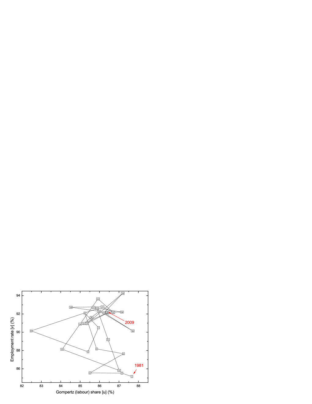
Figure 2: $[u]$-$[v]$ phase space for Brazil from 1981 to 2009. The plot points are labeled in growing numerical sequence with each integer number representing one year in the studied time interval. Thus, the label given by the number ‘1’ indicates the year 1981 and label ‘29’ means the year 2009, providing then a clear visualization of the largely clockwise evolution of the cycles. One can see that before 1995, indicated by label ‘15’, the system was cycling in a different region of the phase space. The end of hyperinflation in 1994 (label ‘14’) is possibly the event which made the system move to a new cycling region, where it still remains.

$\begin{array}[]{cc}\includegraphics[scale={0.83}]{uv-Brazil-1981-1994.eps}&\includegraphics[scale={0.70}]{uv-Brazil-1995-2009.eps}\end{array}$

Figure 3: These two graphs present the same data as in Fig. 2, but divided into two sets of points. The plot in the left shows the $[u]$-$[v]$ phase space from 1981 until 1994, whereas the right plot presents the data points from 1995 to 2009. This shows even more clearly that the Brazilian economic system moved from one region to another in the phase space during the time interval studied here. One can also note in the left plot that the system was possibly moving from yet another region in the period from 1981 to 1983, since the labels ‘1’ to ‘3’ indicating these years appear to be part of a transition from a different region than the one where the system remained until 1994. This possible interpretation has some empirical support because the high inflationary period in Brazil started in about 1980.

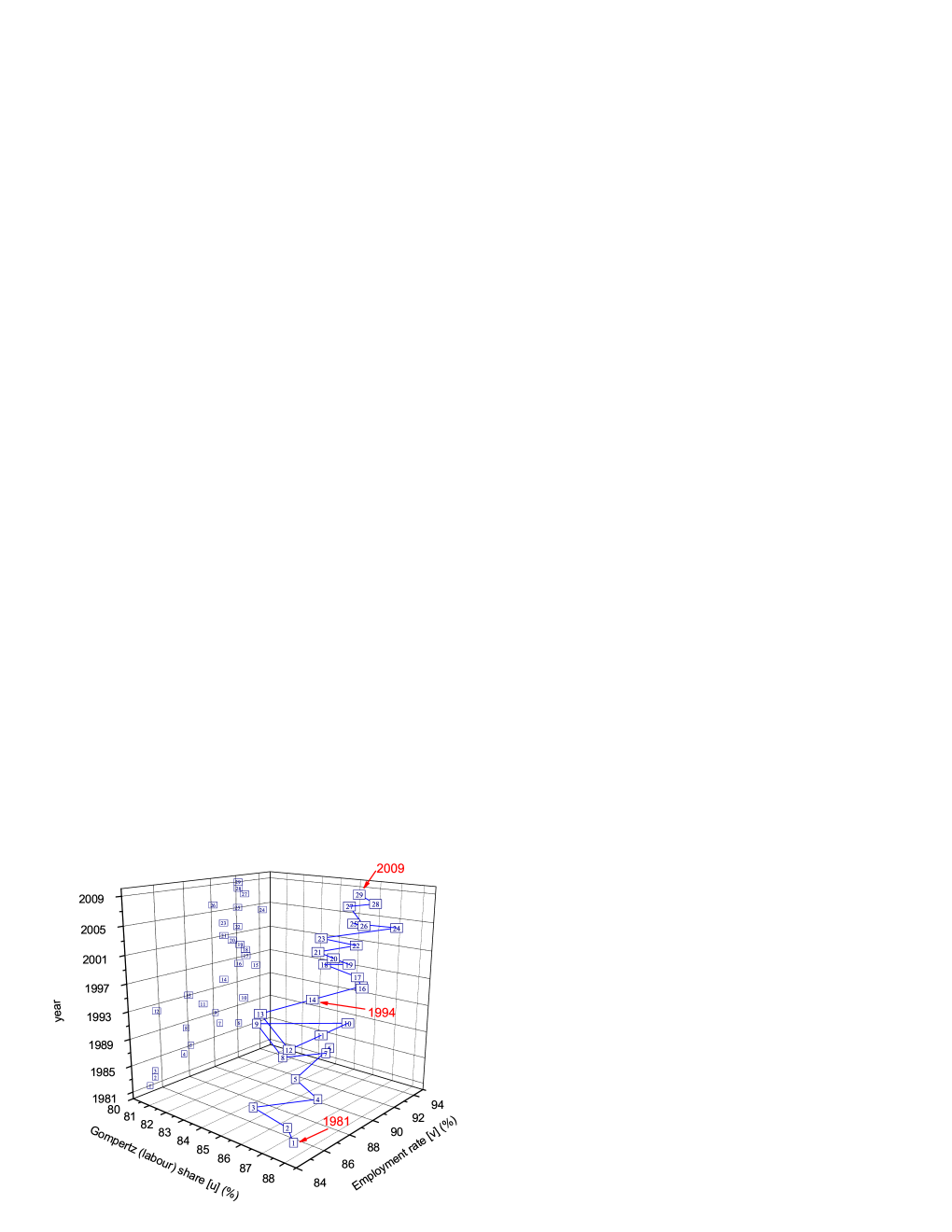
Figure 4: This plot is a 3-dimensional representation of the same points appearing in figures 2 and 3. It provides a different visualization of the system displacements during its evolution from 1981 to 2009, showing more clearly in the YZ-plane projection (the surface plane for $[v]$ vs. time, on the left side of the plot) the three regions where the system located itself in the studied time interval. The points for 1981 to 1983 (labels ‘1’ to ‘3’) seem to be a transition from an unspecified earlier region where the system stayed before the high inflationary period started at about 1980. The end of hyperinflation in 1994 (label ‘14’) moved the system to yet another region on the top right of the YZ-plane.

The important event which may explain why the apparent orbital center changes location after 1995 is the end of hyperinflation. In 1994 Brazil established a new and stable currency, the real (R$), which abruptly ended the strong inflationary period of the previous 15 years. This fact seems to be reflected in the $[u]$-$[v]$ phase space by a change in the center of the orbit. One can also see in table 1 a slow, although modest, decrease in the Gini coefficient after 1993. In addition, since the Brazilian high inflationary period started at about 1980, the positions corresponding to the years of 1981 to 1983 in the phase space appear to represent an earlier transition from yet another region in the phase space. This seems to be the case if we carefully look at these points in the graphs of figures 2 and 4.

The absence of a single center for all orbits means that the parameters $a$, $b$, $c$, $d$, and $h$ of the Goodwin model are most likely not constants at all, but time dependent variables. Nevertheless, at a qualitative level the model certainly has empirical support which justifies the identification of $[u]$ and $[v]$ with $u$ and $v$, although in order to understand the real dynamics behind these quantities one probably needs to somehow modify the dynamical equations (1) and (2) to reflect these empirical evidences.

Finally, we should note that the lack of a single orbital center in real-world data has already appeared in earlier empirical studies carried out by other authors on the Goodwin model. The $u$-$v$ phase-space plots of Desai [20], Solow [21], Harvie [22], Moreno [23], Mohun & Veneziani [24] and García Molina & Herrera Medina [25] show similar results as ours. Vadasz [10] also reached a similar conclusion, although by indirect means. The important point is that all these authors reached the same conclusion despite their use of very different methods to analyze observational data. Therefore, one feels justified to conclude that this feature appears to be universal and clearly indicate that the Goodwin model must be changed in order to accommodate this real-world feature.

5 Temporal variation of the employment rate and workers’ share

The data presented in table 1 allow us to go beyond the qualitative discussion of the previous section and carry out a quantitative evaluation of the Goodwin model and its DHMP extension. To do so we need first to carry out simple numerical estimations of the time derivative $\dot{[u]}$. This task is most straightforwardly accomplished using the following expression,

$$\dot{[u]}\approx\frac{[u](t+\Delta t)-[u](t-\Delta t)}{2\Delta t},$$ (51)

where $\Delta t=1$ year. Similar procedure is used to determine $\dot{[v]}$. The goal here is to use data fitting to estimate the parameters of the two sets of dynamical equations, the first set being given by equations (6) and (7) of the original Goodwin model and the second one by equations (12) and (13) which constitute the DHMP extension.

5.1 Goodwin model

Figure 5 shows two plots, the left one for the variables of equation (6) and the right plot for equation (7). The fitted straight lines parameter values are also presented for both plots. It is clear that both sets of points are compatible with a linear approximation similar to the original dynamical equations, but the parameters behave in exactly opposite manner from what the model predicts. While the slope of the lines predicted by equations (6) and (7) are, respectively, positive and negative, the results coming from Brazilian real-world data are the other way round. This is clear in both graphs. This result can also be seen if we use the fitted parameters to obtain conditions which the supposedly “constants” of the Goodwin model should obey. Doing so we conclude that the Brazilian economic dynamics studied here gives,

$$\left\{\begin{array}[]{ll}c<0,\\ h<0,\\ (a+d)<0,\\ (a+b)\,c>100.\end{array}\right.$$ (52)

These results completely upset the parameter conditions given by equations (3), which were thought to be valid. The fitting also leaves two parameters yet to be determined by some yet unknown equation relating them since, as seen above, the orbital center and period equations (4) are clearly invalid in the Brazilian income dynamics.

$\begin{array}[]{cc}\includegraphics[scale={0.75}]{dotu-sobre-u_vs_v.eps}&\includegraphics[scale={0.75}]{dotv-sobre-v_vs_u.eps}\end{array}$

Figure 5: Left: $\dot{[u]}/[u]$ vs. $[v]$. Right: $\dot{[v]}/[v]$ vs. $[u]$. Although both graphs show some dispersion of the results, one can clearly identify a general tendency for the observational points to decrease in the left plot and to increase in the right one. Straight line fits on both sets of results, indicated as full lines, produced the following results. For the left plot, the expression $\dot{[u]}/[u]=A_{1}+B_{1}[v]$ resulted in $A_{1}=0.17\pm 0.06$, $B_{1}=-0.0019\pm 0.0006$. For the right plot, the equation $\dot{[v]}/[v]=A_{2}+B_{2}[u]$ yielded parameters as follows: $A_{2}=-0.52\pm 0.22$, $B_{2}=0.006\pm 0.003$. These results should be compared with equations (6) and (7).

The calculated uncertainties in the fitted parameters do not change this situation, a fact which forces us to conclude that the economic hypotheses advanced by Goodwin to derive his model are either not applicable, partially or completely, to the economic system studied here or they are flawed. Whatever conclusion one may choose, this analysis indicates that to advance this model with the aim of turning it into a viable representation of the real world, the focus must lie on the probable modification of the set of differential equations (6) and (7) and their empirical validation, rather than how they were obtained. Only after a good model is achieved, and by good we mean a model with solid empirical foundations, may we start looking for the real economic conditions behind its dynamics.

Since the data show that the parameters of the model follow the exact opposite predictions given by the expressions (3), another consequence of the results shown in figure 5 is the reversal of the predicted roles of predator and prey discussed in Sect. 2.1. Indeed, according to the fitted parameters (see caption of figure 5), when $[u]=0$, $\dot{[u]}=0$ and $\dot{[v]}<0$. In this case $[u]$ plays the role of prey because without it ($[u]=0$) the predator population decreases ($\dot{[v]}<0$). Similarly, when $v=0$, $\dot{[v]}=0$ and $\dot{[u]}>0$. So, $v$ plays the role of predator because without them ($v=0$) the prey population grows without bounds ($\dot{[u]}>0$). Such a reversal of roles of predators and preys coming from the real-world data analysis presented here also implies a reversal of the reasoning presented in Sect. 2.3 regarding how one interprets the conflicting variables. However, although such role discussions had some importance in the past, such interpretations are now of lesser importance than revealing the inner dynamics of these two inter-dependent variables. When such dynamics is better understood by means of realistic, not introspective, models, such roles will naturally emerge from those real-world representations.

5.2 DHMP extension

The variables in the dynamical equations (12) and (13) of the DHMP extension are plotted in figure 6. To do so we had to choose a value for the maximum share of labor $\bar{[u]}$. From table 1 we see that the highest value in the studied time period is 87.7% in 1981 and in view of the fact that the DHMP model does not give any hint about how to obtain $\bar{[u]}$, assuming whatever constant value higher than that is enough for our purposes here and will not change the general behavior of equation (13). So, we chose $\bar{[u]}=95\%$ as a reasonable value for this analysis.

The left plot in figure 6 shows the points related to the dynamical variables of equation (12) while the right graph in concerned with the variables appearing in equation (13). The fitted parameters are written in the figure caption and, similarly to our reasoning above, they produce real-world conditions for the “constants” of the DHMP model. They may be written as follows,

$$\left\{\begin{array}[]{ll}\delta>0\;\;(?),\\ \bar{h}>0\;\;(?),\\ (\bar{a}+\bar{d})>0\;\;(?),\\ \lambda<0,\\ (\bar{a}+\bar{b})<-\lambda\ln(100-\bar{u}).\\ \end{array}\right.$$ (53)

The results with a question mark are inconclusive due to the uncertainties of the fitted parameters. For the other two, $\lambda<0$ contradicts the prediction given in equations (10), but implies that $(\bar{a}+\bar{b})>0$ for the chosen $\bar{u}$. So, despite the fitting, the DHMP model remains in a very inconclusive status regarding the empirical behavior of its dynamical variables and its supposedly constant parameters. Even so, because the model has too many parameters, after a successful fitting where one of the parameters had to be assumed ($\bar{u}$), two other parameters remained unknown and still require determination by at least another, also unknown, expression.

In conclusion, because the DHMP extension has more unknown quantities and its dynamics is described by somewhat more complex differential equations than the original Goodwin model, comparing its predictions with the Brazilian data renders mixed and inconclusive results. Adding to this situation are the high errors in the fitted parameters and the fact that even after a successful fit several parameters remain unknown. These results place the DHMP extension in a much less favorable situation than the original Goodwin model regarding empirical validity, at least as far as Brazilian data is concerned.

$\begin{array}[]{cc}\includegraphics[scale={0.75}]{dotu-sobre-u_vs_Vgrande-eq12.eps}&\includegraphics[scale={0.75}]{dotv-sobre-v_vs_ln95-u_eq13.eps}\end{array}$

Figure 6: Left: $\dot{[u]}/[u]$ vs. $[V]$. Right: $\dot{[v]}/[v]$ vs. $[\mathcal{U}]$ (see equations 14 and 15), where $\bar{u}$ was assumed as 95%. In the left plot the full line indicates a power-law fit of the form $\dot{[u]}/[u]=\bar{A}_{1}+\bar{B}_{1}[V]^{\bar{\delta}}$. The fitting parameters yielded $\bar{A}_{1}=-0.011\pm 0.022$, $\bar{B}_{1}=0.0003\pm 0.0027$ and $\bar{\delta}=1.59\pm 2.94$, results which should be compared with equation (12). For the right graph the full line indicates a straight line fit using the expression $\dot{[v]}/[v]=\bar{A}_{2}+\bar{B}_{2}\ln(95-[u])$. The resulting fitted parameters are $\bar{A}_{2}=0.12\pm 0.05$ and $\bar{B}_{2}=-0.054\pm 0.024$. This result should be compared with equation (13).

6 Conclusions

In this paper we have studied the empirical validity of the model of economic growth with cycles advanced by Goodwin [2, 3] and one of its specific variations, the Desai-Henry-Mosley-Pemberton (DHMP) extension [9], using Brazilian income data from 1981 to 2009. The variables used by Goodwin in his model, the workers’ share of total production $u$ and employment rate $v$ were obtained by describing the individual income distribution by the Gompertz-Pareto distribution (GPD) [27], formed by the combination of the Gompertz curve, representing the overwhelming majority of the population ($\sim\,$99%), with the Pareto power law, representing the tiny richest part ($\sim\,$1%) [26]. We identified the Gompertzian part of the distribution with the workers and the Paretian component with the class of capitalists and used GPD parameters obtained for each year in the studied time period to analyze the time evolution of these variables by means of the Goodwin dynamics. Unemployment data was also obtained from income distribution so that all variables come from the same sample since Brazilian unemployment data was collected under different methodologies during the time span analyzed here.

The results were, however, mixed, both qualitatively and quantitatively. The data showed clockwise cycles in the $u$-$v$ phase space in agreement with the model, but those cycles were only largely clockwise and the orbital center was not unique, results which brought only partial qualitative agreement of the model with Brazilian data. We obtained temporal variations of the variables and their derivatives and carried out straight line fittings to the points formed with these quantities, both in the original Goodwin model and its DHMP extension in order to obtain fitting parameters which were compared with predictions of both models. In this respect the original model was able to provide a better empirical consistency, but the observed parameters were different from what the model predicts in the sense of their general behavior, leading to fitted lines whose slopes had opposite behavior than the theory states. A similar situation occurred with the DHMP extension, but in this case the uncertainties in the fitted parameters were too large, leading to mostly inconclusive results. Although a general predator-prey like behavior was observed, the lack of a single orbital center and parameters behaving very differently from what was anticipated bring into question the economic hypotheses used by Goodwin in deriving his model. It appears that they may be inapplicable to the economic system under study, a conclusion which comes as no surprise in view of the extremely simple specifications of the model, as discussed in Sect. 2.4.

Considering these results, in order to provide a viable representation of the real world the Goodwin model must be modified. Firstly, as it is obvious from our results, as well as the ones obtained by previous authors, there cannot be a single orbital center. We can envisage two possible reasons for such a result: (i) the “constants” of the model may not be constants at all, but time variables; (ii) the right-hand side of equations (6) and (7) are too simple and may require more terms involving the two variables, which means giving up the linear approximation of equations (23) and (29). In other words, going to a fully nonlinear modeling.

Secondly, the emphasis so far given by several studies on the economic foundations of the model, which have been the main source for its proposed theoretical modifications, should be put aside, at least temporarily, in favor of devising differential equations capable of reproducing the observed features, like the moving orbital centers and the behavior of the graphs with the temporal variations of $u$ and $v$. Clearly those economic hypotheses will need to be revised as they produce a model which does not agree with the data, but these revisions must be made in the light of empirical results and not solely by theoretical introspection. Possibly new variables representing other economic players, like debt and government policy, may have to be introduced in the model, which means that, perhaps, more than two coupled differential equations would be necessary to define the economic system. In this respect, as discussed by Keen [18], Hudson [41] and Hudson & Bezemer [42], investment is not profit, being debt-financed when it exceeds profit, and government taxation has to be deduced from output to determine profit.

Thirdly, since the DHMP model fared much more poorly as compared to the original model, Occam’s razor dictates that these modifications must be focused in the latter rather than the former because the original model is simpler. So, developing more complex models without a clear empirical motivation, and in the absence of a clear guidance given by real-data observations, goes against Occam’s razor.

The basic motivation behind these proposed modifications comes from the realization that in its present state the Goodwin model does not provide much more explanatory power beyond the original qualitative ideas advanced by Marx. This is so because it is essentially a mathematical dressing of Marxian ideas by means of a predator-prey set of first order differential equations, but which produces solutions that clearly contradict empirical data in many respects and provides only general qualitative agreement with real-world observations. Therefore, the real challenge lies in devising a model that addresses real-world data and is capable of surviving empirical verification. One must always keep in mind that the good scientific practice entails a permanent search of convergence between hypotheses and evidences.

Our thanks go to E. Screpanti for the initial encouragement to pursue this research, S. Sordi for pointing out relevant bibliographic information at the beginning of this project and M. Desai and A. Kirman for discussions. We are also grateful to S. Keen for various very interesting and useful insights on the origins of the Goodwin model and the referees for useful comments. One of us (MBR) acknowledges partial financial support from the Rio de Janeiro State funding agency FAPERJ.

References

- [1] K. Marx, “Capital”, vol. I, book one (1867, 1st German ed.); Marx/Engels Internet Archive (1st English ed., 1887): http://www.marxists.org/archive/marx/works/1867-c1/. Accessed 14 August 2012
- [2] R.M. Goodwin, “A Growth Cycle”. In “Socialism, Capitalism and Economics”, ed. C.H. Feinstein, (Cambridge University Press, 1967), pp. 54-58. See also “The History of Economic Thought Website”, http://cruel.org/econthought/essays/multacc/goodw2.html. Accessed 4 September 2012
- [3] G. Gandolfo, “Economic Dynamics”, (Springer: Berlin, 1997)
- [4] R.M. Goodwin, “Disaggregating Models of Fluctuating Growth”. In “Nonlinear Models of Fluctuations and Growth”, ed. R.M. Goodwin, M. Krüger & A. Vercelli, (Springer: Berlin, 1984), pp. 67-72
- [5] M.C. Sportelli, “A Kolmogoroff Generalized Predator-Prey Model of Goodwin’s Growth Cycle”, J. Econ. 61 (1995) 35-64
- [6] S. Sordi, “Economic Models and the Relevance of ‘Chaotic Regions’: An Application to Goodwin’s Growth Cycle Model”, Annals Op. Research 89 (1999) 3-21
- [7] S. Sordi, “Growth Cycles When Workers Save. A Reformulation of Goodwin’s Model along Kaldorian-Pasinettian Lines”, Central Eur. J. Op. Research 9 (2001) 97-117
- [8] R. Veneziani, “Structural Stability and Goodwin’s ‘A Growth Cycle.’ A survey”, (2001) Ente per gli studi monetari, bancari e finanziari “Luigi Einaudi.” Temi di ricerca (24), http://www.enteluigieinaudi.it/pdf/Pubblicazioni/Temi/T_24.pdf. Accessed 14 August 2012
- [9] M. Desai, B. Henry, A. Mosley & M. Pemberton, “A Clarification of the Goodwin Model of the Growth Cycle”, J. Econ. Dyn. Control 30 (2006) 2661-2670
- [10] V. Vadasz, “Economic Motion: An Application of the Lotka-Volterra Equations”, Undergraduate Honors Thesis, (Franklin and Marshall College Archives, 2007), http://dspace.nitle.org/handle/10090/4287. Accessed 14 August 2012
- [11] R. Veneziani & S. Mohun, “Structural Stability and Goodwin’s Growth Cycle”, Struc. Ch. Econ. Dyn. 17 (2006) 437-451
- [12] G. Dibeh, D.G. Luchinsky, D.D. Luchinskaya & V.N. Smelyanskiy, “A Bayesian Estimation of a Stochastic Predator-Prey Model of Economic Fluctuations”. In “Noise and Stochastics in Complex Systems and Finance”, ed. J. Kertész, S. Bornholdt & R.N. Mantegna: Proc. SPIE Vol. 6601 (2007) 660115
- [13] J. Kodera & M. Vosvrda, “Goodwin’s Predator-Prey Model with Endogenous Technological Progress”, IES Working Paper 9/2007, (Charles University, 2007), http://ideas.repec.org/p/fau/wpaper/wp2007_09.html. Accessed 14 August 2012
- [14] G. Colacchio, M. Sparro & C. Tebaldi, “Sequences of Cycles and Transitions to Chaos in a Modified Goodwin’s Growth Cycle Model”, Int. J. Bif. Chaos 17 (2007) 1911-1932
- [15] C. Tebaldi & G. Colacchio, “Chaotic Behavior in a Modified Goodwin’s Growth Cycle Model”. In “Proceedings of the 2007 International Conference of the System Dynamics Society”, pp. 0-20, (The System Dynamics Society, 2007)
- [16] L. Aguiar-Conraria, “A Note on the Stability Properties of Goodwin’s Predator-Prey Model”, Rev. Rad. Pol. Econ., 40 (2008) 518
- [17] A. Bródy & I. Ábel, “Amends of an Old Feud (Goodwin’s Flair for the Law of Conservation)”, Acta Oeconomica 60 (2010) 127-141
- [18] S. Keen, “Finance and Economic Breakdown: Modelling Minsky’s ‘Financial Instability Hypothesis’ ”, J. Post Keynesian Economics 17 (1995) 607-635
- [19] A.B. Atkinson, “The Timescale of Economic Models: How Long is the Long Run?”, Rev. Econ. Studies 36 (1969) 137-152
- [20] M. Desai, “An Econometric Model of the Share of Wages in National Income: UK 1855-1965”. In “Nonlinear Models of Fluctuations and Growth”, ed. R.M. Goodwin, M. Krüger & A. Vercelli, (Springer: Berlin, 1984), pp. 24-27
- [21] R. Solow, “Goodwin’s Growth Cycle: Reminiscence and Rumination”. In “Nonlinear and Multisectoral Macro-dynamics: Essays in Honour of Richard Goodwin”, ed. K. Velupillai, (Macmillan: London, 1990), pp. 31-41
- [22] D. Harvie, “Testing Goodwin: Growth Cycles in Ten OECD Countries”, Cambridge J. Econ. 24 (2000) 349-376
- [23] A.M. Moreno R., “El Modelo de Ciclo y Crecimiento de Richard Goodwin. Una Evaluación Empírica para Colombia”, Cuadernos de Economía, 21, Nr. 37 (2002) 1-20
- [24] S. Mohun & R. Veneziani, “Goodwin Cycles and the U.S. Economy, 1948-2004”, preprint (2006), Munich Personal RePEc Archive (MPRA) paper No. 30444, http://mpra.ub.uni-muenchen.de/30444
- [25] M. García Molina & E. Herrera Medina, “Are There Goodwin Employment-Distribution Cycles? International Empirical Evidence”, Cuadernos de Economía, 29, Nr. 53 (2010) 1-29
- [26] N.J. Moura Jr. & M.B. Ribeiro, “Evidence for the Gompertz Curve in the Income Distribution of Brazil 1978-2005”, Eur. Phys. J. B, 67 (2009) 101-120, arXiv:0812.2664v1
- [27] F. Chami Figueira, N.J. Moura Jr. & M.B. Ribeiro, “The Gompertz-Pareto Income Distribution”, Physica A, 390 (2011) 689-698, arXiv:1010.1994v1
- [28] S. Keen, private communication (2012)
- [29] R. Solow, “Building a Science of Economics for the Real World”, Prepared Statement to the House Committee on Science and Technology, Subcommittee on Investigations and Oversight (20 July 2010), http://www2.econ.iastate.edu/classes/econ502/tesfatsion/Solow.StateOfMacro.CongressionalTestimony.July2010.pdf. Accessed 12 September 2012
- [30] W. Buiter, “The Unfortunate Uselessness of Most ‘State of the Art’ Academic Monetary Economics”, Financial Times (3 March 2009), http://blogs.ft.com/maverecon/2009/03/the-unfortunate-uselessness-of-most-state-of-the-art-academic-monetary-economics/. Accessed 10 August 2012
- [31] P. Mirowski, “The Seekers, or How Mainstream Economists Have Defended their Discipline since 2008”, Part I: “Them Crazy Seekers”, Part II: “Behavioural Economics - Rationalising Irrationality”, Part III: “Microirrationalities - a Critic’s Defence of the System”, Part V. “DSGE and the Threatened Unravelling of the Whole Damnn Thing”, (December 2011), http://www.nakedcapitalism.com. Accessed 31 October 2012
- [32] A. Kirman, “Economic Theory and the Crisis”, Real-World Economics Review, Nr. 51 (2009) 80-83
- [33] S. Keen, “Mad, Bad and Dangerous to Know”, Real-World Economics Review, Nr. 49 (2009) 2-7
- [34] S. Keen, “1,000,000 economists can be wrong: the free trade fallacies”, (30 September 2011), http://www.debtdeflation.com/blogs/2011/09/30/1000000-economists-can-be-wrong-the-free-trade-fallacies/. Accessed 24 September 2012
- [35] D. Colander, M. Goldberg, A. Haas, K. Juselius, A. Kirman, T. Lux & B. Sloth, “The Financial Crisis and the Systemic Failure of Economics Profession”, Critical Review, 21 (2009) 249-267; earlier version (with Hans Fölmer), “The Financial Crisis and the Systemic Failure of Academic Economics”, Kiel Institute Working Paper Nr. 1489 (February 2009), http://ideas.repec.org/p/kie/kieliw/1489.html. Accessed 14 August 2012
- [36] Memorandum of German-Speaking World Economics Professors, “Towards a Renewal of Economics as a Social Science”, World Economics Association Newsletter, 2, Nr. 3 (June 2012) 6-7
- [37] P. Krugman, “How did Economists Get it so Wrong?”, New York Times, (2 September 2009), http://www.nytimes.com/2009/09/06/magazine/06Economic-t.html. Accessed 12 September 2012
- [38] R. Johnson, “Economists: a Profession at Sea”, Time Magazine (19 January 2012), http://business.time.com/2012/01/19/economists-a-profession-at-sea. Accessed 3 September 2012
- [39] J. T. Harvey, “How Economists Contributed to the Financial Crisis”, Forbes (6 February 2012), http://www.forbes.com/sites/johntharvey/2012/02/06/economics-crisis/. Accessed 16 September 2012
- [40] P. Soos, “Stop letting economists off the hook”, Business Spectator (16 March 2012), http://www.businessspectator.com.au/bs.nsf/Article/economists-wrong-calls-financial-crisis-pd20120315-SDW4X. Accessed 24 October 2012
- [41] M. Hudson, “The Bubble and Beyond”, (Islet-Verlag: Dresden, 2012)
- [42] M. Hudson & D. Bezemer, “Incorporating the Rentier Sectors into a Financial Model”, World Economic Review, 1 (2012) 1-12
- [43] J. Doyne Farmer, Martin Shubik, Eric Smith, “Is Economics the Next Physical Science?”, Physics Today (September 2005) 37-42
- [44] C. Schinckus, “Econophysics and Economics: Sister Disciplines?”, Am. J. Phys., 78 (2010) 325-327
- [45] C. Schinckus, “Is Econophysics a New Discipline? The Neopositivist Argument”, Physica A, 389 (2010) 3814-3821
- [46] M. B. Ribeiro & A. A. P. Videira, “Dogmatism and Theoretical Pluralism in Modern Cosmology”, Apeiron, 5 (1998) 227-234, arXiv:physics/9806011v1
- [47] T. Lawson, “Mathematical Modelling and Ideology in the Economics Academy: Competing Explanations of the Failings of the Modern Discipline?”, Economic Thought, 1 (2012) 3-22
- [48] M. Hudson, “The Use and Abuse of Mathematical Economics”, Real-World Economics Review, Nr. 55 (2010) 2-22
- [49] M.B. Ribeiro & A.A.P. Videira, “Boltzmann’s Concept of Reality”, preprint (2007), arXiv:physics/0701308v1
- [50] L. Boltzmann, “On the Fundamental Principles and Equations of Mechanics”, Populäre Schriften, Essay 16 (1899). In “Theoretical Physics and Philosophical Problems”, English edition by B. McGuinness, (Reidel: Dordrecht, 1974), pp. 101-128
- [51] J.P. Bouchaud, “Economics Needs a Scientific Revolution”, Nature, 455 (2008) 1181; Real-World Economics Review, Nr. 48 (2008) 291-292, arXiv:0810.5306v1
- [52] J.P. Bouchaud, “The (Unfortunate) Complexity of the Economy”, Physics World (April 2009) 28-32, arXiv:0904.0805v1
- [53] S. Sinha, A. Chatterjee, A. Chakraborti & B.K. Chakrabarti, “Econophysics”, (Wiley-VCH Verlag: Weinheim, 2011)
- [54] D. Calderwood, “Cargo Cult Economics”, (2008), http://www.lewrockwell.com/calderwood/calderwood24.html; Political Calculations (2009), http://politicalcalculations.blogspot.com.br/2009/03/economics-needs-scientific-revolution.html. Accessed 10 August 2012.
- [55] R. P. Feynman, “Cargo Cult Science”, Engineering and Science (June 1974) 10-13
- [56] T. M. Georges, “Cargo Cult Science - Revisited”, (2008), http://tgeorges.home.comcast.net/~tgeorges/cargo.htm. Accessed 10 August 2012
- [57] S. Birks, “Why Pluralism?”, World Economics Association Newsletter, 1, Nr. 1 (December 2011), 2
- [58] A. Kirman (interview), Non-Equilibrium Social Science Newsletter, Nr. 4 (May 2012) 2-8