The Atacama Cosmology Telescope: Temperature and Gravitational Lensing Power Spectrum Measurements from Three Seasons of Data

Abstract

We present the temperature power spectra of the cosmic microwave background (CMB) derived from the three seasons of data from the Atacama Cosmology Telescope (ACT) at 148 GHz and 218 GHz, as well as the cross-frequency spectrum between the two channels. We detect and correct for contamination due to the Galactic cirrus in our equatorial maps. We present the results of a number of tests for possible systematic error and conclude that any effects are not significant compared to the statistical errors we quote. Where they overlap, we cross-correlate the ACT and the South Pole Telescope (SPT) maps and show they are consistent. The measurements of higher-order peaks in the CMB power spectrum provide an additional test of the $\Lambda$CDM cosmological model, and help constrain extensions beyond the standard model. The small angular scale power spectrum also provides constraining power on the Sunyaev-Zel’dovich effects and extragalactic foregrounds. We also present a measurement of the CMB gravitational lensing convergence power spectrum at $4.6\sigma$ detection significance.

1. INTRODUCTION

The current generation of arcminute resolution cosmic microwave background (CMB) experiments is providing researchers with a precise view of CMB anisotropies over a range of scales ($500<\ell<10000$). Over the so-called Silk damping tail of the CMB ($500<\ell<3000$) these observations are revealing the subtle effects that inflationary physics, primordial helium density and the energy density in relativistic degrees of freedom have on the acoustic oscillations in the photon-baryon plasma in the radiation-dominated era. Rapid progress in measurements of the damping tail of the power spectrum has been achieved over a span of a few years by a number of experiments, notably the Cosmic Background Imager (CBI; Sievers et al. 2009), Arcminute Cosmology Bolometer Array Receiver (ACBAR; Reichardt et al. 2009), QUEST at DASI (QUaD; Brown et al. 2009; Friedman et al. 2009), the Atacama Cosmology Telescope (ACT; Swetz et al. 2010; Fowler et al. 2010; Das et al. 2011b, hereafter D11; Dunkley et al. 2011) and the South Pole Telescope (SPT; Keisler et al. 2011; Story et al. 2012).

Figure 1.— Equatorial maps (ACT-E) made from 2009 (upper panel) and 2010 (lower panel) 148 GHz observations filtered to emphasize modes in the range $\ell=500-2500$. The four data splits in either season were co-added to make this plot. Also delineated are the patches used for computing power spectra.

Minute distortions of the CMB anisotropies due to the gravitational lensing of CMB photons by large-scale structure have now been detected using CMB data alone, both in percent-level alteration of the damping tail acoustic peak structure (D11, Keisler et al. 2011, Story et al. 2012), and in the subtle non-Gaussian signature it induces in the statistics of CMB anisotropies (Das et al., 2011a; van Engelen et al., 2012). When added to the cosmic variance-limited CMB power spectrum measurements at $\ell\lesssim 1000$ by the WMAP satellite (Larson et al., 2011), the damping tail measurements are providing additional dynamic range resulting in improved constraints on inflationary parameters such as the tilt and running of the primordial power spectrum. On smaller scales ($\ell>3000$) the primordial CMB signal diminishes and emission from radio galaxies and dusty star forming galaxies, as well as the thermal and kinematic Sunyaev-Zel’dovich effects (Sunyaev & Zeldovich, 1972) arising from the scattering of CMB photons by hot gas in galaxy clusters, dominate the power spectrum. Along with the damping tail measurements, rapid progress has been made in the measurements and modeling of this high-multipole tail (Lueker et al. 2010; Shirokoff et al. 2011; D11; Dunkley et al. 2011, Reichardt et al. 2012). These measurements have been used to estimate the thermal and kinematic SZ contributions to the power spectrum, as well as to model the cosmic infrared background (CIB) power spectrum arising from the mm-wave emission from dusty high redshift galaxies (Hall et al., 2010; Dunkley et al., 2011; Addison et al., 2012b, a; Hajian et al., 2012; Reichardt et al., 2012; Zahn et al., 2012).

In this work, we present the measurement of the power spectra of CMB temperature anisotropies at 148 GHz and 218 GHz from a subset of ACT observations performed over the 2008, 2009 and 2010 observing seasons, and covering approximately 600 deg² of the sky. This is approximately twice the survey area used in a previous measurement of the ACT power spectrum(D11). Additionally, we also present an updated measurement of the gravitational lensing power spectrum from the equatorial strip. Dunkley et al. (2013) use the temperature bandpowers reported in this work to generate likelihood functions which form the basis of the cosmological parameter constraints reported by Sievers et al. (2012).

The paper is organized as follows. In Section 2 we describe the observations, the generation of maps from time ordered data, and the estimation of the beam transfer functions. We discuss the calibration of the maps in Section 3. Section 4 describes the pipeline used to process the maps into the angular power spectrum. Treatment of point sources and other foregrounds is discussed in Section 5. Simulations used to test and validate various portions of the power spectrum estimation pipeline are described in Section 6. The power spectrum results and consistency checks are presented in Section 7, and the CMB lensing results are discussed in Section 8. We conclude in Section 9.

2. OBSERVATIONS AND FIELDS

ACT is a 6-meter off-axis Gregorian telescope situated in the Atacama desert in Chile at an elevation of 5190 m. ACT’s Millimeter Bolometric Array Camera (MBAC) has three channels operating at 148 GHz, 218 GHz and 277 GHz. The instrument is described in detail in Swetz et al. (2011). Between 2007 and 2010 ACT observed mainly along two constant-declination strips on the sky: one running along the celestial equator (hereafter the equatorial strip or ACT-E), and the other along declination -55 ° in the southern sky (the southern strip or ACT-S). The observations were performed over Nov 8 – Dec 15, 2007; Aug 11 – Dec 24, 2008; May 18 – Dec 18, 2009, and Apr 6 – Dec 27, 2010. Here we present the angular power spectrum measurements of 148 GHz and 218 GHz observations from 300 deg² on ACT-E and 292 deg² on ACT-S. Table 1 summarizes the observations from various seasons that were used in estimating the power spectrum, and also defines shorthand notations for maps, e.g., the 2009 season equatorial map is referred to as the “season 3e” or simply the “3e” map.

Table 1Observations used in power spectrum estimation

Year	Key	R.A. Range	Dec. Range	Area	$n_{p}$
				(deg2)
Equatorial Strip ACT-E
2009	3e	${20}^{\mathrm{h}}{40}^{\mathrm{m}}$ .. ${3}^{\mathrm{h}}{20}^{\mathrm{m}}$	-1$.\!\!^{\circ}$5 .. 1$.\!\!^{\circ}$5	300	5
2010	4e	${20}^{\mathrm{h}}{40}^{\mathrm{m}}$ .. ${3}^{\mathrm{h}}{20}^{\mathrm{m}}$	-1$.\!\!^{\circ}$5 .. 1$.\!\!^{\circ}$5	300	5
Southern Strip ACT-S
2008f	2sf	${00}^{\mathrm{h}}{22}^{\mathrm{m}}$ .. ${06}^{\mathrm{h}}{47}^{\mathrm{m}}$	-55$.\!\!^{\circ}$0 .. -50$.\!\!^{\circ}$0	292	4
2008	2s	${04}^{\mathrm{h}}{08}^{\mathrm{m}}$ .. ${07}^{\mathrm{h}}{08}^{\mathrm{m}}$	-55$.\!\!^{\circ}$2 .. -51$.\!\!^{\circ}$2	146	2
2009	3s	${04}^{\mathrm{h}}{08}^{\mathrm{m}}$ .. ${07}^{\mathrm{h}}{08}^{\mathrm{m}}$	-55$.\!\!^{\circ}$2 .. -51$.\!\!^{\circ}$2	146	2
2010	4s	${04}^{\mathrm{h}}{08}^{\mathrm{m}}$ .. ${07}^{\mathrm{h}}{08}^{\mathrm{m}}$	-55$.\!\!^{\circ}$2 .. -51$.\!\!^{\circ}$2	146	2

2.1. Equatorial Observations

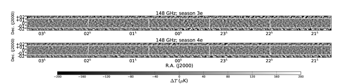
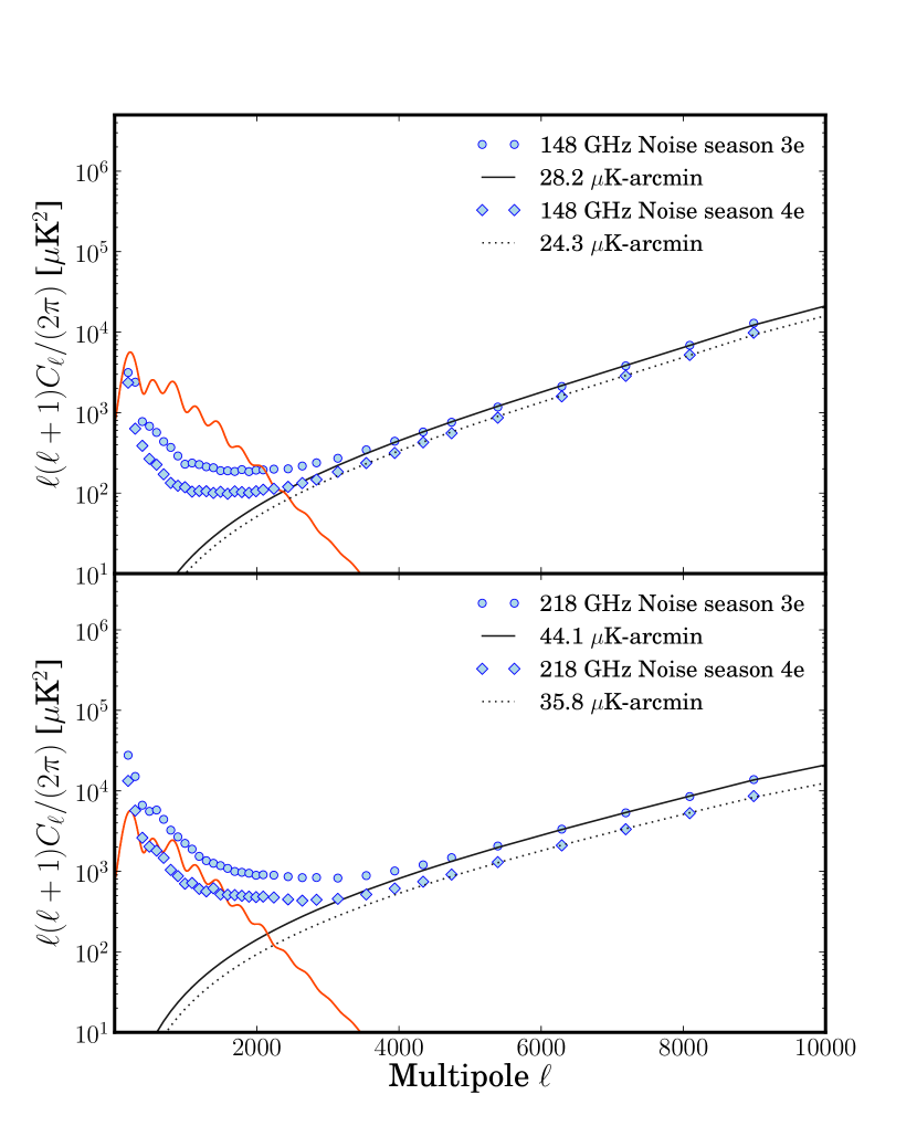
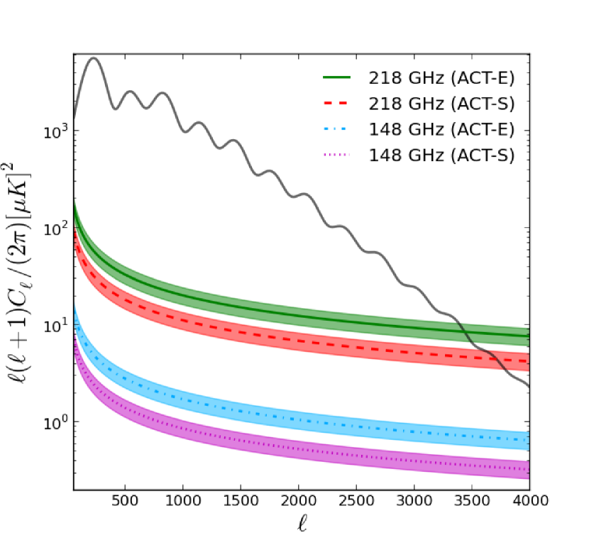
Observations on the ACT-E strip were performed in the 2009 and 2010 seasons, and run along the celestial equator with a right ascension span of 100 degrees, and a width of 3 degrees along the declination direction. For the power spectrum analysis, we make single season maps, and following D11 we divide the data within each season into four splits in time, by distributing data from roughly every fourth night into a different split, generating four split-maps, each of which is properly cross-linked. The maps are also spatially divided into five patches on which power spectrum estimation is performed separately. We explicitly avoid the edges of the maps where the cross-linking is poor and the noise is inhomogeneous. A representation of the season 3e and season 4e 148 GHz maps and patches are shown in Fig. 1. The two seasons share the same footprint on the sky, and common patches were defined to facilitate the computation of cross season power spectra. Fig. 2 shows the noise power spectra of the ACT-E maps by season against the CMB-only theory. For most seasons, and for 148 GHz, on largest angular scales ($\ell<500$) atmospheric noise dominates, while for intermediate angular scales ($500<\ell<2500$) fluctuations in the CMB dominate the variance. At smaller angular scales detector noise becomes the most significant contribution.

Figure 2.— Noise spectra for each season for the ACT-E maps for 148 GHz (upper panel) and 218 GHz (lower panel). The red solid line shows the CMB-only spectrum. At 148 GHz the power spectrum is sample variance limited at $\ell<2500$, while at 218 GHz detector and atmospheric noise dominate on most scales.

2.2. Southern Observations

Figure 3.— Southern maps (ACT-S) made from 2008 (top panel) 2009 (middle panel) and 2010 (bottom panel) 148 GHz  observations filtered to emphasize modes in the range $\ell=500-2500$. The four data splits were co-added to make this plot. Also delineated are the patches used for computing power spectra. The smaller two patches common between the three maps are used to compute cross-season cross-power spectra. The four larger patches for season 2sf are used to compute the full footprint 2008-only cross-power spectrum. Areas of large noise or stripes are heavily down weighted in the analysis. The color scale is the same as Fig 1.

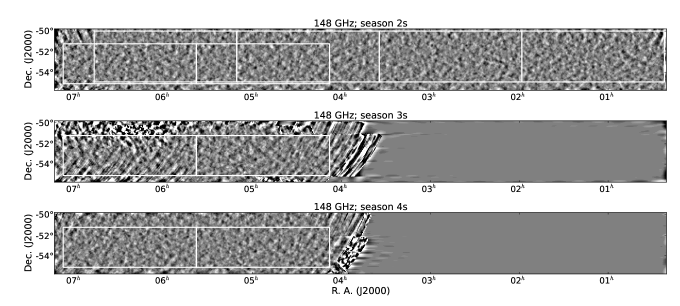
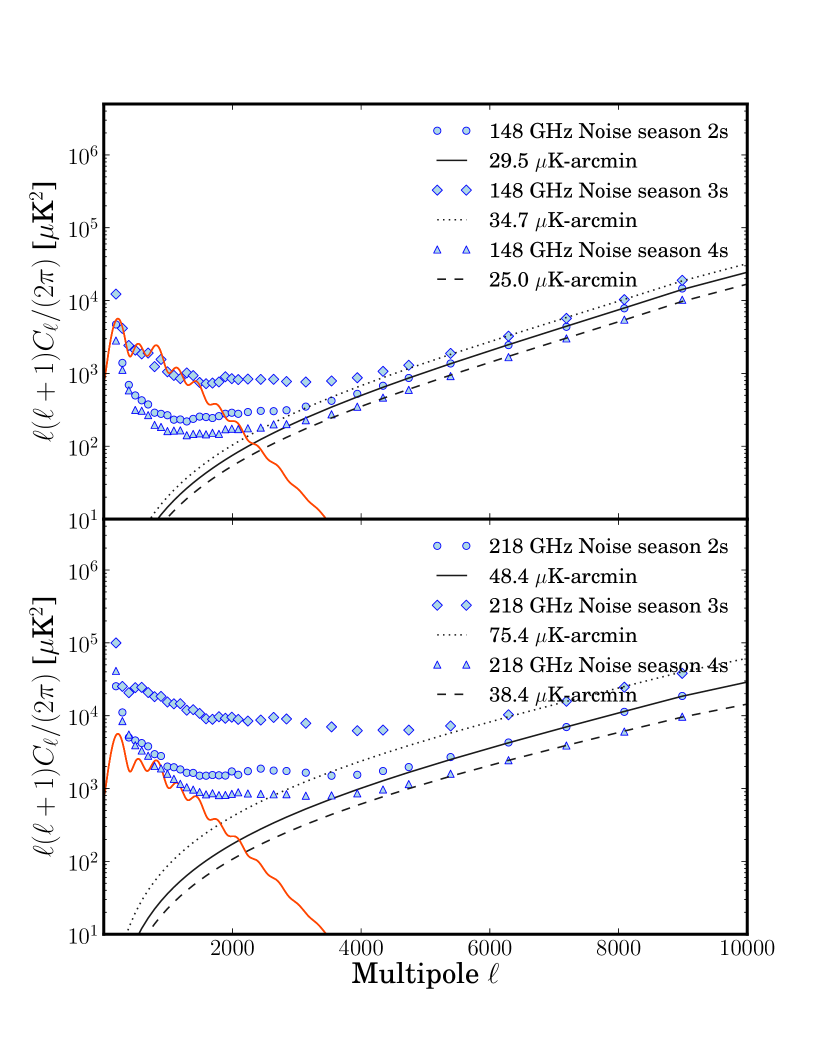
The observations made on the southern sky across various seasons had different footprints, requiring a somewhat involved strategy for efficiently computing the power spectrum. Filtered versions of various season maps are shown in Fig. 3. The largest coverage was obtained in the 2008 season (the same area on which D11 was based). When computing the power spectrum within the 2008 data set, we used four large patches collectively covering 292 deg² (we refer to this full footprint as “season 2 south full” or season 2sf in short). For computing the power spectrum within the other two seasons, as well as to compute the cross-power spectra between any pair of the three seasons it was necessary to define another set of two patches (shown by the smaller contiguous rectangles in Fig. 3) that had a common footprint across the seasons. As discussed in Section 4, care was taken not to double count information while combining the different spectra. The noise power spectra of each of the season maps are displayed in Fig. 4 against the CMB-only theory. The season 3s map is mostly noise dominated on all scales in either frequency – we keep this season in our analysis to tease out information from cross-season spectra, but the season 3s-only spectrum is heavily downweighted in our likelihood.

Figure 4.— Noise spectra for each seasons for the ACT-S maps for 148 GHz (upper panel) an 218 GHz (lower panel). The red solid line shows the CMB-only spectrum. Season 3s is significantly noisier than the other two seasons. Note that the combination of seasons 3s and 4s is more sensitive than season 2s which was used in D11 and Dunkley et al. (2011).

2.3. From Time-Ordered Data to Maps

Figure 5.— Comparison of a sky patch from the WMAP 7-year 94 GHz map (Jarosik et al., 2011) (top) with the map of the same region made from ACT 148 GHz (bottom) observations (co-added across seasons). All maps have been high-pass filtered with a $\cos^{2}\ell$-like filter that goes from 0 to 1 for $100<\ell<300$. Agreement between the CMB features in the two maps is clear by eye.

Figure 6.— Side by side comparison between the ACT map (co-added across seasons) and the SPT map for the same region of the sky. The left panel shows the ACT map high-pass filtered with a $\cos^{2}\ell$-like filter that goes from 0 to 1 for $100<\ell<300$, and the center and right panels show the ACT and SPT maps respectively under the same high-pass filter used in the SPT data release (Schaffer et al., 2011). Agreement between the CMB features in the two maps is clear by eye. It is noteworthy that the instrumentation, scan strategy, and analysis methods for these two experiments are completely different.

Details of the map-making procedure starting from time-ordered data can be found in Dünner et al. (2012). The maps were produced using the algorithm described in Dünner et al. (2012), and the 148 GHz 2008 data are identical to the maps presented there. We present a short summary of the mapping procedure here. Before mapping, we reject any detector timestreams that have too many spikes (such as cosmic ray hits) identified in the data. The cuts were calculated with differing sensitivites in the spike finder for different bands and seasons; the threshold for each band/season is set to correspond to roughly the same fraction of data rejected because of spikes. The thresholds are 11/9/6 spikes per 10-15 minute timestream for the 218 GHz 2008/2009/2010 data, and 9/11/11 for the 2008/2009/2010 148 GHz data. We then interpolate across gaps in the remaining detector timestreams and deconvolve the effects of the detector time constants and a (known) filter from the readout electronics. Next we remove an offset from each detector and a single slope common across the array. We then estimate the noise as described in Dünner et al. (2012), using a model that finds correlations across the array, and measures the power spectra of those correlations in frequency bins and the power spectra of the individual detectors after the correlations are removed (the dominant correlated signal is a common-mode atmosphere signal, but both higher order atmosphere signals and electronic noise produce correlated noise across the array). We then use a preconditioned conjugate-gradient (PCG) iterative algorithm to solve for the maximum-likelihood maps. At the same time we solve for the values of the timestreams in regions where the data have been cut out. The cut samples are assumed to be decoupled from the sky; the solution is effectively using the noise model to interpolate across the gaps. We do this procedure twice; the second time we subtract off the first solution from the timestreams to avoid any signal in the data from biasing the noise estimation. We find that the maps are typically unbiased to better than one part in $10^{-3}$ and in all cases the transfer function is much smaller than the beam error in the $\ell$ ranges we use for science and calibration. Simulations show that the maps typically converge within a few hundred PCG iterations.

2.4. Beam Transfer Functions

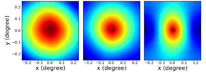
The beams are estimated independently for each array and season (Hasselfield et al., 2013, in preparation) from observations of Saturn following a procedure similar to the one described in Hincks et al. (2010). Radial beam profiles from the planet maps are transformed to Fourier space by fitting a set of basis functions whose analytic transform is known. The fit yields the beam transform as well as a covariance matrix following a procedure similar to that discussed in D11. The transform is subsequently corrected for the mapper transfer function, the solid angle of Saturn, and the difference in Saturn’s spectrum compared to the CMB blackbody spectrum. Because any location in the ACT CMB maps contains data from many different nights, the effective beam in the maps is broadened relative to the planet-based beam due to pointing variation from night to night. This pointing variation ($\simeq 6\arcsec$) is modelled as having a two-dimensional Gaussian distribution, and the standard deviation is measured by comparing the shape of the beam obtained from stacked radio sources to the planet-based beam transform. The error in the beam due to the pointing correction is included in the final beam covariance matrix. The covariant error in the beam is obtained after fixing the normalization of the beams at $\ell=700~{}(1500)$ for the 148 GHz (218 GHz) array. The calibration error is thus separated from the covariant error due to beam shape uncertainty, which is 0 by construction at $\ell=700~{}(1500)$.

2.5. Comparison with WMAP and South Pole Telescope Maps

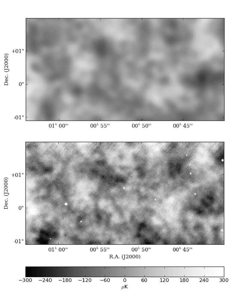
Fig. 5 shows a comparison between the WMAP 7-year 94 GHz map (Jarosik et al., 2011), and the 148 GHz and 218 GHz ACT maps on the same region of the sky. On the one hand, it exemplifies how our map-making pipeline faithfully reproduces all the large-scale CMB features seen in the WMAP map, and on the other hand it portrays the significantly higher resolution afforded by ACT over WMAP. This figure is a visual representation of the fact that the transfer function in our maps are unity down to small angular scales ($\ell\simeq 300$) or large spatial scales ($0\hbox{$.\!\!^{\circ}$}6$) – this proves highly beneficial for calibrating our maps against the WMAP maps, as discussed later.

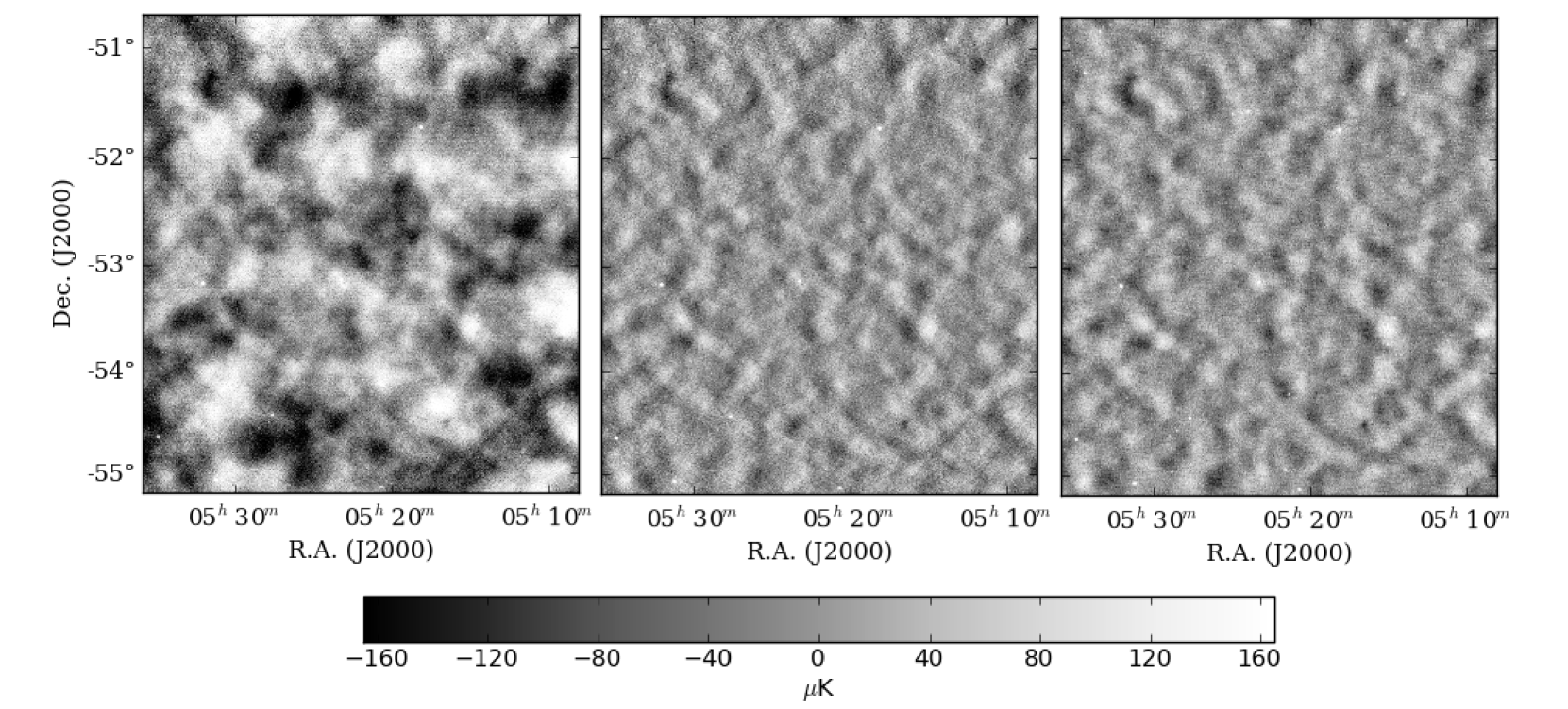
We also compare ACT maps with publicly released maps from the South Pole Telescope (Schaffer et al., 2011) in the region of overlap in the southern strip. Fig. 6 shows a side by side comparison between the ACT map co-added across all seasons and the SPT map on the same region of the sky. In the middle panel, the ACT map has been filtered with the same filter used for the SPT map. The similarity between the two maps is clear by eye, and speaks to the high quality of both measurements. A comparison of this figure with Fig. 13 of Dünner et al. (2012) (which used only 2008 observations) shows the improvement in the noise properties of the ACT map from the combination of multi-season observations.

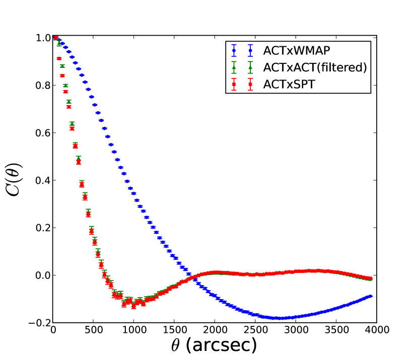
Using the techniques described in Hajian et al. (2011), we also studied the two-dimensional real-space correlation function (cf. equation 3 of Hajian et al. 2011) between the ACT and the SPT maps. Both the 2D cross correlation and the binned 1D version are shown in Fig. 7. The cross-correlation is anisotropic as the SPT map is filtered in the $\ell_{x}$ direction to suppress modes below $\ell_{x}\lesssim 1200$, but the overall agreement between the two experiments is excellent.

Figure 7.— Top: Two-dimensional cross-correlation function in real space between WMAP and ACT 148 GHz map (left panel), between ACT 148 GHz and ACT 218 GHz maps (middle panel), and between the ACT 148 GHz  and the SPT 150 GHz map from Schaffer et al. (2011). Note that the ACT-SPT cross-correlation is anisotropic as the SPT map is filtered in the $\ell_{x}$ direction to suppress modes below $\ell_{x}\lesssim 1200$. Bottom: One-dimensional binned version of real space correlation functions. The blue dots represent the 1D ACT 148 GHz $\times$ WMAP correlation, while the green triangles represent the 1D auto-correlation of ACT 148 GHz  maps after the SPT filter has been applied to them. Finally, the red squares denote the 1D cross-correlation of the ACT 148 GHz map with the SPT map.

3. Calibration

The final map calibration is performed in two stages: first, the 148 GHz map from the lowest-noise season is calibrated against the WMAP sky map, and then the 148 GHz maps from the remaining seasons and 218 GHz maps from all seasons are calibrated against the WMAP-calibrated 148 GHz map.

3.1. WMAP Calibration

ACT map-making and observing strategies result in maps with unbiased large-angle modes that can be compared to WMAP maps of the same region. The maps are cross-linked, i.e. every point in the survey has been observed during both its rising and setting. The cross-linked data are fed to a map-making pipeline described in Dünner et al. (2012) that allows the reconstruction of all modes in the map without biasing the large-angle modes. The transfer function of the maps is unity to better than 1% at angular scales corresponding to $\ell>300$ (Dünner et al., 2012). We calibrate the 148 GHz ACT maps directly to WMAP 7-year 94 GHz maps (Jarosik et al., 2011) of the identical regions using the cross-correlation method described in Hajian et al. (2011). By matching the ACT-WMAP cross-spectrum to the ACT power spectrum and the WMAP 7-year power spectrum (Larson et al., 2011) in the range $300<\ell<1100$, we calibrate the 148 GHz ACT spectrum to 2% fractional temperature anisotropy uncertainty (Hajian et al., 2011). Calibration to WMAP is done on the deepest seasons for both ACT-E and ACT-S strips, which correspond to season 4e (2010 observing season) and season 2sf (2008 observing season) data respectively. These calibrated maps are used as references to calibrate other seasons as described below.

3.2. Relative Season Calibration

Once the deepest 148 GHz  season has been calibrated with respect to WMAP, we cross-correlate that map with a 148 GHz map from another season, take the ratio of the cross-season cross-power spectrum to the in-season cross-power spectrum, and fit for a calibration factor. For example, on the equator, the 148 GHz  season 4e map is calibrated with respect to WMAP. We then compute the ratio $C_{\ell}^{4e\times 4e}/C_{\ell}^{3e\times 4e}$ to estimate the calibration for the season 3e 148 GHz map. This internal method lets us use a much wider range of angular scales (we use an $\ell$ range of width 2000 starting at $\ell=500$ for 148 GHz  and $\ell=1000$ for 218 GHz) than possible with WMAP. Using this method, we achieve the following relative calibration uncertainties (expressed as $\sigma_{X-Y}$ for season X calibrated against season $Y$) : $\sigma_{3e-4e}\simeq 0.7\%$, $\sigma_{3s-2s}\simeq 3\%$, and $\sigma_{4s-2s}=3\%$ for 148 GHz, and $\sigma_{3e-4e}\simeq 2\%$, $\sigma_{3s-2s}\simeq 9\%$, and $\sigma_{4s-2s}=4\%$ for 218 GHz maps. Note that for the ACT-S season 3s maps the calibration uncertainties are higher, as is expected from the fact that this season is largely noise dominated on most scales (see Fig. 4). The internal spectrum from this season gets highly downweighted in our likelihood. To tie together the 148 GHz and 218 GHz internal calibrations, we finally calibrate the best season 218 GHz map with respect to its 148 GHz counterpart, achieving $\sigma_{2s(218)-2s(148)}\simeq 1.3\%$, and $\sigma_{4e(218)-4e(148)}\simeq 1.7\%$. This gives the overall calibration of the reference 218 GHz map as $2.4\%$ for ACT-S and $2.6\%$ for ACT-E.

4. Temperature Power Spectrum Analysis

The power spectrum analysis methods used here are essentially the same as in D11, the major modifications being due to the smaller extent of the ACT-E maps in the declination direction compared to ACT-S, and the multi-season nature of the spectra.

4.1. Preprocessing of maps

We follow D11 and apply a high-pass filter to the maps to suppress the large angular scale modes ($\ell<500$) which are not as well constrained as others, and can bleed power into the smaller-scale modes. Next, we prewhiten the maps through real space operations as in D11.

4.2. Data Window

Each patch is then multiplied with a data window before the power spectrum is computed. The window is a product of three components: a point source mask, an apodization window, and the $n_{\mathrm{obs}}$ map giving the number of observations in each pixel. The point source mask is further described in Section 5.2. To simplify the application, we create a single $n_{\mathrm{obs}}$ map per patch by adding the individual $n_{\mathrm{obs}}$ maps from all the splits involved (four splits for the single frequency spectrum, and the 8 splits for the cross-frequency or cross-season spectrum), and apply this as a weight function. This essentially downweights the poorly observed regions of the patch. An additional step is applied to the ACT-E patches. Since the ACT-E strip is only 3 degrees wide, the absolute Fourier space resolution in the declination direction is $\Delta\ell_{y}=120$. This leads to instability in the mode-mode coupling calculations due to poor sampling of power in the Fourier space. To remedy this, we extend the patches in the declination direction by adding a 0.7-degree-wide-strip of zero valued pixels on either side, such that the final declination width of the zero-padded patch is 4.4 degrees. To minimize ringing from the edges of the patch, we also apply an apodization window which is generated by taking a top-hat function that is unity in the center and zero over 10 pixels at the edges of the original patch, and convolving it with a Gaussian of full width at half maximum of 2$\farcm$5 for ACT-S and 14$\farcm$0 for ACT-E. Another addition to the pipeline for the ACT-E patches is the application of a Galactic dust mask (see Section 5.1). Monte Carlo simulations demonstrate that we retrieve an unbiased estimate of the spectrum with these additions to our well-tested pipeline.

4.3. Binning of the power spectrum

It is important to note that the narrow inherent width of the ACT-E strip, as well as the smaller dimensions of the mulitseason ACT-S patches prompted us to adopt wider bins for the bandpowers than were used in D11. Most notably, over the acoustic peaks ($\ell<2000$) the bins used have a width $\Delta\ell=100$ as opposed to $\Delta\ell=50$ of D11. This choice is motivated by the fact that with the finer binning, adjacent bins remain significantly correlated for the ACT-E spectrum. In addition, evaluating the covariance using full end-to-end Monte Carlo simulations is prohibitively expensive given the iterative nature of our map-making process. Conversely, more tractable approximations might not be good enough to provide the precision deserved by the high quality of the data. With the larger bins we have verified that the bin-to-bin correlations never exceed 10% and are much smaller than 10% for most bin pairs, allowing us to treat the bandpowers as statistically independent (cf. Section 7.1) .

Figure 8.— Top: The IRIS 100 µm map on the ACT-E strip (arbitrary color scale). Bottom: The equatorial dust mask based on the IRIS map flux cut as described in the text. The small box near right ascension of ${00}^{\mathrm{h}}{14}^{\mathrm{m}}$ shows the “seagull”-like structure that is additionally masked out even though some pixels fall below the flux cut.

4.4. Cross-Season Cross-Spectrum Estimation

To obtain unbiased estimates of the cross spectrum we follow the same steps as enumerated in Section 3.6 of D11, which involve deconvolving a mode-coupling matrix that accounts for the effects of beam profile, prewhitening, filtering, pixelization, and windowing. For same-season cross spectra, the combinatorics are exactly the same as in D11: we compute 6 cross spectra per patch for the single-frequency spectrum (the 4 “splits” in time giving rise to the 6 cross spectra), and 12 for the cross-frequency spectrum (avoiding crossing the same splits that contain data from the same nights). For cross-season spectra we combine all 16 cross-season cross-spectra, as each split from one season has independent noise from the splits in the other season. For each frequency and season pair, the cross-spectra from the patches are combined with inverse variance weighting. This results in a set of three bandpowers $\{C_{b}^{3e\times 3e},C_{b}^{3e\times 4e},C_{b}^{4e\times 4e}\}$ for ACT-E  and a set of six bandpowers $\{C_{b}^{2s\times 2s},C_{b}^{2s\times 3s},C_{b}^{2s\times 4s},C_{b}^{3s\times 3s},C_{b}^{3s\times 4s},C_{b}^{4s\times 4s}\}$ for ACT-S, for each of the two same-frequency pairs $148\times 148$ and $218\times 218$. For the cross-frequency spectra $148\times 218$, where $C_{b}^{3e(148)\times 4e(218)}$ is distinct from $C_{b}^{4e(148)\times 3e(218)}$, we get a set of four bandpowers for ACT-E and nine bandpowers for ACT-S. These add up to a total of 10 cross-power spectra for ACT-E and 21 cross-power spectra for ACT-S that enter the likelihood separately with their individual bandpower covariance matrices. Additionally, there are six cross-power spectra coming from the full-footprint 2008 ACT-S map (2sf), which is added, with proper attention to the overlap between the s2f and s2 patches.

4.5. Bandpower Covariance

For each cross-power spectrum above, we evaluate a bandpower covariance matrix:

$$\Theta^{(\alpha A\times\beta B);(\gamma C\times\tau D)}_{bb} = \left\langle\left(\hat{C}_{b}^{\alpha A\times\beta B}-\left\langle\hat{C}_{b}^{\alpha A\times\beta B}\right\rangle\right)\right.$$ (1)

$$\times\left.\left(\hat{C}_{b}^{\gamma C\times\tau D}-\left\langle\hat{C}_{b}^{\gamma C\times\tau D}\right\rangle\right)\right\rangle$$

where we used Greek indices $\alpha$, $\beta$, etc. to denote the seasons 3e, 2s, etc. and the uppercase Roman numerals $A$, $B$, etc. to denote frequencies. The analytic expression of the general term of this covariance matrix $\Theta^{(\alpha A\times\beta B);(\gamma C\times\tau D)}_{bb}$ is discussed in the Appendix. The total covariance matrix is a sum of two terms: a sample covariance part accounting for the fact that different seasons of observation at different frequencies are observing the same CMB modes and that some of our cross spectra have common noise, and another part coming from the covariance of uncertainties in the determination of the beam profile. The covariance matrix is computed analytically and checked against Monte Carlo simulations described in Section 6. This total covariance matrix is used in defining the likelihood function (Dunkley et al., 2013; Sievers et al., 2013) when determining cosmological parameters.

Along with the covariance matrices, we also generate bandpower window functions which convert a theoretical power spectrum into a band power: $C_{b}^{\rm{th}}=\sum_{\ell}~{}B_{b\ell}C_{\ell}^{th}$. Due to different geometry and noise properties of the ACT-E and ACT-S patches, two separate window functions $B_{b\ell;ACT-s}$ and $B_{b\ell;ACT-e}$ are evaluated for the south and the equator.

4.6. Combining Multi-Season Spectra

For the purpose of parameter estimation, we keep the ACT-E and ACT-S spectra and covariances for each season separate in the likelihood (Dunkley et al., 2013). For display purposes and for visual comparison with other datasets we combine the spectra from different seasons (separately for equator and south) using inverse variance weighting:

$$\tilde{C}^{A\times B}_{b}=\frac{\sum_{\alpha,\beta}(\Theta^{-1})^{(\alpha A\times\beta B);(\alpha A\times\beta B)}_{bb}C_{b}^{(\alpha A\times\beta B)}}{\sum_{\alpha,\beta}(\Theta^{-1})^{(\alpha A\times\beta B);(\alpha A\times\beta B)}_{bb}}.$$ (2)

As discussed in Dunkley et al. (2013) the amplitudes of the Galactic cirrus contributions to the ACT-E and ACT-S maps are different. Therefore, before combining the ACT-E and ACT-S spectra obtained above, we subtract the best-fit cirrus component (see 5.1 for more details) from the ACT-E and ACT-S spectra, and then combine them using inverse variance weighting. The multiple levels of cross-correlation used in computing the power spectrum help ensure that potential peculiarities in the observation that are located in time or space do not propagate to the final power spectrum.

5. Foregrounds

In the 148 GHz and 218 GHz bands the main foregrounds are emission from point sources and diffuse Galactic dust, which we treat with the application of masks as described below. In the companion papers Dunkley et al. (2013) and Sievers et al. (2013) we also consider and constrain contributions from thermal and kinetic Sunyaev Zaldovich effects, clustered and Poisson-like infrared point sources, radio sources, and a residual Galactic cirrus component.

5.1. Galactic Dust

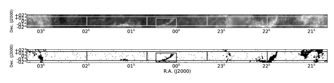
We detect a significant contribution from Galactic cirrus in our ACT-E maps, especially at 218 GHz. We employ a two-step approach for dealing with Galactic cirrus in the ACT-E maps using 100 $\mathrm{\SIUnitSymbolMicro}$m dust maps from IRIS (Miville-Deschênes & Lagache, 2005) as the reference. The first step is motived by the observation that most of the dust contamination in the equatorial power spectrum comes from the regions corresponding to bright clustered structures in the dust map. Therefore, we generate a dust mask by identifying and setting to zero all pixels above a flux density of 5.44 MJy/sr as well as pixels that fall inside significantly clustered structures such as the “seagull”-like structure near right ascension of ${00}^{\mathrm{h}}{14}^{\mathrm{m}}$ shown inside the box in Fig. 8. This dust mask is multiplied by the point source mask described below to generate the final mask that is applied to the data.

The second step of the dust treatment is generating a model of the residual dust contamination after the application of this mask, and then to inform the parameter estimation pipeline with reasonable priors on this model (the residual model amplitude is fitted and marginalized over when constraining cosmological parameters, as described in Dunkley et al. 2013). The model is constructed as follows. Following Hajian et al. (2012) we perform a multicomponent fit to the auto-power spectrum of the IRIS map after application of the dust mask described above. The components include a power law term for the residual Galactic cirrus, a Poisson shot noise term, a term representing the clustered component of infrared emission, and a white noise term to describe the instrument. The Galactic cirrus component is modeled as $C_{\ell}^{\rm{cirrus}}=A_{\rm{cirrus}}~{}\ell^{-2.7}$, where the value of the power law index appears to be a good fit to Herschel observations of cirrus (Miville-Deschênes et al., 2010; Bracco et al., 2011), as well as the cross correlation between ACT and BLAST (Hajian et al., 2012), and that between ACT and IRIS maps. This fitting procedure provides us with an estimate of the amplitude $A_{\rm{cirrus}}$ separately for the ACT-E and the ACT-S map footprints. Next, we cross-correlate the ACT maps with the IRIS template to evaluate the dust coefficient $A_{d}=C_{\ell}^{\rm{ACT}\times\rm{IRIS}}/C_{\ell}^{\rm{IRIS}\times\rm{IRIS}}$ for each frequency and each sky region. Finally, the cirrus contribution to the ACT power spectrum can be expressed as $C_{\ell}^{\rm{gal}}=A_{\rm{cirrus}}A_{d}^{2}~{}\ell^{-2.7}$ or expressed in terms of a rescaled amplitude at $\ell_{0}=3000$: ${\cal B}_{\ell}\equiv\ell^{2}C_{\ell}/(2\pi)=a_{\rm{g}}\left(\ell/{\ell_{0}}\right)^{-0.7}$, where we have defined $a_{\rm{g}}\equiv A_{\rm{cirrus}}~{}A_{d}^{2}~{}\ell_{0}^{-0.7}/(2\pi)$.

Table 2 Coefficients for Galactic cirrus model

Region	$A_{\rm{cirrus}}$	Frequency	$A_{d}$	$a_{g}$
	MJy2	GHz	µK/MJy
ACT-S	9.95	148	8.65	0.4
		218	30.0	5.2
ACT-E	17.9	148	8.65	0.8
		218	30.0	9.4

The various model parameters obtained from the fitting method above are displayed in Table 2. There is roughly twice as much dust in the ACT-E region as in ACT-S, but at $\ell=3000$ and for 148 GHz it is less than 3% of the CMB signal. These values represent a frequency scaling consistent with the early release results from the Planck satellite (Planck Collaboration et al., 2011), and can be compactly written in flux units as ${\cal B}_{\ell}^{ij}=a_{g}(\ell/\ell_{0})^{-0.7}(\nu_{i}\nu_{j}/\nu_{0}^{2})^{\beta}$ $\mathrm{\SIUnitSymbolMicro}$K² with $\beta=1.8$, $\nu^{i}$ and $\nu^{j}$ the two frequencies being crossed, and $\nu_{0}=$148 GHz. Based on the scatter observed in these central values as well their variation depending on whether the clustering term is included in the fit, we adopt priors of $a_{gs}=0.4\pm 0.2$ and $a_{ge}=0.8\pm 0.2$ for ACT-S and ACT-E respectively. The fitted models and priors are illustrated in Fig. 9.

Figure 9.— Galactic cirrus contributions to the power spectrum modeled as a power law as described in the text, for each frequency and region of the sky. The curves correspond to the best fit amplitudes obtained by cross-correlating ACT maps with cirrus component of the IRIS maps, and the band around them represent the uncertainty adopted as a prior in the ACT likelihood as discussed in Dunkley et al. (2013).

5.2. Point Sources

Point sources are the main astrophysical foreground for the 148 and 218 GHz bands. At these frequencies, point sources are typically either radio-loud AGN or dusty star-forming galaxies. Most of the bright sources are AGN, while most of the dusty star-forming galaxies lie below the detection threshold of our survey. Point sources must be identified and masked before the power spectrum is computed so as not to add power to the cosmological signal. We have identified sources using a matched filter algorithm (e.g., Tegmark & de Oliveira-Costa, 1998). We mask data within a 5 ′ radius around all sources detected down to 15 mJy in either band. The residual power contributed to the power spectrum from unmasked sources below our detection threshold is expected to be $2.9\pm 0.4~{}\mathrm{\SIUnitSymbolMicro}$K² at $l=3000$ (Gralla et al., in preparation). For details about the point source detection algorithm we used, and catalogs for the south 2008 148 GHz data, see Marriage et al. (2011). Catalogs for the remaining data set will be published in subsequent papers.

6. Simulations

We ran a set of Monte Carlo (MC) simulations in order to validate the analytic prescription for the uncertainties on the cross-season cross-frequency power spectra, and to investigate bandpower covariance and possible biases in the pipeline. As our map-making procedure is iterative, it is prohibitively expensive to run a large set of end-to-end simulations that would capture all aspects of the map-making pipeline, and the noise characteristics and correlations in the actual data set. Instead, following D11, we generate signal maps as Gaussian random realizations from a power spectrum, and add to each of them a realization of a Poisson point source population, and a simulated noise map generated from the observed noise-per-pixel in the data maps. The details of the implementation are essentially the same as in Section 4 of D11 with special care taken so that signal realizations are properly correlated across different seasons and footprints. For each season and each frequency, we generate 960 signal+noise maps (four splits for each frequency), and for each realization we compute the power spectra in exactly the same way as we do for the data maps. From the large set of cross-power spectra obtained in this way we estimate the season-season covariance as well as the correlation between band powers. We find that in all cases, correlation between adjacent bins are insignificant at the 10% level.

We evaluate the uncertainties in the band powers using an analytic prescription described in Appendix A. We verify the accuracy of these expressions by comparing the predicted error bars with the scatter of MC realizations. For isotropic white noise realizations with uniform weights, our expressions for multi-season multi-frequency error bars are good to better than a percent.

7. Temperature Power Spectrum Results

Table 3Single frequency combined bandpowers provided for plotting purposes only.
${\cal B}_{b}=\ell_{b}(\ell_{b}+1)C_{b}/2\pi$ ( µ K ²)

		148 GHz		148 GHz $\times$ 218 GHz		218 GHz
$\ell$ range	central $\ell_{b}$	${\cal B}_{b}$	$\sigma({\cal B}_{b})$	${\cal B}_{b}$	$\sigma({\cal B}_{b})$	${\cal B}_{b}$	$\sigma({\cal B}_{b})$
540 - 640	590	2267.4	114.3	-	-	-	-
640 - 740	690	1760.2	79.4	-	-	-	-
740 - 840	790	2411.2	97.0	-	-	-	-
840 - 940	890	1962.4	75.5	-	-	-	-
940 - 1040	990	1152.2	42.8	-	-	-	-
1040 - 1140	1090	1208.7	43.2	-	-	-	-
1140 - 1240	1190	1057.7	36.0	-	-	-	-
1240 - 1340	1290	743.1	25.7	-	-	-	-
1340 - 1440	1390	833.3	27.3	-	-	-	-
1440 - 1540	1490	683.0	22.0	-	-	-	-
1540 - 1640	1590	484.7	16.4	494.0	15.7	551.2	30.0
1640 - 1740	1690	403.1	13.3	400.6	12.6	458.5	26.9
1740 - 1840	1790	377.7	12.3	369.7	11.5	408.3	23.9
1840 - 1940	1890	266.8	9.3	272.7	9.3	327.0	20.3
1940 - 2040	1990	236.5	8.7	261.3	8.8	320.2	20.5
2040 - 2140	2090	229.2	8.1	226.6	7.7	274.7	17.9
2140 - 2340	2240	150.2	4.3	168.6	4.6	238.7	12.3
2340 - 2540	2440	109.2	3.5	128.1	3.8	199.8	10.7
2540 - 2740	2640	75.0	3.0	97.5	3.3	181.6	9.8
2740 - 2940	2840	63.7	2.9	86.0	3.2	181.9	9.6
2940 - 3340	3140	43.9	1.9	69.4	2.1	167.3	6.4
3340 - 3740	3540	35.7	2.0	65.2	2.1	183.6	6.5
3740 - 4140	3940	36.1	2.4	68.3	2.3	211.4	7.3
4140 - 4540	4340	34.4	2.8	75.5	2.7	245.7	8.3
4540 - 4940	4740	37.3	3.4	93.8	3.3	286.8	9.8
4940 - 5840	5390	50.5	3.2	109.8	3.0	355.8	9.5
5840 - 6740	6290	59.5	5.2	149.6	4.6	478.0	14.6
6740 - 7640	7190	81.6	8.7	177.9	6.6	564.4	19.9
7640 - 8540	8090	131.4	14.6	240.1	10.7	753.1	29.6
8540 - 9440	8990	133.0	25.5	265.3	16.6	878.7	44.3

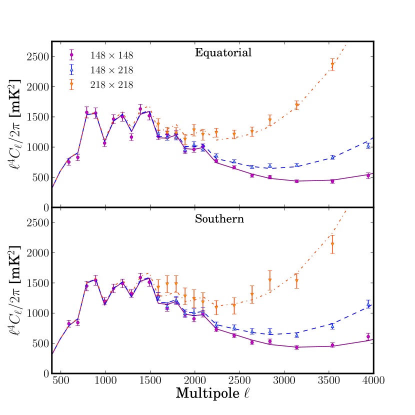
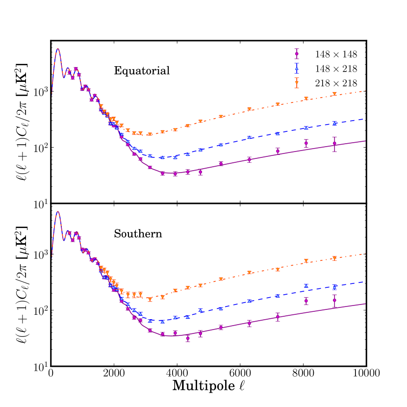
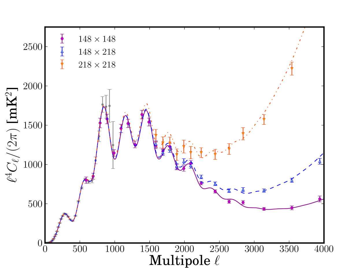
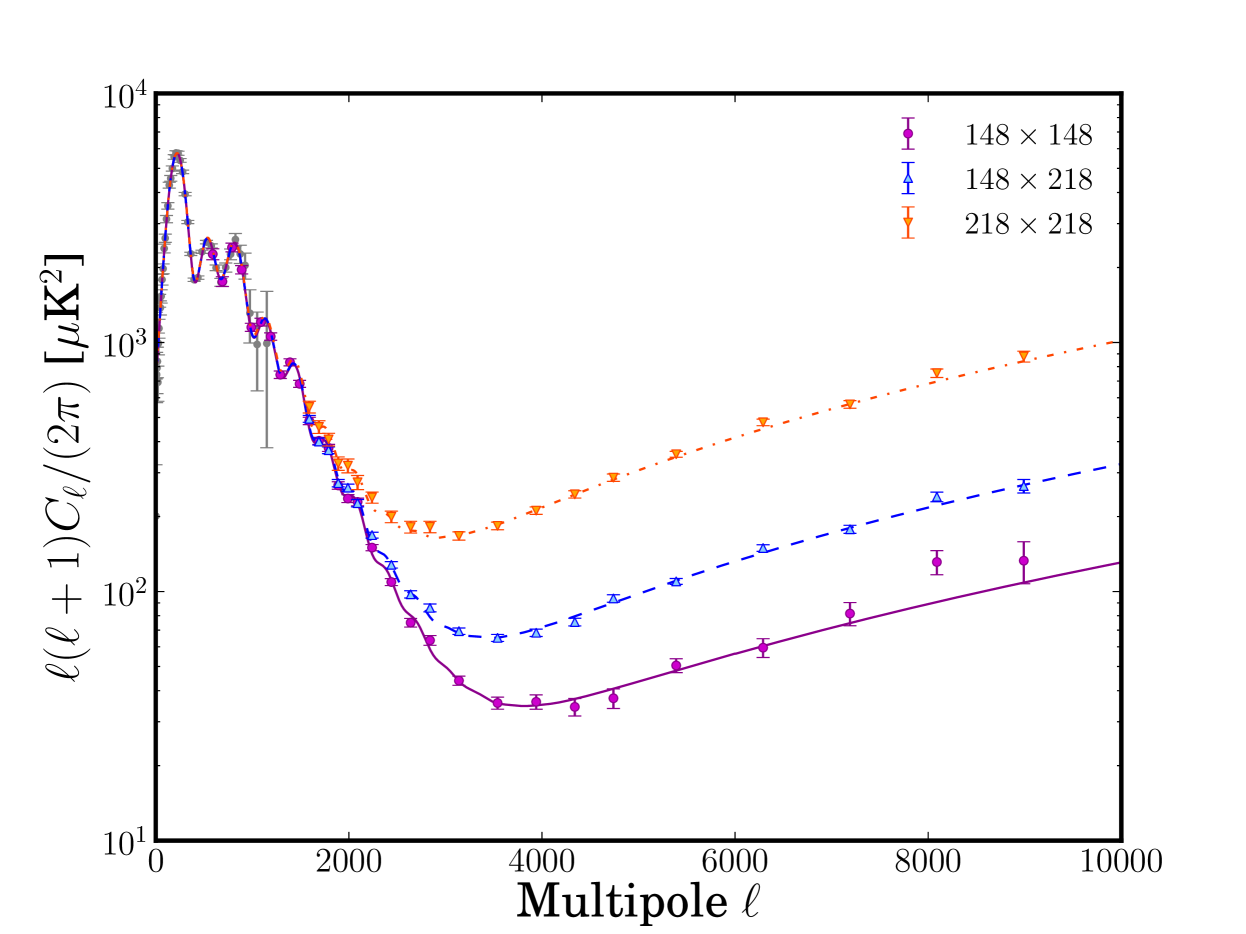
Power spectra are computed following the procedure outlined in Section 4 separately for each region (south and equator) and for each season pair. The entire set of spectra along with their covariance is passed on to the likelihood code that forms the basis of parameter constraints. Although combined spectra are not used in the actual analysis, in this section we discuss various combinations of power spectra for purposes of comparison and systematic tests. Note that ACT-S and ACT-E spectra cannot be trivially combined as residual Galactic cirrus contribution to the two regions are different. Therefore, we subtract the best fit residual cirrus model (as discussed in Dunkley et al. 2013) from the estimated power spectra before combining ACT-E and ACT-S spectra. To simplify the presentation, all figures in this section portray dust-subtracted spectra. Another complication arises due to the different geometries and masking pattern of the ACT-E and ACT-S maps, which cause the theoretical bandpowers for these regions to be in principle different, although the actual differences are small. Also, due to subtle variations of the beam profile from one season to another, the beam uncertainties in individual season spectra are slightly different. All these subtleties prompted the separate treatment of power spectra in the likelihood. In this section, we neglect these subtleties and combine spectra, with inverse variance weight, across season pairs and regions of the sky. We warn the reader hat such combinations are for visualization purposes only. Fig. 10 shows the ACT-E and ACT-S spectra combined across the different observing seasons, along with their corresponding theoretical band powers. The power spectrum combined across all seasons and across the ACT-E and ACT-S strips is displayed in Fig. 11. The corresponding band power values and uncertainties are tabulated in Table 3. These plots portray how our pipeline is able to produce an estimate of the power spectrum over the entire multipole range of $500-10000$. Over the multipole range of $\ell\simeq 500-2500$ these spectra clearly show the Silk damping tail of the CMB power spectrum, while on smaller angular scales ($\ell\sim 2500-10000$) a clear excess from the frequency-dependent Sunyaev Zel’dovich effects and extragalactic foregrounds (radio and infrared point sources) is clearly visible (these contributions are further discussed in Dunkley et al. 2013).

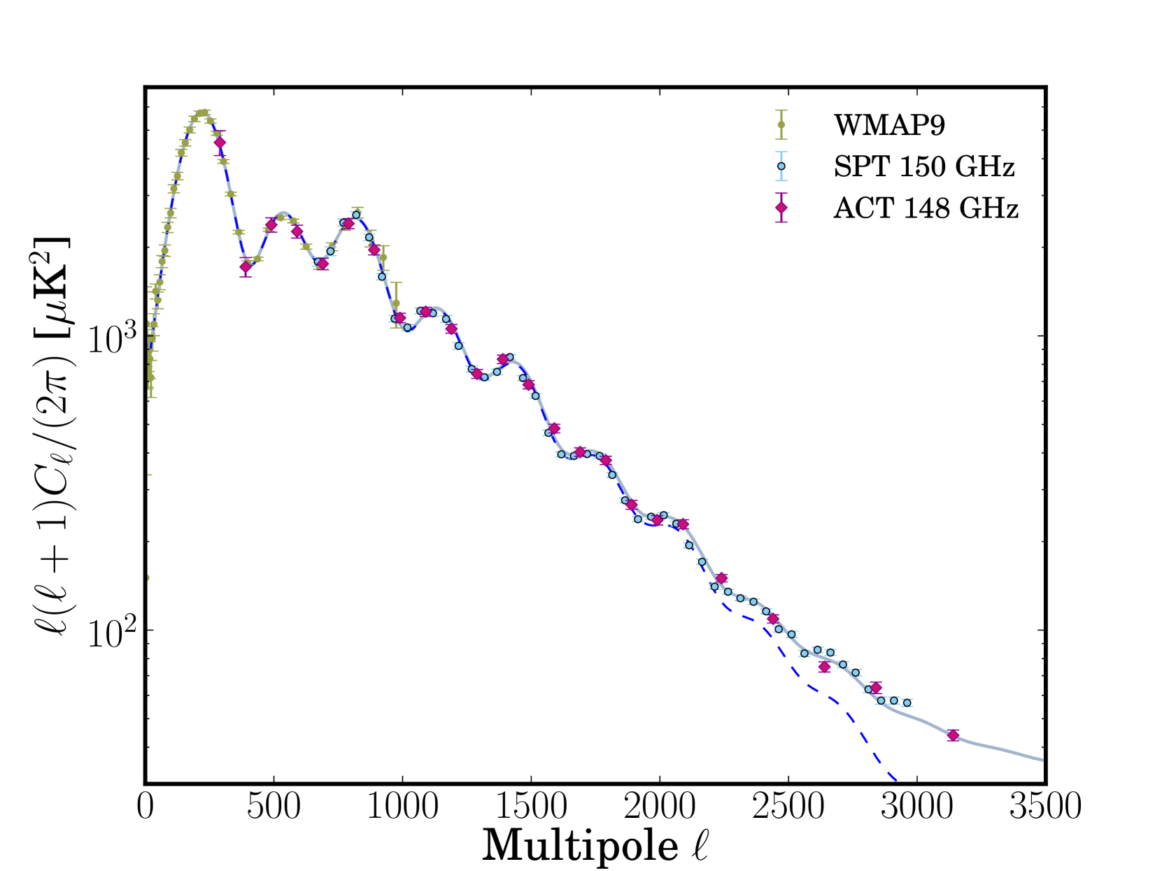
Finally, we display, in Fig. 12, the state of the art in CMB temperature power spectrum measurements down to the damping tail where we plot the WMAP 7-year spectrum, the inverse variance combined ACT-E+ACT-S spectrum, and the recent SPT power spectrum (Story et al., 2012).

7.1. Power spectrum with alternative binning

As discussed in Section 4.3, the choice of large bins for our main power spectrum result was motivated by the need for keeping the bandpowers minimally correlated. It is of interest, however, to ask how the spectrum would have looked with smaller bins of width $\Delta\ell=50$ over the damping tail, as was done in D11. Such a result is shown in Fig. 13. Note that the first through the eighth peak of the CMB can be clearly seen with this binning. We do not pursue this binning any further for the aforementioned reasons.

7.2. Derived CMB-only power spectrum

The ACT-E  and ACT-S spectra shown in Fig. 10 include the primary CMB signal as well as power from foregrounds and SZ. We show the estimated primary CMB spectrum from ACT in Fig. 14, derived in Dunkley et al. (2013). There, the multi-frequency spectra are used to estimate the CMB in bandpowers for ACT-E and ACT-S, simultaneously with the SZ and foregrounds components. The CMB spectra for ACT-E and ACT-S are then coadded for display. No assumptions are made about the cosmological model, only that the CMB is blackbody. Using the multi-frequency data to separate components, the CMB power can be recovered out to multipoles of $\ell\sim 3500$.

Figure 10.— Combined multi-season power spectra for the ACT-E Strip (upper panels) and the ACT-S Strip (lower panels). For the ACT-E and ACT-S data points, the corresponding best fit residual cirrus model (as discussed in Dunkley et al. 2013) has been subtracted. The left hand panel shows a linear scale zoomed-in version of the spectrum with an $\ell^{4}$ scaling to emphasize the higher order acoustic features. The lines show the binned version of the best fit model for each frequency pair including CMB secondaries and foregrounds from our companion paper Dunkley et al. (2013). The right panel shows the entire range of the computed spectrum on a log-linear scale with the conventional $\ell(\ell+1)$ scaling. The lines show the unbinned version of the best fit model from Dunkley et al. (2013).

Figure 11.— Multifrequency power spectra combined across all seasons and the ACT-E and ACT-S regions. Before combining the ACT-E and ACT-S data points, the corresponding best fit residual cirrus model (as discussed in Dunkley et al. 2013) has been subtracted. The upper panel shows the $\ell=500-4000$ portion of the power spectrum on a linear scale with an $\ell^{4}$ scaling to emphasize the higher order acoustic peaks. The lower panel shows the entire range of the computed spectra with the $\ell(\ell+1)$ scaling. The lines in either case show the best fit models for each frequency pair including CMB secondaries and foregrounds from our companion paper Dunkley et al. (2013). The grey data points represent the power spectrum from the WMAP seven-year data release (Larson et al., 2011).

Figure 12.— State of the art of CMB temperature power spectrum measurements from the WMAP 9-year data release (Bennett et al., 2012; Hinshaw et al., 2012), the South Pole Telescope (Story et al., 2012) and ACT (this work). The solid line shows the best fit model to the ACT 148 GHz data combined with WMAP 7-year data (Larson et al., 2011). The dashed line shows the CMB-only component of the same best fit model. Although we compute the power spectrum down to $\ell=200$, we do not use data below $\ell=540$ in the analysis.

Figure 13.— Combined ACT-E + ACT-S 148 GHz  power spectrum computed with alternate binning shown alongside the WMAP 9-year data (Bennett et al., 2012; Hinshaw et al., 2012). Note that with these smaller bins, the contours of the first seven acoustic peaks of the CMB power spectrum can be clearly seen. The bandpowers are significantly correlated at this bin size, and a precise estimate of the bin to bin correlation is computationally prohibitively costly. The solid line shows the best fit model to the ACT 148 GHz data combined with WMAP 7-year data (Larson et al., 2011).

Figure 14.— The CMB power spectrum estimated from ACT, shown with the spectrum from the WMAP 9-year data (Bennett et al., 2012; Hinshaw et al., 2012). The errors include uncertainty due to foreground and SZ emission, as well as the relative calibration of the 148 and 218 GHz channels, and beam uncertainty. The full covariance matrix is derived in Dunkley et al. (2013). The solid line shows the CMB-only component of the best fit model for the ACT data combined with the WMAP 7-year data.

7.3. Systematic Tests

In order to check for systematics in the map-making and power spectrum estimation pipelines, we perform various tests on the data. These are constructed such that the sky signal cancels between the various splits of the data, and only systematic effects remain. We test that the power spectrum obtained is the same in each season, in all time splits, from different parts of the array, with and without data near the telescope turnaround points, from different directions in Fourier space, and for different regions of the sky. The statistics from a subset of these tests are summarized in Tables 4, 5, 6, and 7. Given that the spectra are computed individually and then included in the likelihood with the full covariance of the different frequencies and seasons, we compute the null tests on each subset of data, both for ACT-E and ACT-S, and for different seasons.

7.3.1 Cross season nulls

Table 4Null test $\chi^{2}$ values for the season consistency tests performed on the ACT data. The probability to exceed (PTE) the $\chi^{2}$ is shown in parentheses.

Frequency	Region	Seasons	Seasons	Seasons	dof
		2008-2009	2009-2010	2008-2010
148 GHz	South	32.2 (0.36)	30.7 (0.43)	35.0 (0.24)	30
	Equator	-	39.7 (0.11)	-	30
220 GHz	South	27.7 (0.11)	15.9 (0.72)	21.5 (0.37)	20
	Equator	-	24.2 (0.23)	-	20

First, we test the year-to-year consistency of power spectra. In order to account for differences in the ACT beam from one observing season to the next, we convolve the map from one season with the beam profile of the other season being differenced, so that each map effectively has the same beam transfer function. Then we difference the corresponding splits from seasons $s_{1}$ and $s_{2}$:

$$\Delta T^{i}(\hat{\mathbf{n}})\equiv[T^{i}_{s_{1}}(\hat{\mathbf{n}})-T^{i}_{s_{2}}(\hat{\mathbf{n}})],$$ (3)

where i = 1,2,3,4 represent the split index. The pixel weight map $W$ corresponding to these difference splits is computed as:

$$W^{-1}=W^{-1}_{s_{1}}+W^{-1}_{s_{2}},$$ (4)

where $W_{s_{1}}$ is the total $N_{\rm{obs}}$ map for season $s_{1}$ etc. As with the other null tests, the azimuthal weighting is computed using the weights from the full data spectrum run. Figure 15 shows these test for the ACT data, while the individual $\chi^{2}$ values for the tests are summarized in Table 4. We find all spectra computed in this way to be consistent with null.

$\begin{array}[]{@{\hspace{-0.25in}}l}\includegraphics[width=234.15189pt]{cross_newAzv2.eps}\\ \end{array}$

Figure 15.— Cross season null test for the ACT data. The top row illustrate the 148 GHz cross season null tests for ACT-E (top left) and ACT-S (top right), while the bottom row show the 218 GHz cross season nulls.The $\chi^{2}$ values for the fit are presented in Table 4 and Figure 17.

7.3.2 Split Nulls

Table 5$\chi^{2}$ (PTE) values for the TOD split null tests performed on the ACT data.

Frequency	Region	Season		TOD		dof
			(1-2)x(3-4)	(1-3)x(2-4)	(1-4)x(2-3)
148 GHz	South	2008	19.7 (0.92)	37.7 (0.16)	37.1 (0.17)	30
		2009	30.3 (0.45)	31.8 (0.38)	22.6 (0.83)	30
		2010	35.7 (0.22)	28.6 (0.54)	21.5 (0.87)	30
	Equator	2009	33.9 (0.29)	26.5 (0.65)	40.9 (0.09)	30
		2010	34.6 (0.26)	35.6 (0.22)	24.0 (0.77)	30
220 GHz	South	2008	33.1 (0.03)	28.2 (0.10)	15.3 (0.76)	20
		2009	14.4 (0.81)	11.3 (0.94)	14.8 (0.79)	20
		2010	8.8 (0.99)	16.0 (0.72)	21.0 (0.40)	20
	Equator	2009	24.9 (0.21)	19.3 (0.50)	13.3 (0.87)	20
		2010	11.8 (0.92)	16.3 (0.70)	14.0 (0.83)	20

$\begin{array}[]{@{\hspace{-0.25in}}l}\includegraphics[width=234.15189pt]{splits_newAzv2.eps}\end{array}$

Figure 16.— TOD null test for the 148 GHz Southern strip, from 2008 (top panel) to 2010 (bottom panel). For each year, three TOD nulls are created from the combinations described in Eq. 7.3.2. The $\chi^{2}$ values for the null test are summarised in Table 5.

As discussed in Section 4, the data in each season are separated into four splits in such a way that the detector noise is independent from one split to another. Therefore, the difference between any two splits should be consistent with noise and the signal should subtract away. We test this by generating difference maps from each pair, and computing the two-way cross spectra from independent pairs of difference maps, e.g.:

$$T^{12}(\hat{\mathbf{n}})\equiv[T^{1}(\hat{\mathbf{n}})-T^{2}(\hat{\mathbf{n}})]/2$$

$$T^{34}(\hat{\mathbf{n}})\equiv[T^{3}(\hat{\mathbf{n}})-T^{4}(\hat{\mathbf{n}})]/2.$$ (5)

The difference maps are expected to contain noise but no residual signal. We estimate the cross-spectrum of the difference maps, $\hat{C}_{b}=\left<T^{12}T^{34}\right>,$ and the other two permutations of the differences ($\left<T^{13}T^{24}\right>$ and $\left<T^{14}T^{23}\right>$). These difference maps are downweighted by the same weight maps used to construct the full power spectrum. Similarly, the azimuthal weights are borrowed from the full data spectrum run. The three difference spectra are shown in Figure 16 for the 148 GHz ACT-S data set. The statistics corresponding to this test are shown in Table 5. The spectra are found to be consistent with a null signal, as expected.

7.3.3 In/Out nulls

In order to test for systematic detector asymmetries, we make a map using data from detectors from the inner region of the array, and another map from detectors along the edges, and compute the differences between the two maps:

$$T^{12}_{io}(\hat{\mathbf{n}}) \equiv [T^{1}_{o}(\hat{\mathbf{n}})-T^{2}_{i}(\hat{\mathbf{n}})]/2$$

$$T^{34}_{io}(\hat{\mathbf{n}}) \equiv [T^{3}_{o}(\hat{\mathbf{n}})-T^{4}_{i}(\hat{\mathbf{n}})]/2$$ (6)

where the $i$ and $o$ label the inner and outer parts of the detector array respectively. The full set of $\chi^{2}$ values are summarized in Table 6. In general we see no trend for differences as a function of detector position; the null tests are consistent with no signal.

Table 6Null test $\chi^{2}$ (PTE) values for the inner vs outer detectors.

Frequency	Region	Season		In/Out		dof
			(1o-2i)x(3o-4i)	(1o-3i)x(2o-4i)	(1o-4i)x(2o-3i)
148 GHz	South	2008	26.2 (0.66)	28.2 (0.56)	26.2 (0.67)	30
		2009	37.7 (0.16)	17.3 (0.97)	27.3 (0.61)	30
		2010	34.7 (0.26)	27.3 (0.61)	25.6 (0.70)	30
	Equator	2009	32.0 (0.36)	24.8 (0.74)	26.2 (0.66)	30
		2010	32.2 (0.36)	36.3 (0.20)	38.6 (0.13)	30
218 GHz	South	2008	25.3 (0.19)	23.9 (0.24)	21.0 (0.40)	20
		2009	13.7 (0.85)	12.3 (0.91)	25.8 (0.17)	20
		2010	13.8 (0.84)	15.0 (0.78)	26.3 (0.16)	20
	Equator	2009	23.4 (0.27)	22.6 (0.31)	27.9 (0.11)	20
		2010	9.9 (0.97)	25.3 (0.19)	9.2 (0.98)	20

$\begin{array}[]{@{\hspace{-0.05in}}l}\includegraphics[width=216.81pt]{chi2histv4.eps}\end{array}$

Figure 17.— The reduced $\chi^{2}$ values for all null tests. The blue histogram is computed for the $\chi^{2}$ values from the 218 GHz null tests, while the purple histogram shows the same null tests for the 148 GHz maps. The black dashed and dot-dashed lines show the theoretical distributions for 20 (AR2) and 30 (AR1) degrees of freedom respectively, normalized to match the frequency of the histograms. The $\chi^{2}$ values presented here are given in Tables 4, 5, 6 and 7.

7.3.4 Turnarounds

Another null test, based on cutting out data around telescope turnaround probes the consistency of data taken with the telescope accelerating as it reverses direction at the ends of the scan (turnarounds). In the maps used for the power spectrum estimation, the data taken during the turnaround is included. We test for any artifacts generated by the acceleration at turnaround by taking the difference of maps with and without turnaround data. Maps are made cutting data near the turnarounds, amounting to removing $\approx 10\%$ of the total data. This loss of data affects the two sky regions differently. In the southern patches, the loss of data is uniform and leads to a slight increase in striping in the maps, whereas in the equatorial patches, removing the turnarounds removes data at the upper and lower edges of the maps. Hence, for these tests we compute the differences using an equatorial region which is slightly narrower in the declination direction ($2\hbox{$.\!\!^{\circ}$}7$ as opposed to $3\deg$ wide). Two difference maps are made by pairing one split of the standard map with a different split of the new maps (we avoid differencing the same splits as they have very similar noise structure), and a two-way cross-power spectrum is produced. Any artifact due to the turnaround would be left in these difference maps and might produce excess power. We compute the turnaround cuts as a function of season, frequency range and area on the sky. The reduced $\chi^{2}$ values are summarized in Table 7. Again, we find that the difference maps have spectra consistent with no signal.

7.3.5 $\chi^{2}$ Distribution

While the null tests are performed for different subsets of the data, we combine the statistics from the null tests together to test for consistency globally. We restrict the range of the 218 GHz spectrum to be $\ell>1500$, hence the 218 GHz spectrum contains 20 degrees of freedom, while the 148 GHz spectrum containts 30 degrees of freedom. We show the distribution of $\chi^{2}$ values and the theoretical $\chi^{2}$ distribution for the two cases in Figure 17. This shows that the null tests are broadly consistent with being drawn from a $\chi^{2}$ distribution for the number of degrees of freedom.

7.3.6 Isotropy

Figure 18.— The two dimensional 148 GHz cross-power spectrum co-added across the ACT-E patches and seasons. For $\ell<2500$ smoothing by a small kernel has been applied. The acoustic features in the power spectrum are clearly visible. At $\ell>2500$, where the instrument noise dominates, we display the raw spectrum. The black lines represent the CMB-only theory and have been plotted to guide the eye.

Table 7Null test $\chi^{2}$ values for turnarounds

Frequency	Region	Season		Turnarounds		dof
			(1t-2nt)x(3t-4nt)	(1t-3nt)x(2t-4nt)	(1t-4nt)x(2t-3nt)
148 GHz	South	2008	21.9 (0.85)	24.8 (0.74)	34.6 (0.26)	30
		2009	28.3 (0.56)	35.3 (0.23)	26.7 (0.64)	30
		2010	30.5 (0.44)	30.4 (0.44)	35.0 (0.24)	30
	Equator	2009	27.4 (0.60)	29.3 (0.50)	34.0 (0.28)	30
		2010	35.1 (0.24)	43.9 (0.05)	21.9 (0.86)	30
218 GHz	South	2008	25.9 (0.17)	25.3 (0.19)	20.6 (0.42)	20
		2009	15.8 (0.73)	13.0 (0.88)	14.3 (0.82)	20
		2010	11.2 (0.94)	11.6 (0.93)	21.1 (0.4)	20
	Equator	2009	31.3 (0.06)	19.4 (0.5)	16.6 (0.68)	20
		2010	14.1 (0.82)	24.3 (023)	16.7 (0.67)	20

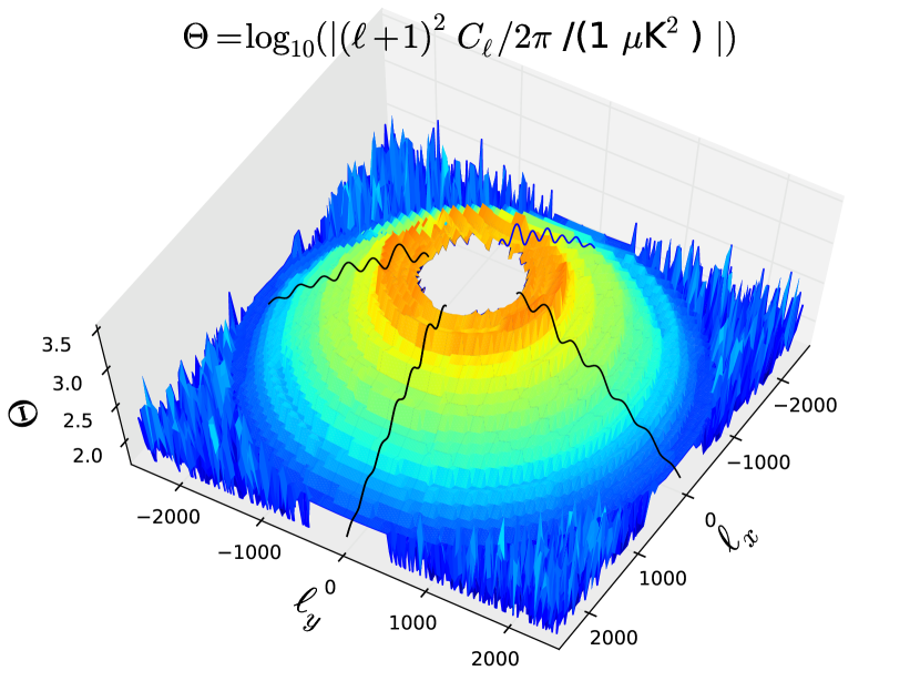
We test the isotropy of the power spectrum by estimating the power as a function of phase $\theta=\arctan(\ell_{y}/\ell_{x})$. We compute the inverse-noise-weighted two-dimensional spectrum co-added across patches and seasons for the ACT-E region. We show the mean two-dimensional cross-power pseudo spectrum in Figure 18. The spectrum is symmetric for $\ell$ to $-\ell$, as it is for any real valued map. To quantify any anisotropy, the power averaged over all multipoles in the range $200<\ell<10000$ is computed in wedges of $\theta=20^{\circ},$ and compared to the mean of the entire annulus. No significant deviation from isotropy is detected using this method. We find that this result holds for ACT-S and 218 GHz maps.

7.4. Consistency of ACT-E, ACT-S, and SPT spectra

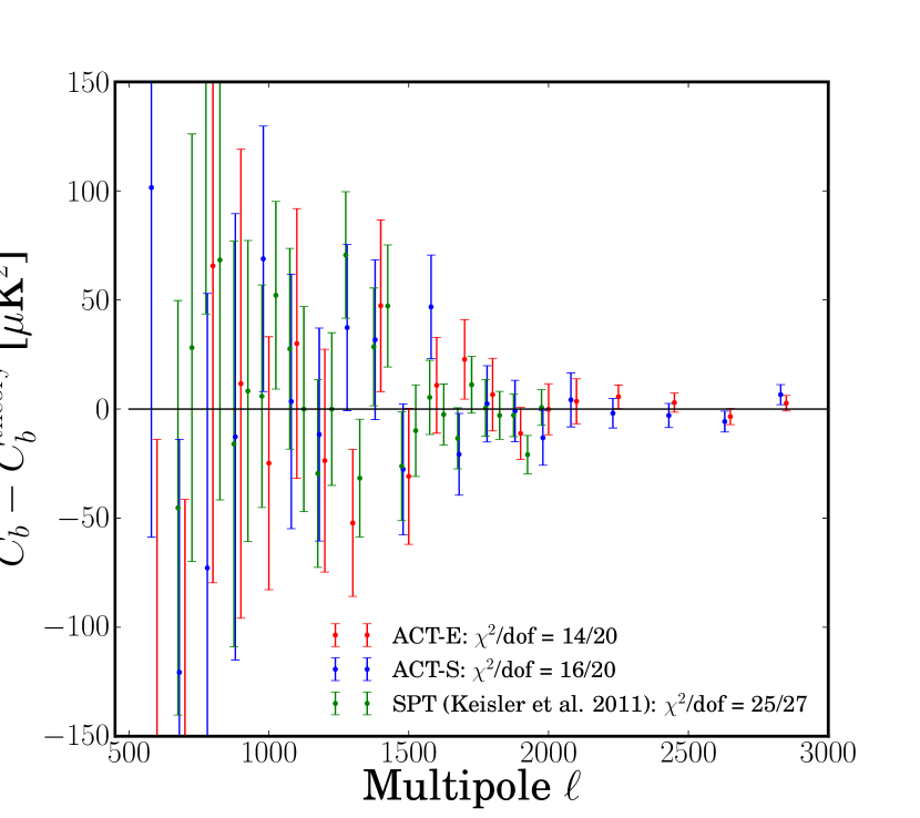
As mentioned above, due to the difference in geometry of the equatorial vs. southern patches, the band power binning functions for ACT-E and ACT-S are slightly different leading small differences in the binned version of the best fit ACT $+$ WMAP7 model (Sievers et al., 2013). Therefore to test the consistency between ACT-E and ACT-S  spectra we check for the nullity of the residuals from their corresponding binned best fit model. We also consider the consistency of the SPT band powers from Keisler et al. (2011). Care must be taken while computing the residual for the SPT spectrum as the point source masking threshold corresponding to that spectrum was different from that of ACT. To correct for this, we adjust the Poisson point source component of our best fit model to match the masking level used in Keisler et al. (2011). The results are shown in Fig. 19, clearly indicating that the three spectra are consistent with null, and therefore with each other.

Figure 19.— The residual power spectra obtained after subtracting the best fit ACT + WMAP model from the ACT-E, ACT-S, and SPT power spectrum (Keisler et al., 2011). For the SPT residual the Poisson point source component of the best fit model is adjusted to reflect the difference in point source masking levels between ACT and SPT. The residuals are all null showing the consistency of these spectra.

The suite of consistency tests performed here show that our reported spectrum passes a wide range of checks for systematic errors in time, detector-space, map-space, and $\ell$-space.

8. Gravitational Lensing Analysis

Figure 20.— CMB convergence power spectrum reconstructed from the ACT-E strip temperature data. The enhanced effective depth of the coadded ACT-E map ($\simeq 18$ $\mu$k-arcmin) compared to its previous version ($\simeq 23$ $\mu$k-arcmin) used in Das et al. (2011a) led to an improved detection significance.

Large-scale structure gravitationally deflects the CMB radiation as it passes through the universe, thereby defining a lensing deflection field $\mathbf{d}$ that remaps the observed CMB temperature sky: $T(\hat{\mathbf{n}})=T_{\rm{unlensed}}(\hat{\mathbf{n}}+\mathbf{d})$. Lensing distorts the small-scale CMB anisotropies, thus modifying their statistical properties, with the lensing deflection locally breaking statistical isotropy and correlating formerly independent temperature Fourier modes (or more intuitively, correlating the CMB temperature with its gradient). The lensed small-scale CMB thus contains not only information about the universe at the last-scattering surface ($z\simeq 1100$), but also encodes information about the cosmic mass distribution at later times and lower redshifts. Using an estimator quadratic in temperature that measures the lensing-induced change in the statistics of the CMB fluctuations from the correlation of formerly independent Fourier modes, one can construct a noisy estimate of the CMB lensing convergence, $\kappa=-\frac{1}{2}\nabla\cdot\mathbf{d}$, which is a measure of the projected matter density out to high redshifts. The power spectrum of the CMB lensing convergence can be simply obtained from this estimated lensing convergence field, though biases arising from instrument and cosmic-variance-induced noise as well as from higher order corrections to the estimator must be subtracted. Equivalently the estimation of the lensing power spectrum can be regarded as a measurement of a lensing-induced non-Gaussianity in the CMB temperature four-point correlation function. Measurements of the lensing power spectrum can place strong constraints on the properties of dark energy and neutrinos, and also serve as a valuable test of the $\Lambda$CDM prediction for structure growth and geometry at redshifts $z\simeq 1-3$.

CMB lensing science has made great advances in recent years. Signatures of CMB lensing were first observed in correlations of the CMB with large-scale structure (Smith et al., 2007; Hirata et al., 2008). The lensing power spectrum was first detected at $4\sigma$ significance by the ACT collaboration (Das et al. 2011a). The first evidence for dark energy from the CMB alone was also obtained from this measurement by Sherwin et al. 2011. A more significant detection (at $6.3~{}\sigma$) of the lensing power spectrum and more precise cosmological constraints were reported by the SPT collaboration the following year (van Engelen et al., 2012).

In this work we present a measurement of the lensing power spectrum from the improved ACT maps on the ACT-E strip. Our new measurement of lensing essentially uses the same methodology as Das et al. (2011a), hereafter DS11. Lensing is measured using a quadratic estimator in temperature; the power spectrum of the CMB lensing convergence is thus a temperature four-point function with the filtering and normalization obtained as in DS11. The bias is calculated in three steps to make the calculation as robust and model-independent as possible. First, we simulate the bias that is present in the absence of any mode-correlations, removing existing correlations by randomizing the phases of each Fourier mode of the temperature field (DS11). This is mathematically equivalent to estimating the so-called $N(0)$ bias from the pseudo-$C_{\ell}$ power spectrum measured from this map. The use of measurements rather than simulations makes the bias calculation more robust. Next, we simulate additional small biases from finite-map effects, and anisotropic and inhomogeneous noise by performing lensing power spectrum estimation on unlensed simulated CMB maps with realistic noise characteristics. After accounting for these two sources of bias, the input lensing power spectrum is recovered fairly accurately in simulations, but there is a small difference between recovered and input power spectra due to higher order corrections. We adopt the small, simulated difference between the recovered and true power spectra as an additional bias and subtract it from the biased lensing power spectrum estimated from data.

Systematic contamination of the estimator by the SZ signal, IR and radio sources was estimated in DS11 using the simulations from Sehgal et al. (2010). The authors found that, with the ACT lensing pipeline as used in this work, the contamination is smaller than the signal by two orders of magnitude and can thus be neglected. This result appears well-motivated for two reasons, which also apply to our current analysis: first, in the analysis we only use the signal-dominated scales below $\ell=2300$, at which SZ, IR and radio power are subdominant; second, by using the data to estimate the bias, our estimator automatically subtracts the Gaussian part of the contamination, so that only a very small non-Gaussian residual remains. The previous ACT contamination estimates are not strictly applicable to the new lensing estimate, because the filters used here contain somewhat lower noise, and thus admit slightly more signal at higher $\ell$s; however, estimates by the SPT collaboration (van Engelen et al. 2012) with similar noise levels and filters also find negligible contamination. The contamination levels in our analysis are thus also expected to be negligible.

The measured CMB lensing power spectrum, detected at $4.6\sigma$, is shown in Fig. 20, along with a theory curve showing the convergence power spectrum for a fiducial $\Lambda$CDM model defined by the parameter set $(\Omega_{b},\Omega_{m},\Omega_{\Lambda},h,n_{s},\sigma_{8})$ = (0.044, 0.264, 0.736, 0.71, 0.96, 0.80). Constraining the conventional lensing parameter $A_{L}$ that rescales the fiducial convergence power spectrum ($C_{\ell}^{\kappa\kappa}\rightarrow A_{L}C_{\ell}^{\kappa\kappa}$) we obtain $A_{L}=1.06\pm 0.23$. The data are thus a good fit to the $\Lambda$CDM prediction for the amplitude of CMB lensing. As in DS11, we find the spectrum to have Gaussian errors, uncorrelated between bins. For some parameter runs, the lensing power spectrum information is added to the CMB power spectrum information (Sievers et al., 2013).

9. Conclusions

We have derived the power spectrum of microwave sky maps at 148 GHz and 218 GHz produced by the Atacama Cosmology Telescope experiment, such as those displayed in Fig. 5. The power spectra cover a range of angular scales spanning nearly a factor of 20, ranging from around 0.35 degrees ($\ell=590$) to a little over one arcminute ($\ell=8900$). The maps are high quality, and in principle extracting the power spectrum is a simple matter. A host of practical considerations, along with the precision supported by the data, make estimation of the power spectrum challenging. This paper summarizes algorithms and techniques for handling the particular shapes of our maps, point source contamination, the steepness of the power spectrum, significant features due to galactic dust emission, spatially varying noise levels, and calibration. In addition to the resulting power spectra, we also display numerous null tests on the data. These tests, along with results from simulated maps, make a strong case that any systematic errors in our power spectra are below the level of statistical error.

The ACT power spectra are consistent with those measured by the South Pole Telescope collaboration, as are the underlying maps in a region of overlapping sky coverage. Given how small the signals are and how many sources of error must be tamed to measure them, consistent results represent a substantial experimental achievement.

The temperature power spectrum measurements displayed in Figure 12 represent the culmination of a two-decade quest, since the first large-angle power measurements were made by the COBE satellite (Smoot et al., 1992). It was soon realized that for inflationary cosmological models, the substantial structure in the microwave background temperature angular power spectrum due to coherent acoustic oscillations in the early universe would allow precise constraints on the basic properties of the universe (Jungman et al., 1996). A series of innovative and increasingly sensitive experiments then gradually unveiled the power spectrum. With the definitive measurements down to quarter-degree scales by the WMAP satellite (Bennett et al., 2012) and the precise arcminute-scale measurements by ACT (this work) and SPT (Story et al., 2012) along with the results anticipated from the Planck satellite, this particular route to cosmological insight is approaching a highly refined state.

A new frontier in microwave background experiments will likely be detailed lensing maps from high-resolution polarization measurements (Niemack et al., 2010; Austermann et al., 2012), which have the prospect of constraining dark energy and modified gravity (e.g., Das & Linder 2012). The lensing power spectrum measurements presented here and by SPT (van Engelen et al., 2012) are the first steps along this new path.

Appendix A Analytic errorbars

Here we derive an analytic expression for the expected error bars on the cross-frequency mulitseason cross-power spectrum. We denote the frequencies with uppercase $A$, $B$, $C$, $D$, the seasons with $\alpha$, $\beta$, $\gamma$, $\tau$, and the sub-season data splits with $i$, $j$, $k$,$l$. Following D11, the covariance the of cross-power spectrum is defined as:

$$\Theta^{(\alpha A\times\beta B);(\gamma C\times\tau D)}_{bb}\equiv\langle(C_{b,\alpha\beta}^{(A\times B)}-\langle C_{b,\alpha\beta}^{(A\times B)}\rangle)(C_{b,\gamma\tau}^{(C\times D)}-\langle C_{b,\gamma\tau}^{(C\times D)}\rangle)\rangle,$$

which expands as

$$\Theta^{(\alpha A\times\beta B);(\gamma C\times\tau D)}_{bb}=\frac{1}{N}\frac{1}{\nu_{b}^{2}}\sum_{i,j,k,l}^{n_{d}}\sum_{\mbox{\boldmath$\ell$}\in b}\sum_{\mbox{\boldmath$\ell^{\prime}$}\in b}\left(\left[\left\langle T^{*iA}_{\mbox{\boldmath$\ell$},\alpha}T^{jB}_{\mbox{\boldmath$\ell$},\beta}T^{*kC}_{\mbox{\boldmath$\ell$}^{\prime},\gamma}T^{lD}_{\mbox{\boldmath$\ell$}^{\prime},\tau}\right\rangle\right]-\left\langle C_{b,\alpha\beta}^{(iA\times jB)}\right\rangle\left\langle C_{b,\gamma\tau}^{(kC\times lD)}\right\rangle\right)$$

$$\times(1-\delta_{ij}\delta_{\alpha\beta})(1-\delta_{kl}\delta_{\gamma\tau}).$$ (A2)

The Kronecker deltas remove the auto power spectra, and any same-split, same-season cross-frequency spectra. The general normalization is

$$N = \sum_{i,j,k,l}^{n_{d}}(1-\delta_{ij}\delta_{\alpha\beta})(1-\delta_{kl}\delta_{\gamma\tau})$$ (A3)

$$= n_{d}^{4}-n_{d}^{3}(\delta_{\alpha\beta}+\delta_{\gamma\tau})+n_{d}^{2}(\delta_{\alpha\beta}\delta_{\gamma\tau}).$$

Applying Wick’s Theorem, we have

$$\Theta^{(\alpha A\times\beta B);(\gamma C\times\tau D)}_{bb}=\frac{1}{\nu_{b}}\frac{1}{N}\sum_{i,j,k,l}^{n_{d}}\left[\left\langle C_{b,\alpha\gamma}^{iA\times kC}\right\rangle\left\langle C_{b,\beta\tau}^{jB\times lD}\right\rangle+\left\langle C_{b,\alpha\tau}^{iA\times lD}\right\rangle\left\langle C_{b,\beta\gamma}^{jB\times kC}\right\rangle\right]$$

$$\times(1-\delta_{ij}\delta_{\alpha\beta})(1-\delta_{kl}\delta_{\gamma\tau}),$$ (A4)

where

$$\left\langle C_{b,\beta\gamma}^{jB\times kC}\right\rangle=C_{b}+\delta_{jk}\delta_{BC}\delta_{\beta\gamma}N_{b}^{\beta\beta,BB}.$$ (A5)

Therefore, $\Theta^{(\alpha A\times\beta B);(\gamma C\times\tau D)}_{bb}$ expands to

$$\begin{split}&\Theta^{1;(\alpha A\times\beta B);(\gamma C\times\tau D)}_{bb}=2\frac{C_{b}^{2}}{\nu_{b}}+\frac{1}{N}\frac{C_{b}}{\nu_{b}}\sum_{i,j,k,l}^{n_{d}}\left[(\delta_{ik}\delta_{AC}\delta_{\alpha\gamma}N_{b}^{\alpha\alpha,AA}+\delta_{jl}\delta_{BD}\delta_{\beta\tau}N_{b}^{\beta\beta,BB})\right.\\ &\left.\quad{}+(\delta_{il}\delta_{AD}\delta_{\alpha\tau}N_{b}^{\alpha\alpha,AA}+\delta_{jk}\delta_{BC}\delta_{\beta\gamma}N_{b}^{\beta\beta,BB})\right]\times(1-\delta_{ij}\delta_{\alpha\beta})(1-\delta_{kl}\delta_{\gamma\tau})\\ &+\frac{1}{N}\frac{1}{\nu_{b}}\sum_{i,j,k,l}^{n_{d}}N_{b}^{\alpha\alpha,AA}N_{b}^{\beta\beta,BB}(\delta_{ik}\delta_{AC}\delta_{\alpha\gamma}\delta_{jl}\delta_{BD}\delta_{\beta\tau}+\delta_{il}\delta_{AD}\delta_{\alpha\tau}\delta_{jk}\delta_{BC}\delta_{\beta\gamma})\times(1-\delta_{ij}\delta_{\alpha\beta})(1-\delta_{kl}\delta_{\gamma\tau}),\end{split}$$ (A6)

which after some algebra reduces to

$$\begin{split}&\Theta^{(\alpha A\times\beta B);(\gamma C\times\tau D)}_{bb}=\frac{1}{\nu_{b}}\left(2C_{b}^{2}+\frac{C_{b}N_{b}^{\alpha\alpha,AA}}{n_{d}}(\delta_{AC}\delta_{\alpha\gamma}+\delta_{AD}\delta_{\alpha\tau})+\frac{C_{b}N_{b}^{\beta\beta,BB}}{n_{d}}(\delta_{BC}\delta_{\beta\gamma}+\delta_{BD}\delta_{\beta\tau})\right.\\ &\left.\quad{}+N_{b}^{\alpha\alpha,AA}N_{b}^{\beta\beta,BB}(\delta_{AD}\delta_{\alpha\tau}\delta_{BC}\delta_{\beta\gamma}+\delta_{AC}\delta_{\alpha\gamma}\delta_{BD}\delta_{\beta\tau})\frac{n_{d}^{2}-n_{d}(\delta_{\alpha\beta}+\delta_{\gamma\tau})+n_{d}(\delta_{\alpha\beta}\delta_{\gamma\tau})}{n_{d}^{4}-n_{d}^{3}(\delta_{\alpha\beta}+\delta_{\gamma\tau})+n_{d}^{2}(\delta_{\alpha\beta}\delta_{\gamma\tau})}\right)\end{split}$$ (A7)

Therefore, with $A\neq B\neq C$ and $\alpha\neq\beta$ we have,

$$\Theta^{(\alpha A\times\alpha A);(\alpha A\times\alpha A)}_{b} =\frac{1}{\nu_{b}}\left[2C_{b}^{2}+4\frac{C_{b}}{n_{d}}N_{b}^{\alpha\alpha,AA}+2\frac{(N_{b}^{\alpha\alpha,AA})^{2}}{n_{d}(n_{d}-1)}\right],$$ (A8)

$$\Theta^{(\alpha A\times\alpha B);(\alpha A\times\alpha B)}_{b} =\frac{1}{\nu_{b}}\left[2C_{b}^{2}+\frac{C_{b}}{n_{d}}(N_{b}^{\alpha\alpha,AA}+N_{b}^{\alpha\alpha,BB})+\frac{N_{b}^{\alpha\alpha,AA}N_{b}^{\alpha\alpha,BB}}{n_{d}(n_{d}-1)}\right],$$ (A9)

$$\Theta^{(\alpha A\times\alpha A);(\alpha A\times\alpha B)}_{b} =\frac{1}{\nu_{b}}\left[2C_{b}^{2}+2\frac{C_{b}N_{b}^{\alpha\alpha,AA}}{n_{d}}\right],$$ (A10)

$$\Theta^{(\alpha A\times\alpha A);(\alpha B\times\alpha B)}_{b} =\frac{1}{\nu_{b}}\left[2C_{b}^{2}\right],$$ (A11)

$$\Theta^{(\alpha A\times\alpha B);(\alpha A\times\alpha C)}_{b} =\frac{1}{\nu_{b}}\left[2C_{b}^{2}+\frac{C_{b}N_{b}^{\alpha\alpha,AA}}{n_{d}}\right],$$ (A12)

$$\Theta^{(\alpha A\times\beta A);(\alpha A\times\beta B)}_{b} =\frac{1}{\nu_{b}}\left[2C_{b}^{2}+\frac{C_{b}N_{b}^{\alpha\alpha,AA}}{n_{d}}\right],$$ (A13)

$$\Theta^{(\alpha A\times\beta A);(\alpha B\times\beta B)}_{b} =\frac{1}{\nu_{b}}\left[2C_{b}^{2}\right],$$ (A14)

$$\Theta^{(\alpha A\times\beta B);(\alpha A\times\beta C)}_{b} =\frac{1}{\nu_{b}}\left[2C_{b}^{2}+\frac{C_{b}N_{b}^{\alpha\alpha,AA}}{n_{d}}\right].$$ (A15)

Appendix B Including beam covariance in the estimate

We can also include the effect of an uncertainty on the beam when combining data between different season. We consider the covariance of the power spectrum for two season pairs: $i\times j$s and $k\times l$, with beam window functions $w^{i\times j}_{b}=B_{b}^{i}B_{b}^{j}$ and $w^{k\times l}_{b^{\prime}}=B_{b^{\prime}}^{k}B_{b^{\prime}}^{l}$, respectively. The measured windows function is given by $w^{obs}_{b}=w_{b}+\delta w_{b}$. This error propagates to the power spectrum covariance as

$$\langle\frac{w^{i\times j}_{b}C^{i\times j}_{b}}{w^{i\times j}_{b}+\delta w^{i\times j}_{b}}\frac{w^{k\times l}_{b^{\prime}}C^{k\times l}_{b^{\prime}}}{w^{k\times l}_{b^{\prime}}+\delta w^{k\times l}_{b^{\prime}}}\rangle\rightarrow\frac{C^{i\times j}_{b}}{w^{i\times j}_{b}}\frac{C^{k\times l}_{b^{\prime}}}{w^{k\times l}_{b^{\prime}}}\langle\delta w^{i\times j}_{b}\delta w^{k\times l}_{b^{\prime}}\rangle.$$ (B1)

The error on the window function is related to the error of the beam by

$$\delta w^{i\times j}_{b}=\delta B_{b}^{i}B_{b}^{j}+B_{b}^{i}\delta B_{b}^{j}.$$ (B2)

References

- Addison et al. (2012a) Addison, G. E., Dunkley, J., & Bond, J. R. 2012a, arXiv:1210.6697
- Addison et al. (2012b) Addison, G. E., et al. 2012b, ApJ, 752, 120
- Austermann et al. (2012) Austermann, J. E., et al. 2012, in Society of Photo-Optical Instrumentation Engineers (SPIE) Conference Series, Vol. 8452, Society of Photo-Optical Instrumentation Engineers (SPIE) Conference Series
- Bennett et al. (2012) Bennett, C. L., et al. 2012, arXiv:1212.5225
- Bracco et al. (2011) Bracco, A., et al. 2011, MNRAS, 412, 1151
- Brown et al. (2009) Brown, M. L., et al. 2009, ApJ, 705, 978
- Das & Linder (2012) Das, S., & Linder, E. V. 2012, Phys. Rev. D, 86, 063520
- Das et al. (2011a) Das, S., et al. 2011a, Physical Review Letters, 107, 021301
- Das et al. (2011b) —. 2011b, ApJ, 729, 62
- Dunkley et al. (2011) Dunkley, J., et al. 2011, ApJ, 739, 52
- Dunkley et al. (2013) —. 2013, arXiv:1301.0776
- Dünner et al. (2012) Dünner, R., et al. 2012, arXiv:1208.0050
- Fowler et al. (2010) Fowler, J. W., et al. 2010, ApJ, 722, 1148
- Friedman et al. (2009) Friedman, R. B., et al. 2009, ApJ, 700, L187
- Hajian et al. (2011) Hajian, A., et al. 2011, ApJ, 740, 86
- Hajian et al. (2012) —. 2012, ApJ, 744, 40
- Hall et al. (2010) Hall, N. R., et al. 2010, ApJ, 718, 632
- Hasselfield et al. (2013) Hasselfield, M., et al. 2013, in preparation
- Hincks et al. (2010) Hincks, A. D., et al. 2010, ApJS, 191, 423
- Hinshaw et al. (2012) Hinshaw, G., et al. 2012, arXiv:1212.5226
- Hirata et al. (2008) Hirata, C. M., Ho, S., Padmanabhan, N., Seljak, U., & Bahcall, N. A. 2008, Phys. Rev. D, 78, 043520
- Jarosik et al. (2011) Jarosik, N., et al. 2011, ApJS, 192, 14
- Jungman et al. (1996) Jungman, G., Kamionkowski, M., Kosowsky, A., & Spergel, D. N. 1996, Phys. Rev. D, 54, 1332
- Keisler et al. (2011) Keisler, R., et al. 2011, ApJ, 743, 28
- Larson et al. (2011) Larson, D., et al. 2011, ApJS, 192, 16
- Lueker et al. (2010) Lueker, M., et al. 2010, ApJ, 719, 1045
- Marriage et al. (2011) Marriage, T. A., et al. 2011, ApJ, 731, 100
- Miville-Deschênes & Lagache (2005) Miville-Deschênes, M.-A., & Lagache, G. 2005, ApJS, 157, 302
- Miville-Deschênes et al. (2010) Miville-Deschênes, M.-A., et al. 2010, A&A, 518, L104
- Niemack et al. (2010) Niemack, M. D., et al. 2010, in Presented at the Society of Photo-Optical Instrumentation Engineers (SPIE) Conference, Vol. 7741, SPIE Conference Series
- Planck Collaboration et al. (2011) Planck Collaboration et al. 2011, A&A, 536, A18
- Reichardt et al. (2009) Reichardt, C. L., et al. 2009, ApJ, 694, 1200
- Reichardt et al. (2012) —. 2012, ApJ, 755, 70
- Schaffer et al. (2011) Schaffer, K. K., et al. 2011, ApJ, 743, 90
- Sehgal et al. (2010) Sehgal, N., Bode, P., Das, S., Hernandez-Monteagudo, C., Huffenberger, K., Lin, Y., Ostriker, J. P., & Trac, H. 2010, ApJ, 709, 920
- Sherwin et al. (2011) Sherwin, B. D., et al. 2011, Physical Review Letters, 107, 021302
- Shirokoff et al. (2011) Shirokoff, E., et al. 2011, ApJ, 736, 61
- Sievers et al. (2009) Sievers, J. L., et al. 2009, arXiv:0901.4540
- Sievers et al. (2013) —. 2013, arXiv:1301.0824
- Smith et al. (2007) Smith, K. M., Zahn, O., & Doré, O. 2007, Phys. Rev. D, 76, 043510
- Smoot et al. (1992) Smoot, G. F., et al. 1992, ApJ, 396, L1
- Story et al. (2012) Story, K. T., et al. 2012, arXiv:1210.7231
- Sunyaev & Zeldovich (1972) Sunyaev, R. A., & Zeldovich, Y. B. 1972, Comments on Astrophysics and Space Physics, 4, 173
- Swetz et al. (2010) Swetz, D. S., et al. 2010, ArXiv e-prints
- Swetz et al. (2011) —. 2011, ApJS, 194, 41
- Tegmark & de Oliveira-Costa (1998) Tegmark, M., & de Oliveira-Costa, A. 1998, ApJ, 500, L83
- van Engelen et al. (2012) van Engelen, A., et al. 2012, ApJ, 756, 142
- Zahn et al. (2012) Zahn, O., et al. 2012, ApJ, 756, 65