Coupling between time series: a network view

Abstract

Recently, the visibility graph has been introduced as a novel view for analyzing time series, which maps it to a complex network. In this paper, we introduce a new algorithm of visibility, ”cross-visibility”, which reveals the conjugation of two coupled time series. The correspondence between the two time series is mapped to a network, ”the cross-visibility graph”, to demonstrate the correlation between them. We applied the algorithm to several correlated and uncorrelated time series, generated by the linear stationary ARFIMA process. The results demonstrate that the cross-visibility graph associated with correlated time series with power-law auto-correlation is scale-free. If the time series are uncorrelated, the degree distribution of their cross-visibility network deviates from power-law. For more clarifying the process, we applied the algorithm to real-world data from the financial trades of two companies, and observed significant small-scale coupling in their dynamics.

I Introduction

Coupled series, and series of long range correlations could not be thoroughly understood, unless a global view of them is represented Kantz et al. (1997). Complex networks Boccaletti et al. (2006); Newman (2003); Albert and Barabási (2002), on the other hand, have provided a global understanding of multi-component systems. Recently, the idea of complex networks has been implemented for single variable systems Jafari et al. (2011); Shirazi et al. (2009), and mapping between time series and networks is proposed. For example, nodes in such networks can be extracted by binning the time axis or the level axis Vahabi et al. (2011).

While some features of time series are not simply observed with standard approaches, they can be easily studied when converted to a network Nuñez et al. (2012). For example, financial trades, which their dynamics seem to be alike to a white noise, include memory Liu et al. (1997); Pasquini and Serva (1999); Mantegna and Stanley (1999) and represent high clustering when converted to complex networks. Moreover, investigating a map between time series and networks is a method of constructing several prototypes of complex networks Xie and Zhou (2011).

According to a recent work Lacasa et al. (2008), the visibility algorithm has been introduced as a fast computational algorithm of mapping a time series to a network. Several properties of the time series are served in the resulting network’s structure. For example, a periodic series results in a regular lattice, a fractal series results in a scale-free network and a random series is in correspondence with a random graph.

Visibility is the representation of the question that how much local information is attained from a global structure. Based on this approach, new global properties are introduced for time series. For example, along with scale-free properties, small-world characteristics Strogatz (2001) are demonstrated for the fractional Brownian motion time series Lacasa et al. (2008). Also, in order to distinguish randomness in time series, a modified visibility algorithm Luque et al. (2009) is proposed. Visibility algorithm is found to be an appropriate approach in different interdisciplinary areas. For example, the method is pertinent to social studies Fan et al. (2010). In addition, mathematical structures such as fractal and complex chaotic time series have been studied using the visibility algorithm Lacasa et al. (2008); Lacasa and Toral (2010).

In this work, we introduce a new visibility algorithm, based on the mutual information of two time series. We call this type of visibility the cross-visibility. According to this method, the visibility criterion is represented for two time series, i.e., a time series looks at its components through the obstacles of a second time series. This approach is especially appropriate for analyzing real-world data with power-law autocorrelation. The algorithm provides a framework to understand how complex time series lead each other, and determines the direction of information flow between them. In addition, coupling in different scales is demonstrated. Investigating the cross-visibility between well-known correlated and uncorrelated time series could be a criterion for characterizing the cross-visibility. For this purpose, we studied the fractional Gaussian noise (fGn) time series.

Previously, it has been demonstrated that the Hurst exponent for the fractional Brownian motion series is distinguished by the structure of the degree distribution in their visibility graph Lacasa et al. (2009). We extended this analysis for correlated fGn time series, and characterized the power-law exponent in the resulting cross-visibility networks’ degree distribution, according to their Hurst exponent. Also, in order to depict the implementation of the approach to real-world data, we used the data from recent financial trades for two companies. We depicted the information flow in several scales between pertinent data.

II The cross-visibility algorithm

According to the standard visibility algorithm  Lacasa et al. (2008), every component in the time series $\{y_{i}\}$, with $i=1\ldots N$, is mapped to a node of a graph. Node $i$ and node $j$ $(i<j)$ are connected, if they are visible to each other without any obstacles between them:

$$i<\forall k<j;\hskip 28.45274pty_{k}<y_{i}+\frac{y_{j}-y_{i}}{j-i}(k-i).$$ (1)

If node $i$ is visible to node $j$, node $j$ will also visible to node $i$. Therefore, the corresponding network is non-directional. Elements in the time series with amount high above the others have high degrees, and create the singular nodes of the network.

The cross-visibility algorithm maps two time series, $\{x_{i}\}$ and $\{y_{i}\}$, into two different networks, the cross-visibility networks. The algorithm consists of two major steps:

a. In order to make the time series comparable, they are normalized to reveal dimensionless variables. If the sequences are stationary, they are normalized to their mean and variances. Therefore, new sequences are generated as $\{\hat{x_{i}}\}=\{\frac{x_{i}-\bar{x}}{\sigma_{x}}\}$ and $\{\hat{y_{i}}\}=\{\frac{y_{i}-\bar{y}}{\sigma_{y}}\}$. $\bar{x}$ and $\bar{y}$ are the mean values of the series $\{x_{i}\}$ and $\{y_{i}\}$, respectively; $\sigma_{x}$ and $\sigma_{y}$ are the corresponding variances. If the series are non-stationary, they are normalized to their corresponding maximum value.

b. Every component in the time series $\{\hat{x}_{i}\}$ is mapped to a node of a graph. Node $i$ is connected to node $j$, if:

$$i<\forall k<j;\hskip 28.45274pt\hat{y}_{k}\leq\hat{y}_{i}+\frac{\hat{x}_{j}-\hat{x}_{i}}{j-i}(k-i)$$ (2)

or

$$i<\forall k<j;\hskip 28.45274pt\hat{y}_{k}\geq\hat{y}_{i}+\frac{\hat{x}_{j}-\hat{x}_{i}}{j-i}(k-i).$$ (3)

This rule could be interpreted as node $i$ looking at the components of $\{\hat{x}_{j}\}$ time series, through the obstacles of the shifted time series $\{\bar{y}_{j}\}=\{\hat{y}_{j}-\hat{y}_{i}+\hat{x}_{i}\}$. The structure of this network demonstrates how $\{x_{i}\}$ leads the time series $\{y_{i}\}$. Equation 2 refers to the visibility from the top view, and equation 3 demonstrates the visibility from the beneath view. We depict this graph as $G^{xy}$. However, another network, $G^{yx}$, could be generated by changing the role of $\{x_{i}\}$ and $\{y_{i}\}$.

The cross-visibility can bring a directional measure of mutual information between the time series. If the time series $\{y_{j}\}$ is permuted randomly to construct a time series ( $\{y^{p}_{j}\}$) uncorrelated to $\{x_{j}\}$, the structure of the cross-visibility network $G^{x,y^{p}}$ deviates from the original one. Each network could be evaluated through its degree distribution.

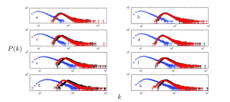
Figure 1: (Color on-line) Degree distribution for several cross-visibility networks corresponding to different Hurst exponents is depicted. (Blue) squares demonstrate the result for the coupled series, (red) stars are for the uncoupled series, and (black) triangles are for the permuted series. Coupling between several series with $H\in\{0.6,0.7,0.8,0.9,1\}$ is investigated. $0.6-0.7$ and $0.7-0.6$ are included in a and b, $0.6-0.8$ and $0.8-0.6$ are included in c and d, $0.6-0.9$ and $0.9-0.6$ are included in e and f, and $0.6-1$ and $1-0.6$ are included in g and h, respectively. Both axes are sketched in logarithmic scale.

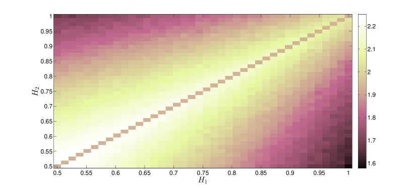
Figure 2: (Color on-line) The color plot demonstrates the exponent of the power-law degree distribution associated with the cross-visibility networks of coupled series with $H\in[0.5,1[$. The result is sketched for the cross-visibility networks $G^{H_{1},H_{2}}$, where $H_{1}$ and $H_{2}$ are the corresponding Hurst exponent for the first and the second time series, respectively.

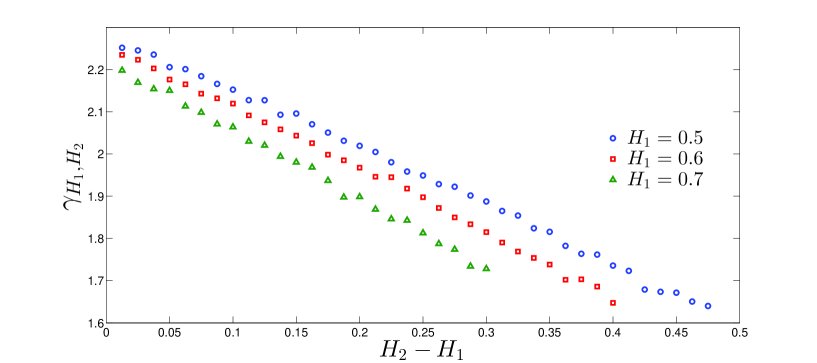
Figure 3: (Color on-line) Power-law exponent for the degree distribution of cross-visibility graphs associated with coupled time series is sketched as a function of the difference between the corresponding Hurst exponents. The result is depicted for different Hurst exponents, $H_{1}$, for the cross-visibility network $G^{H_{1},H_{2}}$. The power-law exponent decays linearly with $H_{2}-H_{1}$.

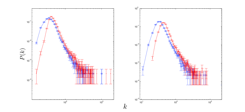
Figure 4: (Color on-line) The closing price of simultaneously recorded data for Microsoft and IBM is analyzed by the cross-visibility algorithm. Degree distribution associated with the original data is depicted by (blue) squares. (Red) dots depict the degree distribution for the cross-visibility network of permuted time series, $G^{x,y^{p}}$. The deviation is mostly concerned with the small scales, and also the pick of each distribution is shifted for uncoupled time series. Both axes are sketched in logarithmic scale.

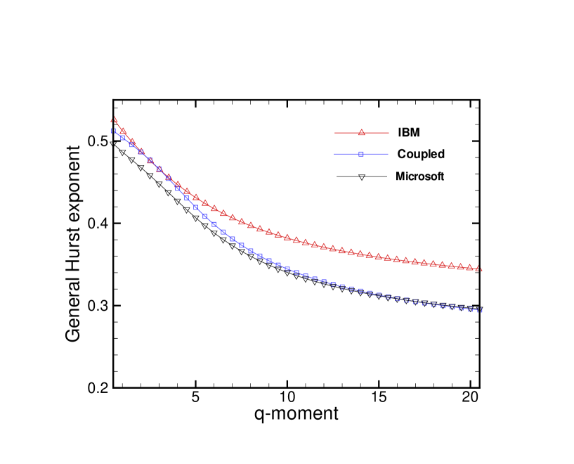
Figure 5: (Color on-line) General Hurst exponents IBM, Microsoft and their coupled estimated using multi-fractal detrended cross-correlation analysis.

II.1 Characterizing cross-visibility

In order to interpret the results from the cross-visibility algorithm, it is worthy to analyze the time series that are confirmed to be coupled or uncoupled. We investigated the time series generated by the linear stationary ARFIMA  Podobnik et al. (2007); Hosking (1981); Granger (1980) process. The analysis is a criteria for further investigations.

Through a stochastic recursive rule, the ARFIMA process generates a power law auto-correlated series $\{y_{k}\}$:

$$y_{i}=\sum_{j=1}^{\infty}a_{j}(\rho)y_{i-j}+\eta_{i},$$ (4)

where, $a_{j}(.)$ is a weight, defined due to an independent real variable $0<\rho<\frac{1}{2}$ as $a_{j}(\rho)=\frac{\Gamma(j-\rho)}{\Gamma(-\rho)\Gamma(1+j)}$. $\eta_{i}$, the error term, is a member of an i.i.d sequence, which consists of random normal distribution samples. The Hurst exponent, $H$, is related to $\rho$ as $H=0.5+\rho$  Hosking (1981). These time series depict power-law autocorrelation Horvatic et al. (2011), and If exactly same error sequence is used in generating the two time series, they show power-law cross correlation. In contrast, independent error terms reveal uncoupled time series.

We applied the cross-visibility algorithm to coupled time series, with different independent terms $\rho\in[0,0.5[$, which are in correspondence with Hurst exponents $H\in[0.5,1[$. FIG. 1 depicts the degree distribution associated with each network. A power-law degree distribution is demonstrated for the coupled series. The cross-visibility network for the uncoupled time series have completely different structure in contrast to the corresponding network of coupled series (stars and triangles in FIG. 1). Moreover, the average degree of the distributions is higher for the uncoupled series.

If the time series are correlated, the corresponding exponent of the power-law degree distributions, depicted as $\gamma_{xy}$ for $G^{xy}$, determine how the series are leading each other. $\gamma_{xy}$ for several series with Hurst exponents $H\in[0.5,1[$ is depicted as a color plot in FIG. 2. In order to determine the exponent of the degree distribution we used a maximum likelihood estimation (MLE)  Newman (2005). In FIG. 3 a linear dependency between $\gamma_{H_{1},H_{2}}$ and $H_{2}-H_{1}$ is depicted. This result demonstrates that the Hurst exponents could be distinguished by evaluating the power-law exponents. The result is sketched for several Hurst exponents $H_{1}$.

II.2 Application in empirical data

For real-world data, it is important to confirm if the time series are coupled and to what extent they follow each other. In order to determine the coupling between the two time series, $\{x_{i}\}$ and $\{y_{i}\}$, we put the associated degree distribution of their cross-visibility networks into contrast with the corresponding network of permuted time series.

We analyzed the cross-visibility between the closing price of two companies, Microsoft and IBM. The cross-visibility method is applied to the normalized logarithm of the prices. For each company, return prices are stationary and are normalized to their average and standard deviations. The degree distribution of the cross-visibility graphs associated with original series and permuted time series is depicted in Fig. 4. For the original series, the associated degree distribution is a power-law. However, if one of the series (the second series) is permuted, the associated degree distribution deviates from the original distribution. The most significant deviations are concerned with the small degrees. This however means that there is strong correlation in small fluctuations. Deviation in the tail of the distributions corresponding to high degrees is negligible. These time series do not follow each other in their high amplitude fluctuations. The value of the degree corresponding to the pick of the distribution is a characteristic of the lag time response between the two time series.

It is worthwhile to compare the results with the systematic obtaining of the cross-correlation analysis (DXA) Podobnik and Stanley (2008); Zhou (2008); Shadkhoo and Jafari (2009). Fig. 5 shows the results for DXA, and indicates how Microsoft leads coupling in higher moments and IBM in lower moments. One important difference is that DXA is a symmetric method to analyze the cross-correlation, but the cross-visibility introduces two networks of coupling between the two time series.

III Conclusions

- Understanding the coupling between two time series and how information transfers between them is a crucial concept in various areas of complex systems. For this purpose, in this paper we depicted this coupling as a network map.

- In general, as the coupling between two time series is asymmetric, there are two networks to present the coupling between them.

- Our results demonstrate that in average, the number of degrees corresponding to the coupled series is less than that of the uncoupled data. There is a shift in $P(k)$ to higher degrees in uncoupled time series, which could be a criteria to measure the value of coupling.

- Our findings show that, increasing the difference between the Hurst exponent of two fGn time series, the corresponding degree distribution decays with slower slope in higher degrees, which means higher coupling or higher correspondence between the two time series. This approach is appropriate for investigating coupling for different empirical data. In addition, through this approach the conjugation in different scales between time series could be studied. In the end, using this approach, the coupling between Microsoft and IBM has been viewed in two coupled networks.

References

- Kantz et al. (1997) H. Kantz, T. Schreiber, and R. Mackay, Nonlinear time series analysis, vol. 2000 (Cambridge university press Cambridge, 1997).
- Boccaletti et al. (2006) S. Boccaletti, V. Latora, Y. Moreno, M. Chavez, and D. Hwang, Physics reports 424, 175 (2006).
- Newman (2003) M. Newman, SIAM review 45, 167 (2003).
- Albert and Barabási (2002) R. Albert and A. Barabási, Reviews of modern physics 74, 47 (2002).
- Jafari et al. (2011) G. Jafari, A. Shirazi, A. Namaki, and R. Raei, Computing in Science & Engineering 13, 84 (2011).
- Shirazi et al. (2009) A. Shirazi, G. Jafari, J. Davoudi, J. Peinke, M. Tabar, and M. Sahimi, Journal of Statistical Mechanics: Theory and Experiment 2009, P07046 (2009).
- Vahabi et al. (2011) M. Vahabi, G. Jafari, and M. Movahed, Journal of Statistical Mechanics: Theory and Experiment 2011, P11021 (2011).
- Nuñez et al. (2012) A. Nuñez, L. Lacasa, J. Gomez, and B. Luque, New Frontiers in Graph Theory, InTech, Rijeka pp. 119–152 (2012).
- Liu et al. (1997) Y. Liu, P. Cizeau, M. Meyer, C. Peng, and H. Eugene Stanley, Physica A: Statistical Mechanics and its Applications 245, 437 (1997).
- Pasquini and Serva (1999) M. Pasquini and M. Serva, Economics Letters 65, 275 (1999).
- Mantegna and Stanley (1999) R. Mantegna and H. Stanley, Introduction to econophysics: correlations and complexity in finance (Cambridge University Press, 1999).
- Xie and Zhou (2011) W. Xie and W. Zhou, Physica A: Statistical Mechanics and its Applications 390, 3592 (2011).
- Lacasa et al. (2008) L. Lacasa, B. Luque, F. Ballesteros, J. Luque, and J. Nuño, Proceedings of the National Academy of Sciences 105, 4972 (2008).
- Strogatz (2001) S. Strogatz, Nature 410, 268 (2001).
- Luque et al. (2009) B. Luque, L. Lacasa, F. Ballesteros, and J. Luque, Physical Review E 80, 046103 (2009).
- Fan et al. (2010) C. Fan, J. Guo, and Y. Zha, arXiv preprint arXiv:1012.4088 (2010).
- Lacasa and Toral (2010) L. Lacasa and R. Toral, Physical Review E 82, 036120 (2010).
- Lacasa et al. (2009) L. Lacasa, B. Luque, J. Luque, and J. Nuno, EPL (Europhysics Letters) 86, 30001 (2009).
- Podobnik et al. (2007) B. Podobnik, D. Fu, H. Stanley, and P. Ivanov, The European Physical Journal B-Condensed Matter and Complex Systems 56, 47 (2007).
- Hosking (1981) J. Hosking, Biometrika 68, 165 (1981).
- Granger (1980) C. Granger, Journal of econometrics 14, 227 (1980).
- Horvatic et al. (2011) D. Horvatic, H. Stanley, and B. Podobnik, EPL (Europhysics Letters) 94, 18007 (2011).
- Newman (2005) M. Newman, Contemporary physics 46, 323 (2005).
- Podobnik and Stanley (2008) B. Podobnik and H. Stanley, Physical review letters 100, 84102 (2008).
- Zhou (2008) W. Zhou, Physical Review E 77, 066211 (2008).
- Shadkhoo and Jafari (2009) S. Shadkhoo and G. Jafari, The European Physical Journal B-Condensed Matter and Complex Systems 72, 679 (2009).