Scattering problems in the fractional quantum mechanics governed by the 2D space fractional Schrödinger equation

Jianping Dong
Department of Mathematics, College of Science, Nanjing University of Aeronautics and Astronautics, Nanjing 210016, China

The 2D space-fractional Schrödinger equation in the time-independent and time-dependent cases for the scattering problem in the fractional quantum mechanics is studied. We define and give the mathematical expression of the Green’s functions for the two cases. The asymptotic formulas of the Green’s functions are also given, and applied to get the approximate wave functions for the fractional quantum scattering problems.

1 Introduction

Nowadays, the fractional calculus [1, 2] becomes a useful tools for scientists. It has been successfully applied in anomalous transport, diffusion-reaction processes, super-slow relaxation, etc [4, 3]. Recently, the fractional calculus enters the world of quantum mechanics. In quantum physics, Feynman and Hibbs [7] reformulated the famous Schrödinger equation [8, 9] by use of the path integral approach considering the Gaussian probability distribution. The Lévy stochastic process is a natural generalization of the Gaussian process. The possibility of developing the path integral over the paths of the Lévy motion was discussed by Kac [10], who pointed out that the Lévy path integral generates the functional measure in the space of left (or right) continued functions having only discontinuities of the first kind. Recently, Laskin[11, 12, 13] generalized Feynman path integral to Lévy one, and developed a space-fractional Schrödinger equation containing the Riesz fractional derivative [1, 2]. Then, he constructed the fractional quantum mechanics and showed some properties of the space fractional quantum system [5, 6]. Afterwards, the time-fractional, and space-time-fractional Schrödinger equation [14, 15, 16] were also given. This paper focuses on the space fractional quantum systems described by the fractional Schrödinger equation (FSE) given by Laskin [12]. Some progresses have been made in this field. The solutions to the FSE with some specific potentials were obtained in Refs. [17, 18, 19, 20, 6]. The Green’s function for the time-independent 1D FSE of the free particle was also given by Guo and Xu in Ref. [17]. A generalized space-time-fractional case was studied by Wang and Xu in Ref. [15].

So far, the fractional Schrödinger equation has been studied mainly in the one-dimensional case. However, in the real world, the higher dimension (2D or 3D) should be considered, and the exact solution to this equation is often hard to obtain. In Refs.[22, 23], the fractional Schrödinger equation with 3D space potential in the time-independent and time-dependent cases has been studied. A generalized Lippmann-Schwinger equation for the fractional quantum mechanics was given and applied to get the approximate scattering wave function of every order for the fractional quantum scattering problem. In quantum mechanics, the scattering theory [8, 21] is often used to study the inner structure of a matter, so the research on the generalized quantum scattering problem under the framework of fractional quantum mechanics is meaningful. In the paper, we turn to the two-dimensional case. 2D systems of particles are rapidly becoming of more practical importance as their realization in surface physics becomes increasingly easy [24]. It is now possible, using modern crystal growth techniques such as molecular- beam epitaxy and other methods, to fabricate semiconductor nano-structures, artificially created patterns of atoms whose atomic composition and sizes are controllable at the nanometer scale, which is comparable to interatomic distances. At such length scales, quantum effects obviously become increasingly important. Even more dramatically, scanning tunnel microscopy (STM) techniques can now be used to manipulate individual atoms and molecules with atomic scale precision. So the 2D fractional quantum mechanics deserves our investigation. In this paper, we study the integral form of the fractional Schrödinger equation with 2D space potential, and apply it to study the fractional quantum scattering problem.

2 Time-dependent Case

The space-fractional Schrödinger equation [12] obtained by Laskin reads (in two dimensions)

$$i\hslash\frac{\partial\psi(\mathrm{\textbf{r}},t)}{\partial t}=H_{\alpha}\psi(\mathrm{\textbf{r}},t),$$ (1)

where $\psi(\mathrm{\textbf{r}},t)$ is the time-dependent wave function , and $H_{\alpha}\text{ }(1<\alpha\leq 2)$ is the fractional Hamiltonian operator given by

$$H_{\alpha}=-D_{\alpha}(\hslash\nabla)^{\alpha}+V(\mathrm{\textbf{r}},t).$$ (2)

Here $D_{\alpha}$ with physical dimension $[D_{\alpha}]=\text{[Energy]}^{1-\alpha}\times\text{[Length]}^{\alpha}\times\text{[Time]}^{-\alpha}$ is dependent on $\alpha$ [$D_{\alpha}=1/2m$ for $\alpha=2$, $m$ denotes the mass of a particle] and $(\hslash\nabla)^{\alpha}$ is the quantum Riesz fractional operator [2, 11] defined by

$$(\hslash\nabla)^{\alpha}\psi(\mathrm{\textbf{r}},t)=-\frac{1}{(2\pi\hslash)^{2}}\int\mathrm{d}^{2}\mathrm{\textbf{p}}\text{e}^{i\mathrm{\textbf{p}}\cdot\mathrm{\textbf{r}}/\hslash}|\mathrm{\textbf{p}}|^{\alpha}\int\text{e}^{-i\mathrm{\textbf{p}}\cdot\mathrm{\textbf{r}}/\hslash}\psi(\mathrm{\textbf{r}},t)\mathrm{d}^{2}\mathrm{\textbf{r}}.$$ (3)

Note that by use of the method of dimensional analysis we have given a specific expression of $D_{\alpha}$ in Ref. [19] as $D_{\alpha}=\bar{c}^{2-\alpha}/(\alpha m^{\alpha-1})$, where $\bar{c}$ denotes the characteristic velocity of the non-relativistic quantum system.

Now, we define a Green’s function of the FSE by

$$[i\hslash\frac{\partial}{\partial t}+D_{\alpha}(\hslash\nabla)^{\alpha}]G(\mathrm{\textbf{r}},t;\mathrm{\textbf{r}}^{\prime},t^{\prime})=\delta(\textbf{r}-\mathrm{\textbf{r}}^{\prime})\delta(t-t^{\prime}),$$ (4)

with the causality condition

$$G(\mathrm{\textbf{r}},t;\mathrm{\textbf{r}}^{\prime},t^{\prime})=0,\quad\mbox{when }t<t^{\prime}.$$ (5)

Then, the space-FSE (1) becomes an integral equation,

$$\psi(\mathrm{\textbf{r}},t)=\psi_{0}(\mathrm{\textbf{r}},t)+\iint G(\mathrm{\textbf{r}},t;\mathrm{\textbf{r}}^{\prime},t^{\prime})V(\mathrm{\textbf{r}}^{\prime},t^{\prime})\psi(\mathrm{\textbf{r}}^{\prime},t^{\prime})\mathrm{d}^{2}\mathrm{\textbf{r}}^{\prime}\mathrm{d}t^{\prime},$$ (6)

in which $\psi_{0}(\mathrm{\textbf{r}},t)$ satisfies the free-particle Schrödinger equation,

$$[i\hslash\frac{\partial}{\partial t}+D_{\alpha}(\hslash\nabla)^{\alpha}]\psi_{0}(\mathrm{\textbf{r}},t)=0.$$ (7)

By use of the method of separation of variables, the basic solution to Eq. (7) can be easily obtained.

$$\psi_{0}(\mathrm{\textbf{r}},t)=\mbox{e}^{i(\mathrm{\textbf{k}}\cdot\mathrm{\textbf{r}}-Et)/\hslash},\text{ {} {} (a constant product factor is omitted )}$$ (8)

where $E$ denotes the energy of the free particle, and $\mathrm{\textbf{k}}=(k_{x},k_{y}),$ in which $k_{x},k_{y}$ are arbitrary constants but satisfying $|\mathrm{\textbf{k}}|=\sqrt{k_{x}^{2}+k_{y}^{2}}=(E/D_{\alpha})^{1/\alpha}$. Replacing k by momentum p, and $E$ by $D_{\alpha}|\mathrm{\textbf{p}}|^{\alpha}$ respectively, the free particle solution $\psi_{0}(\mathrm{\textbf{r}},t)$ can be changed to the fractional plane wave solution [6],

$$\psi_{0}(\mathrm{\textbf{r}},t)=\mbox{e}^{i(\mathrm{\textbf{p}}\cdot\mathrm{\textbf{r}}-D_{\alpha}|\mathrm{\textbf{p}}|^{\alpha}t)/\hslash}.$$ (9)

Now we turn back to solve Eq. (4). Defining the Fourier transform pair, with respect to r and $t$, of the Green’s function $G(\mathrm{\textbf{r}},t;\mathrm{\textbf{r}}^{\prime},t^{\prime})$ as

$$\hat{G}(\mathrm{\textbf{p}},\omega;\mathrm{\textbf{r}}^{\prime},t^{\prime})=\int\mathrm{d}^{2}\mathrm{\textbf{r}}\int\mathrm{d}t\text{e}^{-i\mathrm{\textbf{p}}\cdot\mathrm{\textbf{r}}/\hslash-i\omega t}G(\mathrm{\textbf{r}},t;\mathrm{\textbf{r}}^{\prime},t^{\prime}),$$ (10)

$$G(\mathrm{\textbf{r}},t;\mathrm{\textbf{r}}^{\prime},t^{\prime})=\int\frac{\mathrm{d}^{2}\mathrm{\textbf{p}}}{(2\pi\hslash)^{2}}\int\frac{\mathrm{d}\omega}{2\pi}\text{e}^{i\mathrm{\textbf{p}}\cdot\mathrm{\textbf{r}}/\hslash+i\omega t}\hat{G}(\mathrm{\textbf{p}},\omega;\mathrm{\textbf{r}}^{\prime},t^{\prime}).$$ (11)

After taking Fourier transform, Eq. (4) can be changed to

$$-[\hslash\omega+D_{\alpha}|\mathrm{\textbf{p}}|^{\alpha}]\hat{G}(\mathrm{\textbf{p}},\omega;\mathrm{\textbf{r}}^{\prime},t^{\prime})=\text{e}^{-i\mathrm{\textbf{p}}\cdot\mathrm{\textbf{r}^{\prime}}/\hslash-i\omega t^{\prime}},$$ (12)

That is,

$$\hat{G}(\mathrm{\textbf{p}},\omega;\mathrm{\textbf{r}}^{\prime},t^{\prime})=-\frac{\text{e}^{-i\mathrm{\textbf{p}}\cdot\mathrm{\textbf{r}^{\prime}}/\hslash}\text{e}^{-i\omega t^{\prime}}}{\hslash\omega+D_{\alpha}|\mathrm{\textbf{p}}|^{\alpha}}.$$ (13)

Inverting the Fourier transform gives

$$G(\mathrm{\textbf{r}},t;\mathrm{\textbf{r}}^{\prime},t^{\prime})=-\int\frac{\mathrm{d}^{2}\mathrm{\textbf{p}}}{(2\pi\hslash)^{2}}\int\frac{\mathrm{d}\omega}{2\pi}\frac{\text{e}^{i\mathrm{\textbf{p}}\cdot(\mathrm{\textbf{r}}-\mathrm{\textbf{r}^{\prime}})/\hslash}\text{e}^{i\omega(t-t^{\prime})}}{\hslash\omega+D_{\alpha}|\mathrm{\textbf{p}}|^{\alpha}}.$$ (14)

To calculate the integrals in the above formula, more work is needed.

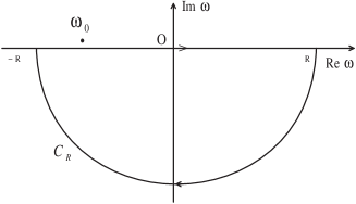
(a) The contour used for $t<t^{\prime}$. No poles is surrounded by the contour.

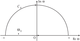
(b) The contour used for $t>t^{\prime}$. Only one pole $\omega_{0}$ is surrounded by the contour.

Figure 1: The contour used to calculate the integral in Eq. (15). $C_{R}$ is a semi-circular with radius $R$ ($R\rightarrow+\infty$).

Let us consider the $\omega$ integration in the complex $\omega$ plane,

$$\int^{+\infty}_{-\infty}\frac{\text{e}^{i\omega(t-t^{\prime})}}{\hslash\omega+D_{\alpha}|\mathrm{\textbf{p}}|^{\alpha}}\mathrm{d}\omega.$$ (15)

For the integrand, there is a pole on the path of integration at $\omega_{0}=-D_{\alpha}|\mathrm{\textbf{p}}|^{\alpha}/\hslash$. Considering the causality condition (5), this integration should be changed into

$$\int^{+\infty}_{-\infty}\frac{\text{e}^{i\omega(t-t^{\prime})}}{\hslash\omega+D_{\alpha}|\mathrm{\textbf{p}}|^{\alpha}-i\varepsilon}\mathrm{d}\omega,$$ (16)

where $\varepsilon$ is a positive infinitesimal [25]. Then the pole is removed to the upper half plane. For $t<t^{\prime}$, we use the contour shown in Fig. 1(a) to carry out the contour integral. Because no singularities lies inside the contour, the integral is zero, which means the causality condition is satisfied. For $t>t^{\prime}$, when we close the contour in the upper half-plane, as shown in Fig. 1(b), we get the contribution from the pole at $\omega_{0}$, and the result is

$$\lim_{\varepsilon\rightarrow 0^{+}}\int^{+\infty}_{-\infty}\frac{\text{e}^{i\omega(t-t^{\prime})}}{\hslash\omega+D_{\alpha}|\mathrm{\textbf{p}}|^{\alpha}-i\varepsilon}\mathrm{d}\omega=2\pi i\cdot\mbox{Res}\left\{\frac{\text{e}^{i\omega(t-t^{\prime})}}{\hslash\omega+D_{\alpha}|\mathrm{\textbf{p}}|^{\alpha}},\omega_{0}\right\}=\frac{2\pi i}{\hslash}\text{e}^{-iD_{\alpha}|\mathrm{\textbf{p}}|^{\alpha}(t-t^{\prime})/\hslash}.$$ (17)

Here, $\mbox{Res}\left\{*,\omega_{0}\right\}$ denotes the residue [26] of $*$ at $\omega_{0}$. Now Eq. (14) becomes

$$G(\mathrm{\textbf{r}},t;\mathrm{\textbf{r}}^{\prime},t^{\prime})=\frac{1}{(2\pi\hslash)^{2}\hslash i}\int\text{e}^{i\mathrm{\textbf{p}}\cdot(\mathrm{\textbf{r}}-\mathrm{\textbf{r}^{\prime}})/\hslash}\text{e}^{-iD_{\alpha}|\mathrm{\textbf{p}}|^{\alpha}(t-t^{\prime})/\hslash}\mathrm{d}^{2}\mathrm{\textbf{p}},\quad t>t^{\prime}.$$ (18)

To execute the above integration, we choose the polar coordinates $(p,\theta)$, with the positive direction of the $p$-axis along $\mathrm{\textbf{r}}-\mathrm{\textbf{r}}^{\prime}$. Then, $\mathrm{\textbf{p}}\cdot(\mathrm{\textbf{r}}-\mathrm{\textbf{r}^{\prime}})=p|\mathrm{\textbf{r}}-\mathrm{\textbf{r}^{\prime}}|\cos\theta$, in which $p$ and $|\mathrm{\textbf{r}}-\mathrm{\textbf{r}}^{\prime}|$ denote the magnitudes of the vectors p and $\mathrm{\textbf{r}}-\mathrm{\textbf{r}}^{\prime}$, respectively. Thus, Eq. (18) is converted into

$$\begin{split}G(\mathrm{\textbf{r}},t;\mathrm{\textbf{r}}^{\prime},t^{\prime})=\frac{1}{(2\pi\hslash)^{2}\hslash i}\int^{2\pi}_{0}\mathrm{d}\theta\int^{+\infty}_{0}\text{e}^{ip|\mathrm{\textbf{r}}-\mathrm{\textbf{r}^{\prime}}|\cos\theta/\hslash}\text{e}^{-iD_{\alpha}p^{\alpha}(t-t^{\prime})/\hslash}p\mathrm{d}p.\end{split}$$ (19)

Calculating the integral for $\theta$ yields

$$\int^{2\pi}_{0}\text{e}^{ip|\mathrm{\textbf{r}}-\mathrm{\textbf{r}^{\prime}}|\cos\theta/\hslash}\mathrm{d}\theta=2\int^{\pi}_{0}\cos({ip|\mathrm{\textbf{r}}-\mathrm{\textbf{r}^{\prime}}|\cos\theta/\hslash})\mathrm{d}\theta=2\pi J_{0}(p|\mathrm{\textbf{r}}-\mathrm{\textbf{r}^{\prime}}|/\hslash),$$ (20)

where $J_{0}(r)$ is the Bessel function of the first kind of order $0$. Furthermore, taking into account the series form of the Bessel function of the first kind of order $\nu$, that is,

$$\begin{split}J_{\nu}(z)=\frac{z^{\nu}}{2^{\nu}}\sum^{\infty}_{k=0}\frac{(-1)^{k}z^{2k}}{2^{2k}k!\Gamma\left(\nu+k+1\right)},\end{split}$$ (21)

we obtain

$$\begin{split}G(\mathrm{\textbf{r}},t;\mathrm{\textbf{r}}^{\prime},t^{\prime})=\frac{2\pi}{(2\pi\hslash)^{2}\hslash i}\sum^{\infty}_{k=0}\frac{(-1)^{k}(|\mathrm{\textbf{r}}-\mathrm{\textbf{r}^{\prime}}|/\hslash)^{2k}}{2^{2k}(k!)^{2}}I_{k},\end{split}$$ (22)

in which

$$I_{k}=\int^{+\infty}_{0}p^{2k+1}\text{e}^{-iD_{\alpha}p^{\alpha}(t-t^{\prime})/\hslash}\mathrm{d}p.$$ (23)

Making substitution $\tilde{p}=[D_{\alpha}(t-t^{\prime})/\hslash]^{1/\alpha}p\equiv\xi\cdot p$ gives

$$I_{k}=\xi^{-(2k+2)}\int^{+\infty}_{0}p^{2k+1}\text{e}^{-ip^{\alpha}}\mathrm{d}p,$$ (24)

in which $\tilde{p}$ has been replaced by $p$ for simplicity.

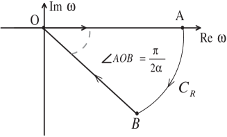
Figure 2: The contour used to calculate the integral in Eq. (24).

Then using the contour in Fig. 2, the above integral can be calculated.

$$\int^{+\infty}_{0}p^{2k+1}\text{e}^{-ip^{\alpha}}\mathrm{d}p=\frac{1}{\alpha}\Gamma(\frac{2k+2}{\alpha})\mbox{e}^{-\frac{k+1}{\alpha}\pi i}.$$ (25)

Finally, we obtain the Green’s function for the fractional Schrödinger equation in a series form,

$$G(\mathrm{\textbf{r}},t;\mathrm{\textbf{r}}^{\prime},t^{\prime})=\frac{\xi^{-2}}{2\alpha\pi\hslash^{3}i}\sum^{\infty}_{k=0}\frac{(-1)^{k}}{(k!)^{2}}\left[\frac{|\mathrm{\textbf{r}}-\mathrm{\textbf{r}^{\prime}}|}{2\xi\hslash}\right]^{2k}\Gamma(\frac{2k+2}{\alpha})\mbox{e}^{-\frac{k+1}{\alpha}\pi i},$$ (26)

in which $\xi=[D_{\alpha}(t-t^{\prime})/\hslash]^{1/\alpha}$. It can be proved that this Green’s function reduces to the one in the standard quantum mechanics when $\alpha=2$.

3 Time-independent Case

When the potential is independent of $t$, that is, $V(\mathrm{\textbf{r}},t)=V(\mathrm{\textbf{r}})$, after separation of variables, the steady state form of the fractional Schrödinger equation (1) can be obtained [19]:

$$-D_{\alpha}(\hslash\nabla)^{\alpha}\phi(\mathrm{\textbf{r}})+V(\mathrm{\textbf{r}})\phi(\mathrm{\textbf{r}})=E\phi(\mathrm{\textbf{r}}),$$ (27)

where $\phi(\mathrm{\textbf{r}})$ is related to $\psi(\mathrm{\textbf{r}},t)$ by $\psi(\mathrm{\textbf{r}},t)=\phi(\mathrm{\textbf{r}})\mbox{e}^{-iEt/\hslash}$ , in which $E$ denotes the energy of the quantum system.
Eq. (27) can be rewritten as

$$[(\hslash\nabla)^{\alpha}+\kappaup]\phi(\mathrm{\textbf{r}})=Q,$$ (28)

where $\kappaup=E/D_{\alpha}$,$Q=V\phi/D_{\alpha}$. Now, we define the Green’s function of the above equation by

$$[(\hslash\nabla)^{\alpha}+\kappaup]G(\mathrm{\textbf{r}})=\delta^{2}(\textbf{r}),$$ (29)

then $\phi$ can be expressed as:

$$\phi(\mathrm{\textbf{r}})=\phi_{0}(\mathrm{\textbf{r}})+\int G(\mathrm{\textbf{r}}-\mathrm{\textbf{r}}_{0})Q(\mathrm{\textbf{r}}_{0})\mathrm{d}^{2}\mathrm{\textbf{r}}_{0},$$ (30)

where $\phi_{0}(\mathrm{\textbf{r}})$ satisfies the free-particle Schrödinger equation,

$$[(\hslash\nabla)^{\alpha}+\kappaup]\phi_{0}(\mathrm{\textbf{r}})=0.$$ (31)

It is easy to prove that the basic solution to Eq. (31) is

$$\phi_{0}(\mathrm{\textbf{r}})=e^{i\mathrm{\textbf{k}}\cdot\mathrm{\textbf{r}}},\mbox{ {} {} (a constant product factor is omitted )}$$ (32)

where $\mathrm{\textbf{k}}=(K_{x},K_{y}),$ and $|\mathrm{\textbf{k}}|=\sqrt{K_{x}^{2}+K_{y}^{2}}=\kappaup^{1/\alpha}/\hslash$.
Now we turn back to solve Eq. (29). Defining

$$\hat{G}(\mathrm{\textbf{p}})=\int\mbox{e}^{-i\mathrm{\textbf{p}}\cdot\mathrm{\textbf{r}}/\hslash}G(\mathrm{\textbf{r}})\mathrm{d}^{2}\mathrm{\textbf{r}},\mbox{ and }G(\mathrm{\textbf{r}})=\frac{1}{(2\pi\hslash)^{2}}\int\mbox{e}^{i\mathrm{\textbf{p}}\cdot\mathrm{\textbf{r}}/\hslash}\hat{G}(\mathrm{\textbf{p}})\mathrm{d}^{2}\mathrm{\textbf{p}},$$ (33)

after taking the Fourier transform, Eq. (29) is changed into

$$[\kappaup-|\mathrm{\textbf{p}}|^{\alpha}]\hat{G}(\mathrm{\textbf{p}})=1,$$ (34)

That is,

$$\hat{G}(\mathrm{\textbf{p}})=\frac{1}{\kappaup-|\mathrm{\textbf{p}}|^{\alpha}}.$$ (35)

Inverting the Fourier transform gives

$$G(\mathrm{\textbf{r}})=\frac{1}{(2\pi\hslash)^{2}}\int\frac{\mbox{e}^{i\mathrm{\textbf{p}}\cdot\mathrm{\textbf{r}}/\hslash}}{\kappaup-|\mathrm{\textbf{p}}|^{\alpha}}\mathrm{d}^{2}\mathrm{\textbf{p}}.$$ (36)

To calculate the integral in the above formula, more work is needed. Denoting the magnitude of the vectors p and r by $p$ and $r$, respectively, with the help of the polar coordinates $(p,\theta)$, Eq. (36) can be converted into

$$G(\mathrm{\textbf{r}})=\frac{1}{(2\pi\hslash)^{2}}\int^{2\pi}_{0}\mathrm{d}\theta\int^{+\infty}_{0}\frac{\mbox{e}^{ipr\cos\theta/\hslash}}{\kappaup-p^{\alpha}}p\mathrm{d}p=\frac{1}{(\pi\hslash)^{2}}\int^{\pi/2}_{0}\mathrm{d}\theta\int^{+\infty}_{0}\frac{\cos({pr\cos\theta/\hslash})}{\kappaup-p^{\alpha}}p\mathrm{d}p.$$ (37)

When considering the quantum scattering problems, the energy of the quantum system satisfies $E>0$, that is, $\kappaup>0$. To evaluate the integral in Eq. (37), we should consider the quantum mechanics effect, and define two integrals, for the outgoing wave and the incoming wave respectively, as follows:

$$G^{\pm}(\mathrm{\textbf{r}})=\frac{1}{(\pi\hslash)^{2}}\int^{\pi/2}_{0}\mathrm{d}\theta\int^{+\infty}_{0}\frac{\cos({pr\cos\theta/\hslash})}{\kappaup-p^{\alpha}\pm i\varepsilon}p\mathrm{d}p,$$ (38)

where $\varepsilon$ is a positive infinitesimal (This manner can be called the “$i\varepsilon$ prescription”, see [21]). Note that in the quantum scattering problems, one is usually interested in the outgoing wave with $G^{+}(\mathrm{\textbf{r}})$ being considered. From Eqs. (38), we know $G^{-}(\mathrm{\textbf{r}})=[G^{+}(\mathrm{\textbf{r}})]^{*}$, and $G(\mathrm{\textbf{r}})=[G^{+}(\mathrm{\textbf{r}})+G^{-}(\mathrm{\textbf{r}})]/2$, so we only need to calculate $G^{+}(\mathrm{\textbf{r}})$ here. Substituting $p$ for $p/\kappaup^{1/\alpha}$ in Eq. (38) yields

$$G^{+}(\mathrm{\textbf{r}})=\frac{1}{(\pi\hslash)^{2}}\int^{\pi/2}_{0}\mathrm{d}\theta\int^{+\infty}_{0}\frac{\cos({p\kappaup^{1/\alpha}r\cos\theta/\hslash})}{1-p^{\alpha}+i\eta}p\mathrm{d}p,$$ (39)

where $\eta=\varepsilon/\kappaup$. Moreover, $G^{+}(\mathrm{\textbf{r}})$ can be rewritten as

$$G^{+}(\mathrm{\textbf{r}})=\frac{\kappaup^{(2-\alpha)/\alpha}}{2(\pi\hslash)^{2}}[I_{1}(r\kappaup^{1/\alpha}/\hslash)+I_{2}(r\kappaup^{1/\alpha}/\hslash)],$$ (40)

in which the two functions $I_{1}(r)$ and $I_{1}(r)$ are defined as

$$I_{1}(r)=\int^{\pi/2}_{0}\mathrm{d}\theta\int^{+\infty}_{0}\frac{pe^{ipr\cos\theta}}{1-p^{\alpha}+i\eta}\mathrm{d}p,$$ (41)

and

$$I_{2}(r)=\int^{\pi/2}_{0}\mathrm{d}\theta\int^{+\infty}_{0}\frac{pe^{-ipr\cos\theta}}{1-p^{\alpha}+i\eta}\mathrm{d}p.$$ (42)

The integral for $p$ can be evaluated by. To calculate the two integral, we can make use of the contour integral method and the residue theorem. It should be noted that all of the integrals in this paper take the Cauchy principal values. For $I_{1}(r)$, the contour is chosen as shown in Fig. 3.

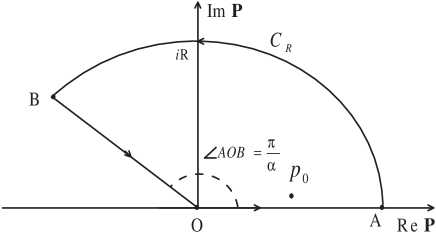
Figure 3: The contour used to calculate $I_{1}(r)$. $C_{R}=\stackrel{{\scriptstyle\frown}}{{AB}}$ is a circular segment with radius $R$. Only one pole $p_{0}$ is surrounded by the contour.

Note that in the definition of $G^{+}(\mathrm{\textbf{r}})$ in Eq. (38), the pole has been removed from the real axis to the upper half plane. There is one pole to be considered, $p_{0}=r_{\eta}e^{i\theta_{\eta}}$, in which $r_{\eta},\theta_{\eta}>0$, and $r_{\eta}\rightarrow 1$, $\theta_{\eta}\rightarrow 0$ as $\eta\rightarrow 0^{+}$, and the expression of $r_{\eta}$ and $\theta_{\eta}$ needs not be specified here. On the circular segment $C_{R}$, the formula

$$\lim\limits_{R\rightarrow+\infty}\frac{p}{1-p^{\alpha}}=0,(1<\alpha\leq 2)$$

holds uniformly, so according to the Jordan’s lemma [26], the integral

$$\int_{C_{R}}\frac{p\mbox{e}^{ipr\cos\theta}}{1-p^{\alpha}}\mathrm{d}p$$

is zero when $R\rightarrow+\infty$. Therefore, we have

$$I_{1}(r) =\lim\limits_{\eta\rightarrow 0^{+}}\lim\limits_{R\rightarrow+\infty}\left\{2\pi i\cdot\mbox{Res}\Big{(}\frac{pe^{ipr\cos\theta}}{1-p^{\alpha}+i\eta};p_{0}\Big{)}-\Bigg{(}\int_{C_{R}}+\int_{\overrightarrow{BO}}\Bigg{)}\frac{pe^{ipr\cos\theta}}{1-p^{\alpha}+i\eta}\mathrm{d}p\right\}$$

$$=-\frac{2\pi i}{\alpha}e^{ir\cos\theta}+I_{\overrightarrow{OB}},$$ (43)

where

$$I_{\overrightarrow{OB}}=\lim\limits_{R\rightarrow+\infty}\int_{\overrightarrow{OB}}\frac{pe^{ipr\cos\theta}}{1-p^{\alpha}}\mathrm{d}p.$$ (44)

Taking into account that $p=\tilde{p}e^{\frac{\pi i}{\alpha}}$ ($\tilde{p}\geq 0$) on $\overrightarrow{OB}$, inserting this expression for $p$ into Eq. (44) gives

$$I_{\overrightarrow{OB}}=e^{\frac{2\pi i}{\alpha}}[\mathbb{I}_{1}(r,\theta)+i\cdot\mathbb{I}_{2}(r,\theta)],$$ (45)

where

$$\mathbb{I}_{1}(r,\theta)=\int^{+\infty}_{0}\frac{p}{1+p^{\alpha}}e^{-\sin(\pi/\alpha)pr\cos\theta}\cos[\cos(\pi/\alpha)pr\cos\theta]\mathrm{d}p,$$ (46)

$$\mathbb{I}_{2}(r,\theta)=\int^{+\infty}_{0}\frac{p}{1+p^{\alpha}}e^{-\sin(\pi/\alpha)pr\cos\theta}\sin[\cos(\pi/\alpha)pr\cos\theta]\mathrm{d}p,$$ (47)

in which $\tilde{p}$ has been replaced by $p$ for simplicity. Therefore, we get

$$I_{1}(r) =\int^{\pi/2}_{0}\left\{-\frac{2\pi i}{\alpha}e^{ir\cos\theta}+e^{\frac{2\pi i}{\alpha}}[\mathbb{I}_{1}(r,\theta)+i\cdot\mathbb{I}_{2}(r,\theta)]\right\}\mathrm{d}\theta$$ (48)

$$=-\frac{2\pi i}{\alpha}\int^{\pi/2}_{0}e^{ir\cos\theta}\mathrm{d}\theta+e^{\frac{2\pi i}{\alpha}}[\mathcal{I}_{1}(r)+i\mathcal{I}_{2}(r)],$$ (49)

where

$$\mathcal{I}_{1}(r)=\int^{\pi/2}_{0}\mathbb{I}_{1}(r,\theta)\mathrm{d}\theta,\mbox{ and }\mathcal{I}_{2}(r)=\int^{\pi/2}_{0}\mathbb{I}_{2}(r,\theta)\mathrm{d}\theta.$$ (50)

In a similar way, $I_{2}(r)$ can also be calculated, and expressed in terms of $\mathcal{I}_{1}(r)$ and $\mathcal{I}_{2}(r)$. Note that there is no poles to be considered when calculating $I_{2}(r)$. The result is

$$I_{2}(r)=e^{-\frac{2\pi i}{\alpha}}[\mathcal{I}_{1}(r)-i\mathcal{I}_{2}(r)].$$ (51)

The first integral in Eq. (49) can be calculated as

$$\int^{\pi/2}_{0}e^{ir\cos\theta}\mathrm{d}\theta= \int^{\pi/2}_{0}\cos(r\cos\theta)\mathrm{d}\theta+i\int^{\pi/2}_{0}\sin(r\cos\theta)\mathrm{d}\theta$$ (52)

$$= \frac{\pi}{2}\left[J_{0}(r)+iH_{0}(r)\right],$$ (53)

where $J_{0}(r)$ is the Bessel function of the first kind of order $0$, and $H_{0}(r)$ is the Struve function of order $0$. The two integrals $\mathcal{I}_{1}(r)$ and $\mathcal{I}_{2}(r)$ in Eq. (50) can be expressed in terms of Fox’s H-function, using the Mellin transform and its inverse transform. With the help of the following formulas for the Mellin transform (see P.1189 of [27])

$$\mathcal{M}\mbox{ }\Big{\{}e^{-ax}\sin(bx),s\Big{\}}=\frac{\Gamma(s)\sin[s\arctan\cot(b/a)]}{(a^{2}+b^{2})^{s/2}},\quad a>0,\mbox{ Re }s>-1$$ (54)

$$\mathcal{M}\mbox{ }\Big{\{}e^{-ax}\cos(bx),s\Big{\}}=\frac{\Gamma(s)\cos[s\arctan\cot(b/a)]}{(a^{2}+b^{2})^{s/2}},\quad a>0,\mbox{ Re }s>0$$ (55)

and considering the formula (see formula 3.241.2 of [28]),

$$\int^{+\infty}_{0}\frac{x^{a-1}}{x^{b}+1}\mathrm{d}x=\frac{\pi}{b}\csc(\frac{a}{b}\pi),\qquad\mbox{ Re }b>\mbox{ Re }a>0$$ (56)

the Mellin transform of $\mathcal{I}_{1}(r)$ and $\mathcal{I}_{2}(r)$ can be calculated as

$$\tilde{\mathcal{I}}_{1}(s) =\mathcal{M}\mbox{ }\Big{\{}\mathcal{I}_{1}(r),s\Big{\}}=\int^{\pi/2}_{0}\mathcal{M}\mbox{ }\Big{\{}\mathbb{I}_{1}(r,\theta),s\Big{\}}\mathrm{d}\theta$$ (57)

$$=\Gamma(s)\cos(\lambda\pi s)\cdot\int^{\pi/2}_{0}(\cos\theta)^{-s}\mathrm{d}\theta\cdot\int^{+\infty}_{0}\frac{p^{1-s}}{1+p^{\alpha}}\mathrm{d}p$$ (58)

$$=\frac{\pi}{\alpha}\frac{\Gamma(s)\cos(\lambda\pi s)}{2^{s+1}\sin(\frac{2-s}{\alpha}\pi)}\beta\left(\frac{1-s}{2},\frac{1-s}{2}\right)=\frac{\pi}{\alpha}\frac{\Gamma(s)\Gamma(1-\frac{2-s}{\alpha})\Gamma(\frac{1-s}{2})\Gamma(\frac{1-s}{2})\Gamma(\frac{2-s}{\alpha})}{2^{s+1}\Gamma(\frac{1}{2}+\lambda s)\Gamma(1-s)\Gamma(\frac{1}{2}-\lambda s)},$$

$$\tilde{\mathcal{I}}_{2}(s)=\mathcal{M}\mbox{ }\Big{\{}\mathcal{I}_{2}(r),s\Big{\}}=\int^{\pi/2}_{0}\mathcal{M}\mbox{ }\Big{\{}\mathbb{I}_{2}(r,\theta),s\Big{\}}\mathrm{d}\theta=-\frac{\pi}{\alpha}\frac{\Gamma(s)\Gamma(1-\frac{2-s}{\alpha})\Gamma(\frac{1-s}{2})\Gamma(\frac{1-s}{2})\Gamma(\frac{2-s}{\alpha})}{2^{s+1}\Gamma(\lambda s)\Gamma(1-s)\Gamma(1-\lambda s)},$$ (59)

where $\lambda=-\arctan[\cot(\pi/\alpha)]/\pi$, and $0\leq\lambda<1/2$ when $1<\alpha\leq 2$. Additionally, $\lambda=0$ only when $\alpha=2$, and at that time, $\tilde{\mathcal{I}_{2}}(s)\equiv 0$, so that $\mathcal{I}_{2}(r)\equiv 0$. Inverting the Mellin transform, and comparing the expression with the definition of the Fox’s H-function, we obtain

$$\mathcal{I}_{1}(r)=\frac{1}{2\pi i}\int^{c+i\infty}_{c-i\infty}r^{-s}\tilde{\mathcal{I}}_{1}(s)\mathrm{d}s=\frac{\pi}{2\alpha}H^{2,3}_{4,4}\left[2r\mbox{ }\Bigg{|}\begin{aligned} &{\mbox{ }(1/2,1/2),(1/2,1/2),(1-2/\alpha,1/\alpha),(1/2,\lambda)}\\ &{\mbox{ }(0,1),(1-2/\alpha,1/\alpha),(0,1),(1/2,\lambda)}\end{aligned}\right]\equiv\frac{\pi}{2\alpha}\mathscr{H}_{1}(r),$$ (60)

$$\mathcal{I}_{2}(r)=\frac{1}{2\pi i}\int^{c+i\infty}_{c-i\infty}r^{-s}\tilde{\mathcal{I}}_{2}(s)\mathrm{d}s=-\frac{\pi}{2\alpha}H^{2,3}_{4,4}\left[2r\mbox{ }\Bigg{|}\begin{aligned} &{\mbox{ }(1/2,1/2),(1/2,1/2),(1-2/\alpha,1/\alpha),(0,\lambda)}\\ &{\mbox{ }(0,1),(1-2/\alpha,1/\alpha),(0,1),(0,\lambda)}\end{aligned}\right]\equiv-\frac{\pi}{2\alpha}\mathscr{H}_{2}(r).$$ (61)

Finally, using the results in Eqs. (49), (51), (60) and (61), from Eq. (40), the Green’s function $G^{+}(r)$ for the outgoing wave can be calculated in terms of the Bessel function, Struve function and Fox’s H-function as:

$$G^{+}(\mathrm{\textbf{r}})=\frac{\kappaup^{(2-\alpha)/\alpha}}{2\alpha\hslash^{2}i}\left[J_{0}(r\kappaup^{1/\alpha}/\hslash)+iH_{0}(r\kappaup^{1/\alpha}/\hslash)\right]+\frac{\kappaup^{(2-\alpha)/\alpha}}{2\alpha\pi\hslash^{2}}\mathcal{G}(r\kappaup^{1/\alpha}/\hslash),$$ (62)

where

$$\mathcal{G}(r)=\cos{\frac{2\pi}{\alpha}}\mathscr{H}_{1}(r)+\sin{\frac{2\pi}{\alpha}}\mathscr{H}_{2}(r).$$ (63)

4 Asymptotic properties of the Green’s functions and Applications to the Scattering Problems

In the scattering problems, we usually consider the behavior of the particles far away from the scattering center, and assume the potential $V(\mathrm{\textbf{r}})$ is non-zero only in a small domain. In this section, we discuss the asymptotic properties of the Green’s functions obtained in the previous sections, and then apply them to study the fractional scattering problems.

4.1 Time-dependent case]

To get the asymptotic formula for the Green’s function, we can rewritten it in terms of the H-function. The formula of the Green’s function can be rewritten as,

$$\begin{split}G(\mathrm{\textbf{r}},t;\mathrm{\textbf{r}}^{\prime},t^{\prime})&=\frac{\xi^{-2}}{2\alpha\pi\hslash^{3}i}\sum^{\infty}_{k=0}\frac{(-1)^{k}}{(k!)^{2}}\left(\frac{|\mathrm{\textbf{r}}-\mathrm{\textbf{r}^{\prime}}|}{2\xi\hslash}\right)^{2k}\Gamma(\frac{2k+2}{\alpha})\left(\cos\frac{k+1}{\alpha}\pi-i\sin\frac{k+1}{\alpha}\pi\right)\\ &=\frac{\xi^{-2}}{2\alpha\hslash^{3}i}\sum^{\infty}_{k=0}\left[\frac{\Gamma(\frac{2k+2}{\alpha})}{\Gamma(k+1)\Gamma(\frac{1}{2}+\frac{1}{\alpha}+\frac{k}{\alpha})\Gamma(\frac{1}{2}-\frac{1}{\alpha}-\frac{k}{\alpha})}-i\frac{\Gamma(\frac{2k+2}{\alpha})}{\Gamma(k+1)\Gamma(\frac{1}{\alpha}+\frac{k}{\alpha})\Gamma(1-\frac{1}{\alpha}-\frac{k}{\alpha})}\right]\frac{(-1)^{k}}{k!}y^{k},\end{split}$$ (64)

in which $y=\left(\frac{|\mathrm{\textbf{r}}-\mathrm{\textbf{r}^{\prime}}|}{2\xi\hslash}\right)^{2}$. Comparing this equation to the definition of Fox’s H-function, we can get that

$$G(\mathrm{\textbf{r}},t;\mathrm{\textbf{r}}^{\prime},t^{\prime})=\frac{\xi^{-2}}{2\alpha\hslash^{3}i}\left[\mathcal{H}_{1}(y)-i\mathcal{H}_{2}(y)\right]$$ (65)

in which

$$\mathcal{H}_{1}(y)=H^{1,1}_{2,3}\left[y\mbox{ }\Bigg{|}\begin{aligned} &{\mbox{ }(1-2/\alpha,2/\alpha),(1/2-1/\alpha,1/\alpha)}\\ &{\mbox{ }(0,1),(0,1),(1/2-1/\alpha,1/\alpha)}\end{aligned}\right],$$ (66)

$$\mathcal{H}_{2}(y)=H^{1,1}_{2,3}\left[y\mbox{ }\Bigg{|}\begin{aligned} &{\mbox{ }(1-2/\alpha,2/\alpha),(1-1/\alpha,1/\alpha)}\\ &{\mbox{ }(0,1),(0,1),(1-1/\alpha,1/\alpha)}\end{aligned}\right].$$ (67)

By use the asymptotic properties of H function, we can get

$$\begin{split}G(\mathrm{\textbf{r}},t;\mathrm{\textbf{r}}^{\prime},t^{\prime})&=2\pi iAy^{(\mu+1/2)/\Delta}\mbox{e}^{i(B+Cy^{1/\Delta}-\pi/\alpha)}+\mbox{o}(y^{(\mu+1/2)/\Delta}).\\ &=-\frac{|\mathrm{\textbf{r}}-\mathrm{\textbf{r}}^{\prime}|^{(2-\alpha)/(\alpha-1)}}{2\pi\hslash^{2}[\alpha D_{\alpha}(t-t^{\prime})]^{1/(\alpha-1)}\sqrt{\alpha-1}}\exp\left\{i\frac{\alpha-1}{\hslash}\left(\frac{|\mathrm{\textbf{r}}-\mathrm{\textbf{r}}^{\prime}|^{\alpha}}{\alpha^{\alpha}D_{\alpha}(t-t^{\prime})}\right)^{\frac{1}{\alpha-1}}\right\}+\mbox{o}\left(|\mathrm{\textbf{r}}-\mathrm{\textbf{r}}^{\prime}|^{\frac{2-\alpha}{\alpha-1}}\right)\end{split},$$ (68)

In the scattering problem, we can use merely the first term of the asymptotic formula (68) for $G(\mathrm{\textbf{r}},t;\mathrm{\textbf{r}}^{\prime},t^{\prime})$, then an approximate wave function for the scattering problem can be obtained. Let’s invoke the Born approximation [9, 33]: Suppose the incoming plane wave is not substantially altered by the potential. Then, in Eq. (6), it makes sense to use

$$\psi(\mathrm{\textbf{r}}^{\prime},t^{\prime})\approx\psi_{0}(\mathrm{\textbf{r}}^{\prime},t^{\prime})=e^{i(\mathrm{\textbf{k}}\cdot\mathrm{\textbf{r}}^{\prime}-Et^{\prime})/\hslash}.$$ (69)

Then Eq. (6) becomes

$$\begin{split}\psi(\mathrm{\textbf{r}},t)\approx\psi_{0}&(\mathrm{\textbf{r}},t)-\frac{(\alpha D_{\alpha})^{1/(1-\alpha)}}{2\pi\hslash^{2}\sqrt{\alpha-1}}\int\frac{|\mathrm{\textbf{r}}-\mathrm{\textbf{r}^{\prime}}|^{(2-\alpha)/(\alpha-1)}}{(t-t^{\prime})^{1/(\alpha-1)}}\exp\Bigg{\{}i\frac{\alpha-1}{\hslash}\left(\frac{|\mathrm{\textbf{r}}-\mathrm{\textbf{r}}^{\prime}|^{\alpha}}{\alpha^{\alpha}D_{\alpha}(t-t^{\prime})}\right)^{\frac{1}{\alpha-1}}+\\ &i(\mathrm{\textbf{k}}\cdot\mathrm{\textbf{r}}^{\prime}-Et^{\prime})/\hslash\Bigg{\}}V(\mathrm{\textbf{r}}^{\prime},t^{\prime})\mathrm{d}^{2}\mathrm{\textbf{r}}^{\prime}\mathrm{d}t^{\prime}.\end{split}$$ (70)

Further more, assuming the potential $V(\mathrm{\textbf{r}})$ is non-zero only in a small domain, then we have $|\mathrm{\textbf{r}}-\mathrm{\textbf{r}^{\prime}}|\approx|\mathrm{\textbf{r}}|=r$, we can get

$$\begin{split}\psi(\mathrm{\textbf{r}},t)\approx\psi_{0}&(\mathrm{\textbf{r}},t)-\frac{(\alpha D_{\alpha}r^{\alpha-2})^{\frac{1}{1-\alpha}}}{2\pi\hslash^{2}\sqrt{\alpha-1}}\int(t-t^{\prime})^{\frac{1}{1-\alpha}}\exp\Bigg{\{}i\frac{\alpha-1}{\hslash}\left(\frac{(r/\alpha)^{\alpha}}{D_{\alpha}(t-t^{\prime})}\right)^{\frac{1}{\alpha-1}}+i(\mathrm{\textbf{k}}\cdot\mathrm{\textbf{r}}^{\prime}-Et^{\prime})/\hslash\Bigg{\}}V(\mathrm{\textbf{r}}^{\prime},t^{\prime})\mathrm{d}^{2}\mathrm{\textbf{r}}^{\prime}\mathrm{d}t^{\prime}.\end{split}$$ (71)

The second term of the right side of the above formula gives the approximate scattering wave function.

We can also generate a series of higher-order corrections to the approximate wave function. From Eq. (6), we can build an iteration scheme for the wave function as

$$\psi^{(n)}(\mathrm{\textbf{r}},t)=\psi_{0}(\mathrm{\textbf{r}},t)+\int G(\mathrm{\textbf{r}},t;\mathrm{\textbf{r}}^{\prime},t^{\prime})V(\mathrm{\textbf{r}}^{\prime},t^{\prime})\psi^{(n-1)}(\mathrm{\textbf{r}}^{\prime},t^{\prime})\mathrm{d}^{3}\mathrm{\textbf{r}}^{\prime}\mathrm{d}t^{\prime}.$$ (72)

Note that $\phi^{(0)}(\mathrm{\textbf{r}},t)=\psi_{0}(\mathrm{\textbf{r}},t)=e^{i(\mathrm{\textbf{k}}\cdot\mathrm{\textbf{r}}-Et)/\hslash}$, and $\phi^{(n)}$ is the $n$th-order corrections to the wave function. For a given potential function, using Eq. (72), the analytical approximate solutions of every order can be obtained. In a series form, we have

$$\phi=\phi_{0}+\int GV\phi_{0}+\iint GVGV\phi_{0}+\iiint GVGVGV\phi_{0}+\cdots.$$ (73)

In each integrand only the incident wave function ($\phi_{0}$) appears, together with more and more powers of $GV$.

4.2 Time-independent case

For the Green’s function , for the the Bessel function and Struve function, we have the following asymptotic formulas,

$$H_{0}[r]=Y_{0}(r)+\mbox{O}(|r|^{-1}),Y_{0}(r)\sim\sqrt{\frac{2}{\pi r}}\sin[r-\frac{\pi}{4}],\mbox{ { } }r\rightarrow\infty,$$ (74)

$$J_{0}[r]\sim\sqrt{\frac{2}{\pi r}}\cos[r-\frac{\pi}{4}],\mbox{ when}r\rightarrow+\infty.$$ (75)

Meantime, with the help of the properties of the H function, we obtain the asymptotic formulas for the two H functions, $\mathscr{H}_{1}(r)$, and $\mathscr{H}_{2}(r)$,

$$\mathscr{H}_{1}(r),\mathscr{H}_{2}(r)=\mbox{o}\left(\frac{\log(r)}{r}\right),\mbox{ when}r\rightarrow+\infty.$$ (76)

Therefore, the Green’s function can be approximate to

$$\begin{split}G^{+}(\mathrm{\textbf{r}})&\sim\frac{\kappaup^{(2-\alpha)/\alpha}}{2\alpha\hslash^{2}i}\left[J_{0}(r\kappaup^{1/\alpha}/\hslash)+iY_{0}(r\kappaup^{1/\alpha}/\hslash)\right]\equiv\frac{\kappaup^{(2-\alpha)/\alpha}}{2\alpha\hslash^{2}i}H^{(1)}_{0}(r\kappaup^{1/\alpha}/\hslash)\\ &\sim\frac{\kappaup^{(2-\alpha)/\alpha}}{2\alpha\hslash^{2}i}\sqrt{\frac{2\hslash}{\pi\kappaup^{1/\alpha}r}}\exp[(r\kappaup^{1/\alpha}/\hslash-\frac{\pi}{4})i]\\ &=-\frac{\kappaup^{(3-2\alpha)/(2\alpha)}}{\alpha\sqrt{2\pi r\hslash^{3}}}e^{\frac{\pi}{4}i}\exp[ir\kappaup^{1/\alpha}/\hslash],\mbox{ when}r\rightarrow+\infty.\end{split}$$ (77)

In a similar way to the time-dependent case, using the first term of the above formula instead of the exact results for the Green’s function $G^{+}(\mathrm{\textbf{r}})$, the integral equation(30) can be simplified to

$$\phi(\mathrm{\textbf{r}})\cong\mbox{e}^{i\mathrm{\textbf{k}}\cdot\mathrm{\textbf{r}}}-\frac{\kappaup^{(3-2\alpha)/(2\alpha)}e^{\frac{\pi}{4}i}}{\sqrt{2\pi r\hslash^{3}}\alpha D_{\alpha}}\int{e^{i\kappaup^{1/\alpha}|\mathrm{\textbf{r}}-\mathrm{\textbf{r}}_{0}|/\hslash}}V(\mathrm{\textbf{r}}_{0})\phi(\mathrm{\textbf{r}}_{0})\mathrm{d}^{2}\mathrm{\textbf{r}}_{0}.$$ (78)

Meantime, we have

$$|\mathrm{\textbf{r}}-\mathrm{\textbf{r}}_{0}|=\sqrt{\mathrm{\textbf{r}}^{2}-2\mathrm{\textbf{r}}\cdot\mathrm{\textbf{r}}_{0}+\mathrm{\textbf{r}}_{0}^{2}}\cong r-\frac{\mathrm{\textbf{r}}\cdot\mathrm{\textbf{r}}_{0}}{r}.$$ (79)

Substituting $|\mathrm{\textbf{r}}-\mathrm{\textbf{r}}_{0}|$ by Eq. (79) in Eq. (78) yields

$$\phi(\mathrm{\textbf{r}})\cong\phi_{0}(\mathrm{\textbf{r}})-\frac{\kappaup^{3/(2\alpha)-1}\mbox{e}^{i(\kappaup^{1/\alpha}r/\hslash+\pi/4)}}{\sqrt{2\pi r\hslash^{3}}\alpha D_{\alpha}}\int\mbox{e}^{-i\mathrm{\textbf{k}}_{f}\cdot\mathrm{\textbf{r}}_{0}}V(\mathrm{\textbf{r}}_{0})\phi(\mathrm{\textbf{r}}_{0})\mathrm{d}^{2}\mathrm{\textbf{r}}_{0},$$ (80)

where

$$\mathrm{\textbf{k}}_{f}=\frac{\kappaup^{1/\alpha}}{\hslash}\frac{\mathrm{\textbf{r}}}{r}.$$ (81)

Now we invoke the Born approximation [21, 33]: Suppose the incoming plane wave is not substantially altered by the potential. Then, in Eq. (78), it makes sense to use

$$\phi(\mathrm{\textbf{r}}_{0})\approx\phi_{0}(\mathrm{\textbf{r}}_{0})=\mbox{e}^{i\mathrm{\textbf{k}}\cdot\mathrm{\textbf{r}}_{0}},$$ (82)

which yields

$$\phi(\mathrm{\textbf{r}})\approx\mbox{e}^{i\mathrm{\textbf{k}}\cdot\mathrm{\textbf{r}}}-\frac{\kappaup^{3/(2\alpha)-1}\mbox{e}^{i(\kappaup^{1/\alpha}r/\hslash+\pi/4)}}{\sqrt{2\pi r\hslash^{3}}\alpha D_{\alpha}}\int\mbox{e}^{-i\mathrm{\textbf{q}}\cdot\mathrm{\textbf{r}}_{0}}V(\mathrm{\textbf{r}}_{0})\mathrm{d}^{3}\mathrm{\textbf{r}}_{0},$$ (83)

where $\mathrm{\textbf{q}}=\mathrm{\textbf{k}}_{f}-\mathrm{\textbf{k}}$. Here, vector k points in the incident direction, $\mathrm{\textbf{k}}_{f}$ in the scattered direction, and they both have magnitude $\kappaup^{1/\alpha}/\hslash$. Therefore, $q=|\mathrm{\textbf{q}}|=2\kappaup^{1/\alpha}sin(\theta/2)/\hslash$, where $\theta$ is the scattering angle, the angle between $\mathrm{\textbf{k}}_{f}$ and k. So, $\hslash\mathrm{\textbf{q}}$ is the momentum transfer in the process [8, 21]. Eq. (83) gives the approximate wave function of the fractional quantum scattering problem, and the second term of the right side of this equation denotes the scattering wave.

In the zeroth-order Born approximation the incident plane wave passes by with no modification, and what we explored in Eq. (83) can be viewed as the first-order correction to this. We can also generate a series of higher-order corrections: the Born series [21, 33]. The generalized Lippmann-Schwinger equation (LABEL:lsequation1) can be written as

$$\phi(\mathrm{\textbf{r}})=\phi_{0}(\mathrm{\textbf{r}})+\int g(\mathrm{\textbf{r}}-\mathrm{\textbf{r}}_{0})V(\mathrm{\textbf{r}}_{0})\phi(\mathrm{\textbf{r}}_{0})\mathrm{d}^{3}\mathrm{\textbf{r}}_{0},$$ (84)

where $g(\mathrm{\textbf{r}})=G^{+}(\mathrm{\textbf{r}})/D_{\alpha}.$ We can build an iteration scheme for the wave function as

$$\phi^{(n)}=\mbox{e}^{i\mathrm{\textbf{k}}\cdot\mathrm{\textbf{r}}}+\int g(\mathrm{\textbf{r}}-\mathrm{\textbf{r}}_{0})V(\mathrm{\textbf{r}}_{0})\phi^{(n-1)}(\mathrm{\textbf{r}}_{0})\mathrm{d}^{3}\mathrm{\textbf{r}}_{0}.$$ (85)

Note that $\phi^{(0)}=\mbox{e}^{i\mathrm{\textbf{k}}\cdot\mathrm{\textbf{r}}}$, and $\phi^{(n)}$ is the $n$th-order corrections to the wave function. For a given potential function, using Eq. (85), the analytical approximate solutions of every order can be obtained. In a series form, we have

$$\phi=\phi_{0}+\int gV\phi_{0}+\iint gVgV\phi_{0}+\iiint gVgVgV\phi_{0}+\cdots.$$ (86)

In each integrand only the incident wave function ($\phi_{0}$) appears, together with more and more powers of $gV$.

5 Conclusions

In this paper, the 2D space-FSE with time-dependent and time-independent potentials was studied. We defined the Green’s function of the FSE for the fractional scattering problem in the two cases, and the FSE was converted into an integral form. We gave the mathematical expression of the Green’s function in terms of some special functions. The asymptotic properties of the Green’s functions for $|\mathrm{\textbf{r}}-\mathrm{\textbf{r}}^{\prime}|\rightarrow\infty$ (or $|\mathrm{\textbf{r}}|>>|\mathrm{\textbf{r}}^{\prime}|$) were also given. Using these results, we obtained the approximate scattering wave function for the fractional quantum scattering problems (see Eqs. (71) and (83)). A series of higher-order corrections to the approximate wave functions were also given in Eqs. (72) and (85). These results are useful for the time-dependent scattering problem in the fractional quantum mechanics. All of these results contain those in the standard quantum mechanics as special cases.

Appendix Appendix: Fox’s $H$-function and Some Properties

The Fox’s $H$-function [29, 30] is defined by an integral of Mellin-Barnes type [34] as

$$H^{m,n}_{p,q}(z)=H^{m,n}_{p,q}\left[z\text{ }\Bigg{|}\begin{aligned} &{\text{ }(a_{1},A_{1}),(a_{2},A_{2}),\ldots,(a_{p},A_{p})}\\ &{\text{ }(b_{1},B_{1}),(b_{2},B_{2}),\ldots,(b_{p},B_{p})}\end{aligned}\right]=\cfrac{1}{2\pi i}\int_{L}\chi(s)z^{-s}\mathrm{d}s,$$ (A1)

where

$$\chi(s)=\cfrac{\prod^{m}_{j=1}\Gamma(b_{j}+B_{j}s)\prod^{n}_{i=1}\Gamma(1-a_{i}-A_{i}s)}{\prod^{p}_{i=n+1}\Gamma(a_{i}+A_{i}s)\prod^{q}_{j=m+1}\Gamma(1-b_{j}-B_{j}s)}.$$ (A2)

The contour $L$ runs from $c-i\infty$ to $c+i\infty$ separating the poles of $\Gamma(1-a_{i}-A_{i}s)$, ($i=1,\cdots,n$) from those of $\Gamma(b_{j}+B_{j}s)$, ($j=1,\cdots,m$). Here we present some properties of the $H$-function used in our paper. In order to give the results, the following definitions will be used,

$$\Delta=\sum^{q}_{j=1}B_{j}-\sum^{p}_{i=1}A_{j};\quad\Delta^{*}=\sum^{n}_{i=1}A_{i}-\sum^{p}_{i=n+1}A_{i}+\sum^{m}_{j=1}B_{j}-\sum^{q}_{j=m+1}B_{j};$$ (A3)

$$\delta=\prod^{p}_{j=1}(A_{j})^{-A_{j}}\prod^{q}_{j=1}(B_{j})^{B_{j}};\quad\mu=\sum^{q}_{j=1}b_{j}-\sum^{p}_{i=1}a_{i}+\frac{p-q}{2}.$$

The following properties of the $H$-function can be found in Refs. [30, 29, 31].
Property 1:

$$\frac{1}{k}H^{m,n}_{p,q}\left[z\text{ }\Bigg{|}\begin{aligned} &{\text{ }(a_{p},A_{p})}\\ &{\text{ }(b_{p},B_{p}))}\end{aligned}\right]=H^{m,n}_{p,q}\left[z^{k}\text{ }\Bigg{|}\begin{aligned} &{\text{ }(a_{p},kA_{p})}\\ &{\text{ }(b_{p},kB_{p})}\end{aligned}\right].\quad\mbox{for }k>0$$ (A4)

Property 2:

$$z^{\sigma}H^{m,n}_{p,q}\left[z\text{ }\Bigg{|}\begin{aligned} &{\text{ }(a_{p},A_{p})}\\ &{\text{ }(b_{p},B_{p}))}\end{aligned}\right]=H^{m,n}_{p,q}\left[z\text{ }\Bigg{|}\begin{aligned} &{\text{ }(a_{p}+\sigma A_{p},A_{p})}\\ &{\text{ }(b_{p}+\sigma B_{p},B_{p})}\end{aligned}\right].\quad\mbox{for }\sigma\in\mathbb{C}$$ (A5)

Property 3: Explicit Power Series Expansion

For $\Delta>0$ , $z\neq 0$ or $\Delta=0$, $|z|>\delta$, there holds the following expansion for the $H$-function [30],

$$H^{m,n}_{p,q}(z)=\sum^{m}_{h=1}\sum^{\infty}_{k=0}\cfrac{\prod^{m}_{j=1,j\neq h}\Gamma(b_{j}-B_{j}s_{hk})\prod^{n}_{i=1}\Gamma(1-a_{i}+A_{i}s_{hk})}{\prod^{p}_{i=n+1}\Gamma(a_{i}-A_{i}s_{hk})\prod^{q}_{j=m+1}\Gamma(1-b_{j}+B_{j}s_{hk})}\frac{(-1)^{k}}{k!}\frac{z^{s_{hk}}}{B_{h}},$$ (A6)

where $s_{hk}=(b_{h}+k)/B_{h}$, if the following conditions are satisfied:

1. The poles of the gamma functions $\Gamma(1-a_{i}-A_{i}s)$, ($i=1,\cdots,n$) and those of $\Gamma(b_{j}+B_{j}s)$, ($j=1,\cdots,m$) do not coincide:

   $$A_{i}(b_{j}+l)\neq B_{j}(a_{i}-k-1),(i=1,\cdots,n;j=1,\cdots,m;k,l=0,1,2,\cdots).$$ (A7)

2. The poles of the gamma functions $\Gamma(b_{j}+B_{j}s)$, ($j=1,\cdots,m$) are simple:

   $$B_{i}(b_{j}+l)\neq B_{j}(b_{i}+k),(i\neq j;i,j=1,\cdots,m;k,l=0,1,2,\cdots).$$ (A8)

Property 4: Asymptotic Expansions at Infinity in the Case $\Delta>0$, $\Delta^{*}=0$

When the poles of the gamma functions $\Gamma(1-a_{i}-A_{i}s)$, ($i=1,\cdots,n$) are simple:

$$A_{i}(1-A_{j}+l)\neq A_{j}(1-a_{i}+k),(i\neq j;i,j=1,\cdots,n;k,l=0,1,2,\cdots),$$ (A9)

and the condition (A7) is satisfied, the $H$-function has the following asymptotic expansion [2, 31],

$$\begin{split}H^{m,n}_{p,q}(z)=&\sum^{n}_{i=1}\left[h_{i}z^{(a_{i}-1)/A_{i}}+\mbox{o}\left(z^{(a_{i}-1)/A_{i}}\right)\right]+Az^{(\mu+1/2)/\Delta}\Big{(}c_{0}\exp\left[(B+Cz^{1/\Delta})i\right]-\\ &d_{0}\exp\left[-(B+Cz^{1/\Delta})i\right]\Big{)}+\mbox{o}\left(z^{(\mu+1/2)/\Delta}\right),\end{split}$$ (A10)

where

$$h_{i}=\frac{1}{A_{i}}\cfrac{\prod^{m}_{j=1}\Gamma(b_{j}-B_{j}(a_{i}-1)/A_{i})\prod^{n}_{j=1,j\neq i}\Gamma(1-a_{j}+A_{j}(a_{i}-1)/A_{i})}{\prod^{p}_{j=n+1}\Gamma(a_{j}-A_{j}(a_{i}-1)/A_{i})\prod^{q}_{j=m+1}\Gamma(1-b_{j}+B_{j}(a_{i}-1)/A_{i})},$$ (A11)

$$A=\frac{A_{0}}{2\pi i\Delta}\left(\frac{\Delta^{\Delta}}{\delta}\right)^{(\mu+1/2)/\Delta},\quad B=\frac{(2\mu+1)\pi}{4},\quad C=\left(\frac{\Delta^{\Delta}}{\delta}\right)^{1/\Delta},$$ (A12)

$$A_{0}=(2\pi)^{(p-q+1)/2}\Delta^{-\mu}\prod^{p}_{i=1}A_{i}^{-a_{i}+1/2}\prod^{q}_{j=1}B_{j}^{b_{j}-1/2},$$ (A13)

$$c_{0}=(2\pi i)^{m+n-p}\exp\left[\left(\sum^{p}_{i=n+1}a_{i}-\sum^{m}_{j=1}b_{j}\right)\pi i\right],$$ (A14)

and $$d_{0}=(-2\pi i)^{m+n-p}\exp\left[-\left(\sum^{p}_{i=n+1}a_{i}-\sum^{m}_{j=1}b_{j}\right)\pi i\right].$$ (A15)

References

- [1] K.B. Oldham, J. Spanier, The Fractional Calculus: Theory and applications, Differentiation and Integration to Arbitrary Order (Mathematics in Science and Engineering), Academic Press, New York-London, 1974.
- [2] A.A. Kilbas, H.M. Srivastava and J. J. Trujillo, Theory and Applications of Fractional Differential Equations, Elsevier, Amsterdam, 2006.
- [3] B. West, M. Bologna, P. Grigolini, Physics of Fractal Operators, Springer, New York, 2003.
- [4] R. Metzler and J. Klafter, The random walk’s guide to anomalous diffusion: A fractional dynamics approach, Phys. Rep. 339 (2000) 1–77.
- [5] N.Laskin, Phys. Rev. E 62,3135(2000).
- [6] N.Laskin, Chaos 10, 780 (2000).
- [7] R.P. Feynman and A. R. Hibbs, Quantum Mechanics and path Integrals, McGraw-Hill, New York,1965.
- [8] F.S. Levin, An Introduction to Quantum Theory, Cambridge University Press, 2002.
- [9] D.J. Griffiths, Introduction to Quantum Mechanics (2nd edition, Prentice Hall, 2004)
- [10] M. Kac, On Some Connections between Probability Theory and Differential and Integral Equations, in Second Berkeley Symposium on Mathematical Statistics and Probability (edited by Jerzy Neyman), University of California Press, Berkeley, California, 1951.
- [11] N.Laskin, Phys. Lett. A 268, 298(2000).
- [12] N.Laskin, Phys. Rev. E 66, 056108(2002).
- [13] N.Laskin, Comm. Nonlin. Sci. Num. Sim. 12, 2(2007).
- [14] M. Naber, J. Math. Phys. 45(8), 2004. 3339-3352.
- [15] S.W. Wang and M.Y. Xu, J. Math. Phys. 48 (2007) 043502.
- [16] J.P. Dong, M.Y. Xu, J. Math. Anal. Appl., 344, 1005-1017 (2008).
- [17] X.Y. Guo, M.Y. Xu, J. Math. Phys. 47 082104 (2006).
- [18] J.P. Dong, M.Y. Xu, J. Math. Phys. 48 072105 (2007).
- [19] J.P. Dong, M.Y. Xu, J. Math. Phys. 49, 052105 (2008).
- [20] E. C. Oliveira, F.S. Costa and J. J. Vaz, J. Math. Phys. 51, 123517 (2010).
- [21] R. Shankar, Principles of Quantum Mechanics, Plenum, New York and London, 1994.
- [22] J.P. Dong, Green’s function for the time-dependent scattering problem in the fractional quantum mechanics, J. Math. Phys. 52 (2011) 042103.
- [23] J.P. Dong, Generalized Lippmann-Schwinger equation in the fractional quantum mechanics, J. Phys. A: Math. Theor., 44 (2011) 215204.
- [24] R. W. Robinett, Quantum Mechanics: Classical Results, Modern Systems, and Visualized Examples, Oxford University Press, Oxford, 2006.
- [25] M. Masujima, Applied Mathematical Methods in Theoretical Physics, Wiley-VCH, Weinheim, 2005.
- [26] J. A. Mark , S. F. Athanassios, Complex Variables: Introduction and Applications, 2nd edition, Cambridge University Press, Cambridge, 2003.
- [27] A.D. Polyanin, A.V. Manzhirov, Handbook of Mathematics for Engineers and Scientists, Chapman and Hall/CRC, 2006.
- [28] Gradshteyn I S and Ryzhik M I 2007 Table of Integrals, Series, and Products (7th ed.) (New York: Academic Press)
- [29] A.M. Mathai, R.K. Saxena and H.J. Haubold, The -function:Theory and Applications, Springer, New York, 2009.
- [30] A.M. Mathai and R.K. Saxena, The -function with Applications in Statistics and Other Disciplines (Wiley Eastern, New Delhu,1978).
- [31] A.A. Kilbas and M. Saigo, H-Transforms: Theory and Applications, CRC, Floroda, 2004.
- [32] E.N. Economou, Green’s Function in Quantum Physics, 3rd Editon, Springer-Verlag, Berlin, Heidelberg, New York, 2006.
- [33] Z. Born, Z. Physik 38, 803 (1926).
- [34] R. B. Paris, Asymptotics and Mellin-Barnes Integrals, Cambridge University Press, Cambridge, 2001.