Topological floating phase in a spatially anisotropic frustrated Ising model

Abstract

We present new results for the ordering process of a two-dimensional Ising model with anisotropic frustrating next-nearest-neighbor interactions. We concentrate on a specific wide temperature and parameter region to confirm the existence of two particular phases of the model. The first phase is an incommensurate algebraically-ordered (floating) phase emerging at the transition from the paramagnetic high-temperature phase. Then the model undergoes a transition to an antiferromagnetically ordered second phase with diagonal ferromagnetic stripes (ordering wave vector $\mathbf{q}=(\pi/2,\pi/2)$). We analyze the unconventional features appearing in several observables, e.g., energy, structure factors, and correlation functions by means of extensive Monte-Carlo simulations and examine carefully the influence of the lattice sizes. For the analytical study of the intermediate phase the Villain-Bak theory is adapted for the present model. Combining both the numerical and analytical work we present the quantitative phase diagram of the model, and, in particular, argue in favor of an intermediate topological floating phase.

I Introduction

One of the most studied classical frustrated spin models is the axial-next-nearest-neighbor Ising (ANNNI) model.Fisher and Selke (1980); Selke (1981, 1988); Villain and Bak (1981); Bak (1982); Rastelli et al. (2010) The interplay of the frustrating interactions of the model on a square lattice yields new physics in two aspects: new phases emerge and the ordering processes are influenced by the competition of the different states. In particular Fisher and SelkeFisher and Selke (1980) reported on the emergence of infinitely many commensurate phases in a certain parameter region and Rastelli et al. Rastelli et al. (2010) demonstrated similar features of the ANNNI model very nicely by applying Monte-Carlo (MC) simulations on finite lattices.

In the present work we examine another classical model which has frustrating spin interactions through the diagonal next-nearest-neighbor (nnn) bonds on the square lattice. This model was first studied by Fan and Wu. Fan and Wu (1969) They found, along the conventional ferromagnetic (FM) and antiferromagnetic (AFM) phases, a new phase due to frustrating interactions which they called superantiferromagnetic (SAF), and it is also more often referred as columnar in current literature. This model was extensively studied in the recent past Liebmann (1986), mainly due to the interest to the predicted non-universality of the transition into the SAF phase. Even now the model could harbor some surprises, as, e.g., the recently found phase transition change from the second to the first order at strong nnn coupling. Morán-López et al. (1993); Kalz et al. (2011) We note however that the earlier work on this model was done almost exclusively for the case of equal diagonal couplings. Motivated by some real material applications Chitov and Gros (2004a) one can generalize the above model for the anisotropic case of the diagonal couplings of different strength or even of different signs. It turns out that the anisotropic nn and nnn Ising model has a quite rich phase diagram. Chitov and Gros (2005) In particular, it possesses the superferro-antiferromagnetic (SFAF) or $4\times 4$ ground state phase with ordering wave vector $\mathbf{q}_{44}=(\pi/2,\pi/2)$. After a $\frac{\pi}{4}$ rotation the ordering pattern of the $4\times 4$ state becomes equivalent to the antiphase of the ANNNI model, as one can see from Fig. 1. From the mean-field analysis and Kosterlitz-Thouless-type arguments Villain and Bak (1981); Bak (1982) Chitov and GrosChitov and Gros (2005) also predicted the incommensurate (floating) phase to be stable within a finite intermediate temperature range above the low-temperature $4\times 4$ phase. The same floating phase also occurs in the 2D ANNNI model. Villain and Bak (1981); Bak (1982); Selke (1988) It is characterized by a lack of local order parameter and algebraic decay of correlation functions, modulated by plane wave oscillations with an incommensurate wave vector $\mathbf{q}$ depending on couplings and temperature. Upon cooling and reaching the boundary of the $4\times 4$ phase, the wave vector smoothly evolves towards its commensurate value. The incommensurate (symmetric) wave vector $q^{x,y}=\pi\kappa$ is determined by the density of domain walls ($\kappa$) in the direction of the ferromagnetic diagonals (cf. Fig. 1). The transition from the floating to disordered phase occurs via proliferation of dislocations (melting) of those walls. Villain and Bak (1981); Bak (1982) It is analogous to the Kosterlitz-Thouless transition in the classical XY model undergoing through decoupling of topological defects (vortices).

The concept of incommensurate phases and phase transitions from incommensurate to commensurate ordered states was already discussed in many versions of the Ising model in two and three dimensions, see for example Refs. Bak and von Boehm, 1980; Murtazaev and Ibaev, 2011; Sato and Matsubara, 1999; Zhang and Charbonneau, 2011. We should stress two qualitative differences between 2D and 3D cases. The 2D floating phase is characterized by the algebraic order/decay of the correlation functions and continuous variation of the ordering wave vector with temperature and/or couplings. There exists a local order parameter in the 3D case. Also, as the ANNNI model reveals, the variation of the ordering wave vector has discreteness (which survives even the thermodynamic limit) referred to as the devil’s staircase.Bak (1982); Selke (1988) The number of steps depends on the internal parameters, and thus the staircase reflects the intrinsic properties of the system. Such devil’s staircases have also been observed experimentally (see, e.g., Ref. Fischer et al., 1978; Ohwada et al., 2001). Of course a pure numerical analysis of finite systems is often not enough to reveal the true discreteness of devil’s staircase, and some complimentary analytical work is highly desirable. In this context it is worth noting that the 3D generalization of the present model has quite interesting properties. In particular, competing interactions between stacked Ising planes can results in the devil’s staircase with respect to the ordering wave vector in the stacking direction,Chitov and Gros (2004b) observed in the experimental work of Ohwada et al.Ohwada et al. (2001)

Here we will present Monte-Carlo (MC) results of the spatially anisotropic $J_{1}$-$J_{2}$-Ising model. In particular energies, specific heats, correlation functions and their Fourier transform – the structure factor will be discussed. Strong numerical evidence for a floating phase within a finite temperature region is given which has not been observed before. We show that the Villain-Bak theory Villain and Bak (1981) can be straightforwardly extended for the present Ising model, giving predictions consistent with the MC results.

The manuscript is structured as follows: In Sec. II the model and its known properties are introduced before we present in Sec. III the MC and analytical results which focus mainly on the description and characterization of an intermediate floating phase. In a concluding Sec. IV we discuss our findings in the context of frustrated Ising models.

II Model

The model is given by summing over all interactions between nearest neighbors (nn) and next-nearest neighbors (nnn) of Ising-spin variables $S_{i}=\pm 1$ on a two-dimensional square lattice ($N=L\times L$, periodic boundary conditions):

$$H =J_{1}\sum_{\text{nn}}S_{i}\,S_{j}+J^{a}_{2}\sum_{\text{nnn}^{x}}S_{i}\,S_{j}+J^{b}_{2}\sum_{\text{nnn}^{y}}S_{i}\,S_{j}\,.$$ (1)

The interaction $J_{1}$ for nearest neighbors can be chosen negative or positive which favors a ferromagnetic or antiferromagnetic Néel state as configuration of total minimal energy, i.e., as a ground state. The $J_{2}$ are chosen to be of opposite sign $sgn(J^{a}_{2})=-sgn(J^{b}_{2})$ for the two perpendicular directions. In the following numerical analysis we will set always $J^{a}_{2}=-J^{b}_{2}$ and will choose $|J_{2}|$ as energy unit, i.e., temperatures and the nn coupling are given mostly in units of $|J_{2}|$.

Ground States

For the given parameter set we expect the system to order in three different ground states depending on the strength of the nn coupling $J_{1}$.Chitov and Gros (2005) For large antiferromagnetic coupling $J_{1}>|J_{2}|$ the Néel ordered (AFM) state is the ground state with a total energy of $E_{\text{AFM}}=-2\,N\,J_{1}$ with all nnn bonds parallel aligned and all nn bonds antiparallel aligned. On the other side of the phase diagram a ferromagnetically ordered (FM) ground state with $E_{\text{FM}}=2\,N\,J_{1}$ for $J_{1}<-|J_{2}|$ is realized. In the intermediate region the SFAF order yields the lowest energy where all nnn bonds are satisfied energetically, i.e., antiparallel aligned in one direction and parallel aligned in the perpendicular direction, and nn bonds are parallel and anti-parallel aligned alternating in both directions, thus, the total energy of the nn sum gives zero (see also Fig. 1) and the ground-state energy is given by $E_{\text{SFAF}}=-2\,N\,|J_{2}|$. The degeneracy of these ground states is twofold (FM, AFM) or fourfold (SFAF). At the transition points $J_{1}=\pm|J_{2}|$ the ground state is degenerate of order $L$ since every state which is constituted out of $4\times 4$ plaquettes with a total spin $S=0$ yields the same energy. So, the ground states have long-ranged orders, except at the points of quantum criticality.

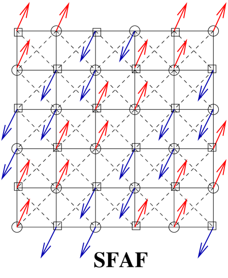
Figure 1: (Color online) The superferro-antiferromagnetic (SFAF) or $4\times 4$ ground state of the nn and nnn Ising model for $-|J_{2}|<J_{1}<|J_{2}|$.

Phase Diagram

The phase diagram for the model was introduced in Ref. Chitov and Gros, 2005 for varying parameters $J_{1}$, $J_{2}^{a}$ and $J_{2}^{b}$. The result is a three-dimensional qualitative phase diagram including ferromagnetic and various antiferromagnetic phases (Fig. 2 of Ref. Chitov and Gros, 2005). In the present work the focus lies on a one-dimensional cut through this phase diagram with a varying nn coupling $J_{1}$ and a fixed value $J_{2}^{a}=-J_{2}^{b}$. The finite-temperature phase diagram $T_{c}(J_{1}/|J_{2}|)$ was qualitatively sketched in Fig. 6 of Ref. Chitov and Gros, 2005. Here we present a quantitative diagram in Fig. 2, obtained by the direct MC simulations along with analytical work. Note that the transition temperatures are invariant under the change of the sign $J_{1}\rightarrow-J_{1}$; this was double-checked in particular for $|J_{1}|<|J_{2}|$. For the interactions $|J_{1}|>|J_{2}|$ the numerical critical temperatures were determined using the Binder cumulants for different lattice sizes.Binder (1981a, b) From the intersection point of these cumulants the critical point can be estimated.Landau and Binder (2000); Kalz et al. (2008)

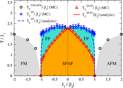
Figure 2: (Color online) Phase diagram of the anisotropic Ising model for varying nn interactions $J_{1}/|J_{2}|$. Three different ground state configurations: Néel order (AFM) for $J_{1}>|J_{2}|$, superferro-antiferromagnetic order (SFAF) for $-|J_{2}|<J_{1}<|J_{2}|$ and ferromagnetic order (FM) for $J_{1}<-|J_{2}|$ are separated by the quantum critical points at $J_{1}=\pm|J_{2}|$. The three phases (disordered, floating, and $4\times 4$) meet at the (exactly solvable) Lifshitz point at $J_{1}=0$. Critical temperatures are determined using Binder cumulants for $|J_{1}|>|J_{2}|$ (energy scale is set to $|J_{1}|$ here) and estimated from energies, specific heats and order-parameter behavior for $|J_{1}|<|J_{2}|$ (energy scale is set to $|J_{2}|$). The transition temperatures in this regime strongly depend on the system size – here $L\leq 200$ (see text for more details). The red solid line for $T_{c}^{SFAF}$ is obtained from Eq. (10). The dashed blue line for $T_{c}^{FP}$ is given by the low-temperature Eq. (6) and Eq. (11) at $0.782(5)\lesssim J_{1}/|J_{2}|\leq 1$ and connects $T_{c}^{FP}$ at $J_{1}/|J_{2}|\approx 0.782(5)$ with the Lifshitz point as a guide to the eye. Note also the agreement with a qualitative sketch in Ref. Chitov and Gros, 2005.

On the other hand for $|J_{1}|<|J_{2}|$, the extraction of critical temperatures is more complicated since the order parameter for the $4\times 4$ state and its Binder cumulant show a strong finite-size dependence. Thus, for the estimation of the critical temperatures in Fig. 2 energies and specific heats were also taken into account.

The nature of the phase transitions for $J_{1}>|J_{2}|$ and $J_{1}<-|J_{2}|$ is of second order and belongs to the Ising universality class. However, according to the prediction of Ref. Chitov and Gros, 2005, the transition from the high-temperature paramagnetic phase to the SFAF state is not direct but rather involves an intermediate floating phase which will be the main topic of the following sections.

III Monte-Carlo and Analytical Results

The MC simulations allow to calculate the energy, specific heat and various order parameters for a wide temperature range and different parameters $J_{1}$ for finite lattice systems. Especially the analysis of the finite-size behavior and the extraction of the values for the thermodynamic limit is crucial in the investigation of incommensurate phases.

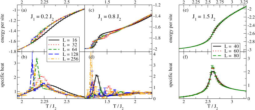
Figure 3: (Color online) Energies and specific heats for some values of nn coupling $J_{1}>0$. In Figs. (a) and (c) multiple steps appear which differ for different system sizes before reaching the ground-state energy $E_{\text{SFAF}}=-2\,|J_{2}|$. As a comparison a converged energy development for the phase transition to the AFM state is shown in (e) – $E_{\text{AFM}}=-2\,J_{1}$. The specific heats in (b) and (d) show multiple peaks which coincide with the steps in the energies shown above whereas in (f) only a single peak is observed which converges at the single transition temperature $T_{\text{c,AFM}}$.

For the simulations we used a Metropolis-single-spin updateMetropolis et al. (1953) with an additional exchange MC step.Hukushima and Nemoto (1996); Hansmann (1997); Katzgraber et al. (2006) As a starting configuration for several independent runs we selected the $4\times 4$ state in the appropriate parameter region for all temperatures and performed $10^{6}$ thermalization steps. This choice was reasoned in the large energy steps between different states in the incommensurate region (see below) and already proved itself very successful in a similar work on a frustrated Ising model.Rastelli et al. (2010)

III.1 Energy and Specific Heat

The behavior of the energy already indicates that the ordering processes for the two phase transitions – to the AFM/FM phase and to the $4\times 4$ state – differ significantly. In Fig. 3 the temperature dependence of the energy and specific heat is shown for three cases: For $J_{1}=0.2\,|J_{2}|,\,0.8\,|J_{2}|$ transitions to the $4\times 4$ state are compared with an Ising-phase transition at $J_{1}=1.5\,|J_{2}|$.

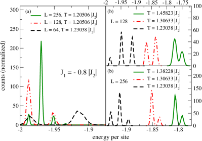
Figure 4: (Color online) Energy histograms for some transitions at $J_{1}=0.8\,|J_{2}|$: Double-peak features are very prominent for the ground-state transition (a) and intermediate transitions at $L=128$ (b) and at $L=256$ (c) as well. However, the energy gaps are not stable and seem to vanish for all histograms in the thermodynamic limit. Note also the different energy scales in panels (b) and (c).

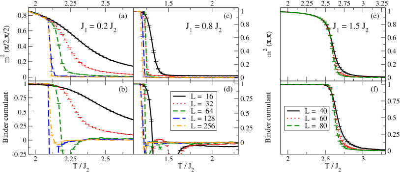
Figure 5: (Color online) Order parameters and Binder cumulants for the $4\times 4$ phase, i.e., moments of the structure factor $S(\pi/2,\pi/2)$ for the same parameters as in Fig. 3. Although in panels (a)-(d) a strong finite-size dependence is visible the convergence of the observables is evident. However, an extraction of the exact transition temperature to the ground state from the intersection of the different Binder cumulants is only possible for the AFM case in panel (f).

The multiple steps in the energies (Figs. 3(a) and (c)), which in addition are shifted for different system sizes $L$, hint towards an unusual ordering in the model that involves different size-dependent intermediate states. This strong size dependence suggests already incommensurate ordering.

Even more prominent than the steps in the energy are the peaks in the corresponding specific heat (Figs. 3(b) and (d)). They coincide with the steps in the energy and prove the existence of several intermediate states. The number of these states obviously depends on the system size; in particular in Fig. 3(d) for each system size ($L=16,\,32,\,64,\,128$) more peaks are distinguishable. However, another feature is observed: The position of the last peak, i.e., for the lowest temperature ($T\approx 1.23\,|J_{2}|$), converges with increasing system size. A comparison with the energy curve above (Fig. 3(b)) shows that below this temperature the system is ordered in the $4\times 4$ state according to the energy value. Thus the final transition to the ground state is locked at a finite temperature similarly to the conventional transitions into the AFM or FM states (compare, e.g., Fig. 3(f)).

For a first characterization of the variety of transitions we recorded energy histograms. In Fig. 4 we show energy distributions at $J_{1}=0.8\,|J_{2}|$ for system sizes $L=64$, $L=128$ and $L=256$ at different temperatures. As expected by the stepwise behavior of the energy, the histograms show double peaks for selected temperatures (at the size-dependent transitions temperatures between intermediate states and to the ground state). The position of the ground-state transition is locked for the three histograms shown in Fig. 4(a) but the peak-to-peak distance varies drastically with the systems size: Essentially the gap between the prominent peaks in the energy distribution shrinks by a factor two while the linear system size is doubled. The same behavior can be extracted for the intermediate transitions. In Figs. 4(b) and (c) histograms are shown which are recorded at higher temperatures for (b) $L=128$ and (c) $L=256$. The multiple-peaked features are again very prominent but the peak-to-peak distances shrink (note the different energy scales for both figures) and the temperatures are shifted as well.

Thus, according to the analysis of energy distributions all finite-size transitions show strong first-order behavior.Berg (2004) However, this seems not to hold in the thermodynamic limit since the energy gaps tend towards zero. Similar behaviour was observed in the 2D ANNNI modelRastelli et al. (2010) and for the isotropic version of the present model.Kalz and Honecker (2012)

III.2 Order Parameters and Correlation Functions

To gain further insight into the ordering process of the system it is useful to define order parameters and analyze their behavior around the phase transitions. The order parameters for the FM and AFM phases are readily defined as magnetization and staggered magnetization which can also be expressed via the spin-structure factors

$$S(\mathbf{q})=\sum_{i,j}e^{i\mathbf{q}(\mathbf{r}_{i}-\mathbf{r}_{j})}S_{i}S_{j}$$ (2)

with ordering wave vectors $\mathbf{q}_{\text{FM}}=(0,0)$ and $\mathbf{q}_{\text{AFM}}=(\pi,\pi)$. The wave vector for the SFAF phase is given by $\mathbf{q}_{44}=(\pi/2,\pi/2)$; the (square) unit cell has four lattice spacings in each direction (see Fig. 1). The square root of the normalized structure factor at this wave vector yields a good order parameter. The calculation of this order parameter can be implemented also using a staggered magnetization

$$m_{4\times 4,k}= \sqrt{\frac{S(\pi/2,\pi/2)}{N}}=\frac{1}{N}\sum_{i}(-1)^{f_{k}(r_{i}^{x},r_{i}^{y})}S_{i}$$ (3)

$$f_{0}(r^{x},r^{y})=[(r^{x}+r^{y})/2]\%\,2$$

$$\wedge~{} f_{1}(r^{x},r^{y})=[(r^{x}+r^{y}+1)/2]\%\,2\,.$$ (4)

The modulo operation ’$\%\,2$’ yields values zero and one, and the two versions $f_{0,1}$ account for the degeneracy of the ground state, i.e., a shift of all spins by one lattice spacing. In addition both states can be flipped completely. In Fig. 5 this order parameter and its Binder cumulantBinder (1981a, b)

$$U_{B}=\frac{3}{2}\left(1-\frac{\langle m^{4}\rangle}{3\langle m^{2}\rangle^{2}}\right)$$ (5)

are shown for increasing lattice sizes and nn couplings $J_{1}=0.2\,|J_{2}|$ (panels a, b) and $J_{1}=0.8\,|J_{2}|$ (panels c, d). As a comparison in panels (e, f) we show the behavior of the AFM order parameter and its Binder cumulant; from the intersection point the transition temperature can be extracted. However, for $|J_{1}|<|J_{2}|$, i.e., for the transitions to the $4\times 4$ state such an analysis is hampered by strong finite-site effects which cause an unusual behavior at the transition: The cumulants do not intersect in a single point and exhibit several dips for intermediate temperatures. To properly understand the numerical results we must recall that the paramagnetic and the $4\times 4$ phases are separated by the intermediate floating phaseChitov and Gros (2005) which, in particular, does not have a conventional local order parameter.

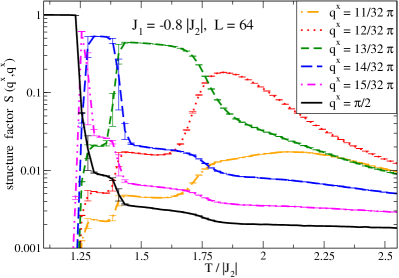
Figure 6: (Color online) Structure factors $S(q^{x},q^{x})$ for a series of momenta $0<q^{x}\leq\pi/2$ vs. temperature. The transitions between the intermediate states are clearly visible. Note also the stepwise behavior of the signals which is only recognizable in the logarithmic scale.

III.3 Floating Phase (analytical)

The key to the analytical treatment of the floating phase comes from the observation that the $4\times 4$ phase in the ground state has exactly the same pattern (2 rows of “up" spins, then 2 rows of “down" spins, or ($++--$) for brevity) as the antiphase of the 2D ANNNI model (cf. Fig. 1) when viewed along the ferromagnetic diagonals. So the Villain-Bak theory,Villain and Bak (1981) developed for that model, can be adapted here with minor modifications. In the vicinity of the QCP ($J_{1}=|J_{2}|$) at low temperature our model can be mapped onto an effective free-fermionic model which accounts for the dynamics of the domain walls. In the floating phase these walls are not straight anymore. The number density of domain walls $\kappa$ is determined via minimization from the following equation valid at low temperature:

$$s(\kappa)=-2\beta(J_{2}-J_{1})\exp(2\beta J_{2})~{},$$ (6)

where

$$s(\kappa)\equiv\frac{1}{1-\kappa}\cos\frac{\pi\kappa}{1-\kappa}-\frac{1}{\pi}\sin\frac{\pi\kappa}{1-\kappa}~{},$$ (7)

and from the physical meaning of $\kappa$, it is bound $0<\kappa<1/2$. The correlation function in the direction perpendicular to ferromagnetic diagonals decays algebraically in the floating phase

$$\langle S(\mathbf{r}^{\prime}+\mathbf{r})S(\mathbf{r}^{\prime})\rangle\sim r^{-\eta}\cos(\mathbf{q}\cdot\mathbf{r})$$ (8)

with the power-law index

$$\eta=\frac{1}{2}(1-\kappa)^{2}~{},$$ (9)

and the wave vector of oscillations $q=\pi\kappa$ determined by the density of walls $\kappa$. This floating phase is bound by the low-temperature SFAF phase and the disordered (paramagnetic) phase at higher temperatures. The critical temperature of the phase transition from the floating into the $4\times 4$ phase is given by the Müller-Hartmann–Zittartz method in the framework of the free fermionic approximation:Villain and Bak (1981); Müller-Hartmann and Zittartz (1977)

$$\sinh 2\beta J_{2}\cdot\sinh 2\beta(J_{2}-J_{1})=1~{},$$ (10)

written here for $J_{1},J_{2}>0$. As one can see from Fig. 2, this equation agrees nicely with the numerical MC results, reproducing even the exactly known Ising value of $T_{c}$ at $J_{1}=0$ (the Lifshitz critical point). Qualitatively, the phase transition from the floating into the $4\times 4$ phase can be understood as freezing of the domain walls into the ($++--$) structure.

On the other part of the diagram, with the increase of temperature the floating phase becomes unstable and undergoes a phase transition into the disordered phase when the dislocations start to proliferate in the network of the domain walls. In this sense the phase transition from the (gapless) floating to the (gapped) disordered phase is topological, not accompanied by the appearance/disappearance of any local order parameter. It is analogous to the vortex unbinding transition in the classical 2D XY model, and the results within the approach due to Villain and Bak can be traced to their counterparts in the Kosterlitz-Thouless theory. The floating phase becomes unstable at the critical value of the walls density $\kappa_{c}$ (or at the wave vector $q_{c}=\pi\kappa_{c}$). It is determined from the following ansatz:

$$\kappa=1-\frac{1}{\sqrt{2}[1+\exp(-4\beta J_{1})]^{1/2}}~{}.$$ (11)

The critical temperature $T_{c}$ and density $\kappa_{c}$ are found from solution of the system of equations (6) and (11). The result of the numerical solution of these equations for $\kappa_{c}$ (and thus for the critical wave vector $q_{c}=\pi\kappa_{c})$ is given in Fig. 7.

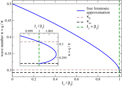
Figure 7: (Color online) The critical domain wall density $\kappa_{c}=q_{c}/\pi$ ($q_{c}$ is the critical ordering wave vector) as a function of couplings. For each given coupling ratio the wave vector grows from $q=q_{c}$ at the critical temperature of the transition from the disordered to the floating phase $T_{c}^{FP}$ up to $q=\pi/2$ at the critical temperature $T_{c}^{SFAF}$ of the transition to the $4\times 4$ phase. The lower bound of $\kappa$, $\kappa_{m}=1-1/\sqrt{2}=0.2929$ and the reentrance boundary (see the text) $\kappa_{0}=0.3008$ are also shown.

$T_{c}^{FP}$ of the transition from the floating to the disordered phase is shown in Fig. 2 by a dashed blue line. The low-temperature equation (6) does not work well at $J\ll|J_{2}|$, since the curve for $T_{c}$ “overshoots" the exactly solvable Lifshitz point $J_{1}=0$. Contrary to Eq. (10), Eq. (6) does not cross over smoothly to the exact result at $J_{1}=0$ (note that $s(1/2)=-2$). This indicates the need for a better theory, taking into account, e.g., fermionic interactions at arbitrary temperature, which we relegate for future work.

In the vicinity of the QCP the system of equations (6) and (11) can be solved analytically. An interesting feature of the equations is a small reentrance effect, when the floating phase enters slightly into the FM and AFM domains $|J_{1}|>|J_{2}|$. The reentrance boundary is given by $\kappa_{c}=\kappa_{0}$, where $\kappa_{0}\approx 0.3008$ is the root of $s(\kappa_{0})=0$. The critical temperature at the point of reentrance can be evaluated as:

$$\frac{T_{c}}{J_{2}}\bigg{|}_{|J_{1}|=|J_{2}|}\approx-4/\ln\big{(}2^{\frac{3}{2}}(\kappa_{0}-\kappa_{m})\big{)}\approx 1.05~{},$$ (12)

where $\kappa_{m}=1-1/\sqrt{2}=0.2929$ is the lower bound of $\kappa$. The bound follows from the stability condition for the floating (Kosterlitz-Thouless) phase:

$$\eta<1/4~{}~{}\Longleftrightarrow~{}~{}\kappa>\kappa_{m}$$ (13)

One can also find that the critical temperature vanishes at the QCP as:

$$\frac{T_{c}}{J_{2}}\approx 2/\ln\Big{(}\frac{A}{|J_{1}/J_{2}|-1}\Big{)}~{},$$ (14)

where

$$A\equiv\frac{1}{2}s^{\prime}(\kappa_{0})(\kappa_{0}-\kappa_{m})\approx 0.04~{}.$$ (15)

At the QCP $\kappa\to\kappa_{m}$ and the correlation function index tends to the free fermionic (Ising) value $\eta\to 1/4$, while in the whole region of the floating phase $1/8\leq\eta\leq 1/4$. The effect of reentrance does not contradict the earlier predictionChitov and Gros (2005) that the floating phase can be adjacent only to the SFAF phase (commensurability parameter $p=4$) of the present nn and nnn Ising model, since there are no commensurate-incommensurate transitions with small $p^{2}<8$, because then $\eta=2/p^{2}$ would violate the condition (13).Bak (1982); Selke (1988); Liebmann (1986) Numerically, the reentrance is very small, and the reentrant regions do not overlap with the FM or AMF phases. It could well be an artefact of the low-temperature approximation (6), however, for a reliable test by MC simulations parameter region is too small.

III.4 Floating Phase (Monte-Carlo)

To verify the predictions for the floating phase, we calculated the structure factors for symmetric momenta on the line $\mathbf{q}_{\text{FM}}=(0,0)\rightarrow\mathbf{q}_{44}\rightarrow\mathbf{q}_{\text{AFM}}=(\pi,\pi)$. We observed finite signals for some structure factors depending on the sign and value of $J_{1}$ and more important also depending on the lattice size. Exemplary we show several structure factors at $J_{1}=-0.8\,|J_{2}|$ in Fig. 6 in a logarithmic scale for a broad temperature range. Due to the computational effort here only $L=64$ is chosen, but nevertheless a cascade of signals can be seen which starts at a critical momentum $q_{c}^{x}<\pi/2$ and ends up in the ground-state order parameter with $q_{44}^{x}=\pi/2$. As we show above, the Villain-Bak theory for this model predicts that the intermediate floating phase is characterized by a single wave vector $\mathbf{q}$ while in the MC results for all momenta

$$\mathbf{q}_{\text{inc.}} =(q^{x}_{\text{inc.}},q^{x}_{\text{inc.}})\quad$$

$$\text{and}\quad\begin{cases}q^{x}_{c}\leq q^{x}_{\text{inc.}}<\pi/2&\text{for }J_{1}<0\\ \pi/2<q^{x}_{\text{inc.}}\leq q^{x}_{c}&\text{for }J_{1}>0\end{cases}\,.$$ (16)

a non-zero contribution can be observed. The left-hand side of Fig. 9 shows the structure factors for several $\mathbf{q}$’s also in a color-coded plot for $L=32$ at $J_{1}=-0.5|J_{2}|$ (upper left panel) and $L=64$ at $J_{1}=+0.8|J_{2}|$ (lower left panel). The behavior described in Eqn. (16) can be seen very nicely in these plots. In conclusion in the intermediate phase the structure factor shows finite signals for certain momenta which depend (i) on the sign and magnitude of the nn interaction and (ii) on the lattice size. This can be explained by the simple fact that for a discrete lattice the number of moments $q_{\text{inc.}}$ between $q_{c}(J_{1})$ and $q_{44}=\pi/2$ increases with the system size.

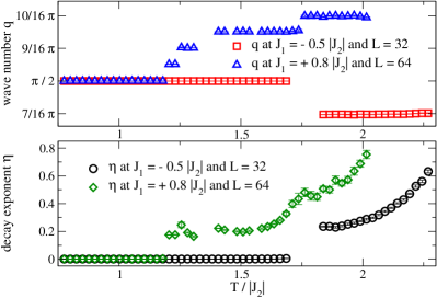
Figure 8: (Color online) Results for the fit parameters of Eqn. 8 when applied to the finite systems for $L=32$ at $J_{1}=-0.5\,|J_{2}|$ and for $L=64$ at $J_{1}=+0.8\,|J_{2}|$. In the upper panel the development of the wave number is shown which reflects the behavior of the structure factors given in the left-hand side of Fig. 9. In the lower panel the algebraic decay exponent is shown: For the intermediate phase a saturation at different levels can be observed before it holds $\eta=0$ in the ground state. (Values in the vicinity of transitions are left out since there the fitting fails.)

Furthermore in Fig. 6, the stepwise behavior of the structure factor at the transitions between different momenta is very prominent. However, this feature is also due to the discrete spectrum of the momenta on a finite lattice. As already observed in the energy histogram finite-size effects play a crucial role in the intermediate phase. In the thermodynamic limit the temperature dependent momentum $\mathbf{q}(T)$ locks smoothly into the ground-state value $\mathbf{q}_{44}$.

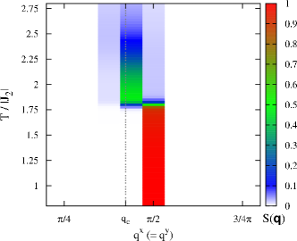
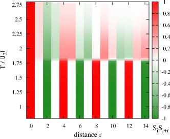
(a) $L=32$; $J_{1}=-0.5\,|J_{2}|$

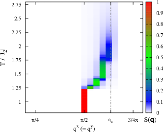
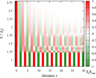
(b) $L=64$; $J_{1}=+0.8\,|J_{2}|$

Figure 9: (Color online) Structure factors (left) and correlation functions (right) calculated from two different systems shown in color code. The stepwise behavior of the structure factors coincides with the distinguished temperature regions in the correlation functions, and the features clearly depend on $J_{1}$ and $L$. The critical momentum $q_{c}$ is determined numerically as described above and shown in Fig. 7.

The size dependence of the signals in the structure factors show already strong indications for unconventional ordering in the system before the actual ground state is reached. A further analysis relies on the evaluation of correlation functions. On the right-hand side of Fig. 9 we present correlation functions calculated in one row or column of the lattice for $L=32$ at $J_{1}=-0.5|J_{2}|$ (upper right panel) and $L=64$ at $J_{1}=+0.8|J_{2}|$ (lower right panel). These correlation functions clearly show non-fitting oscillatory behavior in the region of higher temperatures before the system orders in the ground state with its four-site period. An analysis of these oscillations by fitting Eqn. (8) at each temperature step yields a good agreement in a wide temperature range. The resulting decay exponent $\eta$ and the wave number $q$ can be extracted. Since the correlations are calculated in one dimension only, the wave vector is reduced to one component here. Furthermore, this wave number obviously coincides with the symmetric entries of the wave vector of the corresponding structure factor which are shown on the left-hand side of Fig. 9. The results for $q$ (upper panel) and $\eta$ (lower panel) are given in Fig. 8.

In the plot fitting parameters in the vicinity of transitions and for high temperatures are left out since at these points the fit fails and does not yield meaningful results. The upper panel (wave numbers) only reproduces the results from the structure factors but the lower panels shows that in the intermediate phase the behavior of a floating phase is recovered. The fits of the decay exponent give reasonable (taking into account the strong finite size effects) results in the floating phase. At low temperatures the exponent saturates at $\eta\sim 0.2$, while below $T_{c}$ into the $4\times 4$ phase with the long-range order parameter it adopts the value $\eta=0$.

IV Conclusion

An anisotropic version of the frustrated $J_{1}$-$J_{2}$ Ising model was investigated using mainly MC simulations, supplemented by analytical treatments. In particular the phase transition into an antiferromagnetic ground state constituted of two sublattices in collinear order ($4\times 4$ phase) was analyzed. It was predicted earlier by Chitov and GrosChitov and Gros (2005) along with an unconventional floating phase which appears for intermediate temperatures before the ground state is reached. For analysis of the floating phase the Villain-Bak theoryVillain and Bak (1981); Bak (1982) with some small modifications was utilized for the present model. In the floating phase the theory predicts no local order parameter, algebraically decaying correlation functions with the power-law exponent $\eta$, modulated by a plane wave with a (single) incommensurate wave vector $q$ depending on couplings and temperature. The theory also allows to quantitatively describe the smooth evolution of the wave vector from its critical value $q_{c}$ at the critical temperature between the disordered and floating phases towards its commensurate value at the boundary of the $4\times 4$ phase. The critical temperatures between these phases are also evaluated. Qualitatively, the theory gives the picture of the transition from the floating to disordered phase via proliferation of dislocations of the domain walls, which is analogous to the Kosterlitz-Thouless transition of vortices in the classical XY model, while the transition into the commensurate phase occurs via freezing of the domain walls into the $4\times 4$ structure.

The nature of the intermediate phase was also analyzed using correlation functions and the corresponding structure factors in the MC simulations. It appears in the simulations of the finite-size system that the phase is not described by a single wave vector but rather a set of neighboring wave vectors. The transitions in finite lattices between states with different momenta are sharp, however, in the thermodynamic limit energy gaps seem to vanish. Thus the phase is best described by a temperature dependent wave vector whose discrete spectrum is smeared out in the thermodynamic limit. The momentum varies from a starting vector $\mathbf{q}_{c}(J_{1}/|J_{2}|)$ and locks smoothly into $(\pi/2,\pi/2)$. The nature of this phase was further analyzed by fitting the correlation functions by a combination of algebraic decay and oscillatory behavior. The agreement in the intermediate phase is very good and we conclude from this result that the state is best described by a floating phase consistently with the analytical predictions. The model’s phase diagram in Fig. 2 summarizes most of our MC and analytical results.

As for the further work, we expect a very interesting behavior of the present model when the transverse field is included, especially near quantum criticality.Chitov and Gros (2005) Another interesting direction is the 3D generalization of the model, where the devil’s staircase, similar to the one in the 3D ANNNI model,Selke (1988); Bak (1982) is expected.Chitov and Gros (2004b) It appears that the devil’s staricase in the 3D extension of the present model was already observed experimentally.Ohwada et al. (2001)