The role of convective structures in the poloidal and toroidal rotation in tokamak

Abstract

The connection between the poloidal and the toroidal rotation of plasma in tokamak is important for the high confinement regimes, in particular in reactor regime. The sudden onset of closed convection structures in the poloidal section, due to the baroclinic production of vorticity, will sustain a fast increase of the poloidal velocity and a substantial effect on the toroidal rotation. However this is limited to the short time of the onset transition. In real plasma however there is random generation and suppression of convection cells and the sequence of these transient events can prove able to sustain the effect on the toroidal rotation. We formulate a simplified model which consists of a laminar sheared, regular, flow situated at the boundary of a region of drift-wave turbulence. Vortical structures, randomly generated in this turbulent region are spontaneously advected toward the flow and are absorbed there, sustaining with their vortical content, the sheared flow. We examine this dynamics in the wavenumber $\mathbf{k}$ space, using reasonable approximations. We derive a system of equations (which is a class of Devay-Stewartson system) and find that indeed, the vortices advected and absorbed into the layer can preserve its regular, poloidal, flow.

1 Introduction

Mixed regimes consisting of large scale flows (H-mode, Internal Transport Barriers) and turbulence are expected to be the current state in ITER. The rotation, either spontaneous or induced, will play a major role in the quality of the confinment. The efficiency of the sheared poloidal rotation to control the instabilities is considerably higher than that of the toroidal rotation but it is usually assumed that the poloidal rotation should be at the neoclassical level due to the damping induced by magnetic pumping. This is true if the drive of the poloidal rotation (besides the neoclassical one) relies on the Reynolds stress produced by a poloidally -symmetric turbulence. Much higher drive of the poloidal rotation is however provided by flows associated with the convective structures that can be generated in the plasma cross-section beyond a threshold in the plasma pressure gradient. This drive overcomes the damping due to the magnetic pumping and the poloidal rotation is sustained. Cells of convection consisting of closed, large scale flows with unique sense of rotation can be spontaneously generated, triggered by streamers sustained by the baroclinic term able to generate vorticity. Similar to the Reyleigh-Benard first bifurcation (from purely conductive to convective regime), the onset is very fast and the drive exerted on the poloidal rotation leads to a fast time variation of the polarization radial electric field. This is sufficient to create a distinction between the phases (first half, second half) of bounce on a banana of trapped ions and, implicitely, leads to acceleration in the toroidal direction. This phenomenological model has been proposed recently [1] and the estimations are compatible with the observed effect of reversal of the toroidal rotation in tokamak. There are several aspects that still must be investigated and in particular the nature of sudden-impulse of the generation of the poloidal flow as envelope of the peripheral velocity of the convective structures. It is only on a very short time interval (onset of convection) that the time variation of the radial electric field can produce a toroidal effect on the bananas. If the convection cells become saturated and stationary then the efficiency of sustaining toroidal acceleration of bananas decreases rapidly to zero. The process must be repeated if it is to sustain its effect on the toroidal rotation.

On the other hand, it is highly improbable that the structure consisting of cells of convection breaking the azimuthal symmetry can exist as a stationary state. This is because the convection in the cells is much more efficient as radial transport of energy than any diffusive process sustained by small scale turbulence and the equilibrium profiles would be modified, suppressing the origin of convection. It is more realistic to regard the generation of convective structures as a stochastic process consisting of a random sequence of transient events, taking place on a range of spatial scales between $\rho_{s}$-scale drift vortices up to cells of convection with dimensions comparable with the minor radius $a$. We should study the way these transitory structures create the impulsive increase of the poloidal velocity such as, on the average, to sustain the toroidal effect on bananas. A marginal stability regime can be established, where the external sources sustain the gradient of the pressure, the convection rolls are formed transitorily and the excess of the gradients relative to a threshold is transformed into pulses of heat and momentum in the radial direction. This problem requires a treatment based on the stochastic nature of the generation and destruction of the transversal convection cells, seen as a random transitory process. Such a treatment simply does not exist, not even for the famous Rayleigh-Benard system.

This problem is important per se, beyond the phenomenological model for the reversal of the toroidal rotation. This process has been identified in experiments on a linear machine [2] and explained in the context of residual stress able to sustain the coherent flow. The sequence consisting of tilt, stretch and absorbtion of drift turbulent eddies was found to contribute significantly to the Reynolds stress. Coalescence of strongly tilted, almost poloidally oriented, eddies and formation of radially periodic and poloidally closed ($m=0$) flow was proposed in [3] as transition to rotation given by the stable solution of the nonlinear equation for the electrostatic potential at the edge (the Flierl-Petviashvili equation). The absorbtion of a coherent convection cell inside a layer of sheared rotation is mentioned by Drake et al. [4]. It has also been discussed in similar terms in Refs.[5], [6].

The structure of the paper is as follows. We formulate a model which is relevant for the physical problem of sustainement of poloidal rotation by stochastic rise and decay of vortices on different scales. We estimate the average density of high amplitude vortices that are generated inside a volume of plasma (in our case it is question of an area within the poloidal cross-section since the third - toroidal - axis is considered irrelevant). Then we remind the known mechanisms on motion of a vortex on a background of gradient of vorticity, in order to see how random elements of vorticity of only one sign will join the  flow layer where they are absorbed. Finally, we examine this dynamics in the wavenumber space $\mathbf{k}$ and derive a model system of equations reflecting the interaction between the laminar flow and the incoming drops of vorticity. This is actually the Davey Stewartson system and indeed, the class of solutions called “solitoffs” show that the final state exhibits unidirectional (poloidal) alignment of the resulting flow. This confirms that the elements of vorticity coming from the turbulent region into the laminar flow do not perturb but are conforming themselves to the geometry of the flow, i.e. in the poloidal direction.

2 Formulation of the model

The effect of advection of impulse-like convection structures (streamers, transient convection rolls of all sizes from $\sim a$ down to the small $\rho_{s}$ scale of high amplitude robust drift vortices) to the layer of sheared laminar flow and their role in sustaining the laminar flow is a process that has aquired recognition for its importance in creating a coherent flow pattern. In the physics of the atmosphere and in fluid physics this is a well known phenomenon. It has been examined within the model of potential vorticity mixing [7] for the generation of an atmospheric jet, the equivalent of sheared laminar flow. Recent numerical simulation indicate the interesting and unexpected random switching of the flow between the two geometries: laminar flow and respectively a periodic chain of positive and negative vortices [8] which indicates that these two states are indeed neighbor in the functional space of the system’s configurations. The examination of the problem in real space is particularly difficult since it requires to analytically describe unequivocally the emergence of a coherent structure out of turbulence. One of the possiblity would be to derive a time-evolution equation for the effective number of degrees of freedom that are involved in the motion, as it results from a Karhunen - Loewe analysis. Such an approach is under examination but with the reserve that it may not really become a quantitative instrument.

Alternatively we can examine the system in the spectral $\mathbf{k}$ space. The wave kinetic equation is the standard instrument to describe the dynamics of the energy density on elementary spectral intervals (seen as pseudoparticles), induced by nonlinear processes of wave turbulence [9]. We must adapt this approach to our particular problem, inspired by similar adaptations that have been made in several cases in the past. The most common models for dissipative equations of motion are the time-dependent Landau - Ginzburg models. The model function is $\psi$, the order parameter of the superfluid. In the absence of dissipation the general form of the equation is [10]

$$\frac{\partial\psi}{\partial t}=2i\Gamma_{0}\frac{\delta H}{\delta\psi^{\ast}}$$

where $\Gamma_{0}$ is a real constant and the hamiltonian is

$$H\left[\psi\right]\equiv\int d^{d}x\left[\frac{1}{2}\left|\mathbf{\nabla}\psi\right|^{2}+\frac{1}{2}\alpha\left|\psi\right|^{2}+\beta\left|\psi\right|^{4}\right]$$

The total number of particles $N=\int d^{d}x\left|\psi\right|^{2}$ must be constant, as well as the energy $E=H\left[\psi\right]=$const. The time dependent LG, is universal and occurs whenever there is a two-phase system and a possible phase transition between them, with a function $\psi$ representing the order parameter. Of course, such a situation is subiacent to our more general and more complex problem. We take this as a suggestion to simplify our problem and reduce our objectives with the promise that they would become more accessible: we will try to prove that the advection of the transient convection structures to the laminar flow layer will not perturb the geometry of the flow, which remains mainly poloidally oriented. Then the conservation of the vorticity will guarantee that the content of vorticity of the individual structure joining the laminar sheared flow will be absorbed into the new, coalesced, flow and further will be redistributed to become homogeneous along the direction of flow. Or, the vorticity of a laminar flow is simply the derivative of the unidirectional velocity with respect to the transverse coordinate. The increase of the content of vorticity in the region of the laminar flow simply means that the total momentum (in case of a slab geometry) or angular momentum (if the flow is confined in a poloidal layer) is increasing. We then have a drive that may sustain the flow against the magnetic pumping. All this now requires to prove that absorbtion of the transient convection structures preserves the laminar flow and merge their vorticity content into the sheared flow.

In connection with our problem of stochastic stationarity of sustainment of poloidal flow by intermittent rise and decay of convection cells we construct a simple model to be investigated. We consider a layer of laminar sheared rotation where we assume that the instabilities are suppressed (this is an ideal representation of the zonal flow or of the $H$-mode layer). The layer is connex to a region where drift-type turbulence exists. The width of the layer is much smaller than the region of turbulence. In the drift-turbulent region there is stochastic generation of convective motions and of strong vortical structures. The physical effect is different in the two limits: for large convective events there is an effect which we see as a jet-like impulse acting on the laminar layer; for small and robust vortices acceding the sheared flow, the effect consists of a forcing applied to the layers of the flow that have the same direction of flow as the rotation in the vortex while the layers where the two directions are opposite are decelerated. This enhances the local gradient of the velocity (i.e. the shear). Since the decelerated layers are in contact with the bulk, turbulent, plasma, the angular momentum is transferred by viscosity. While the thin laminar layer is accelerated, the large mass of turbulent plasma will only get a low rate of compensating rotation. This ensures the conservation of angular momentum. Although large and small vortices interact in different ways with the sheared flow layer, we will attempt a simplified treatment that retains the common aspects.

The shear rate (first derivative of the velocity of flow with respect to the coordinate transversal to the layer) is assumed non-uniform, which is equivalent to a gradient of vorticity (involving the second order derivative). The vorticity starts from zero at the boundary with the turbulent region and increases with the distance from it. Since the background has a gradient of vorticity a vortex will move in a direction which depends on the sign of its vorticity relative to the one of the background: the clumps (positive sign circulation vortices) are ascending the gradient of vorticity, toward the maximum of vorticity in the rotation layer and the holes (negative sign circulation vortices) are moving toward the minimum of vorticity, equivalently - they are repelled from the sheared layer [11]. In short, vortices of only one sign are joining the layer. The clump vortices will be absorbed by the sheared velocity layer with the transformation of their vorticity content into a local enhancement of the shear of the flow. This is a source of momentum which sustains the sheared flow, in particular sustains the sheared poloidal rotation against the damping due to the magnetic pumping. However it may appear as a spotaneous separation of ordered motion out of turbulence, and would pose a problem of entropy decrease. We have to remember that the vortices and the directed motions belonging to convection events are actually supported, via the baroclinic terms, by the equilibrium gradients (which are externally sustained). Similar physical processes are probably behind the formation of the Internal Transport Barriers and the formation of the $H$-mode rotation layer. A last comment is in order, in connection with what appears to be a spontaneous separation of the vorticities of the opposite signs. This is indeed what happens in the $2D$ ideal fluid at relaxation as result of the inverse cascade, and is shown by experiments and numerical simulation [12] and also derived analytically [13]. Similar separation of the two signs of vorticity has been seen for plasma [14] and atmosphere, also supported by analytical derivation [15]. The result is a final state consisting of a pair of vortices of opposite signs that have collected all positive and respectively all negative vorticities in the field (a dipole). We now note that the dipolar state can be realized as either two distinct vortices of opposite signs, or, in a circular geometry, as a central part with vorticity of one sign surrounded by an annular region of vorticity of the opposite sign. Transitions are possible between the two ”dipolar” geometries of vorticity separation and the change is very fast. We only mention this facts in support of our phenomenological representation of the sustainment of the sheared rotation, but we will not develop this subject here.

We take the layer of plasma flow in the $y$ ($\equiv$ longitudinal, streamwise, poloidal in tokamak) direction with sheared velocity varying in the $x$ ($\equiv$ transversal on the layer of flow, radial in tokamak) direction. It is described by a scalar function $\widehat{A}\left(x,y,t\right)$ which is the complex amplitude of slow spatial variation of the envelope of the eddies of drift turbulence. From $\widehat{A}\left(x,y,t\right)$ the components of the velocity are derived as $\mathbf{v}_{E}=-\mathbf{\nabla}\widehat{A}\left(x,y\right)\times\widehat{\mathbf{n}}/B$ where $\widehat{\mathbf{n}}$ is the versor of the magnetic field. We also define a scalar function $\phi\left(x,y,t\right)$ which represents the field associated to the incoming vortices that will interact and will be absorbed into the sheared, laminar, flow, transfering to it their vorticity content. The process in which a localized vortex is peeled-off and absorbed into the sheared flow may be seen as a transfer of energy in the spectrum from the small spatial scales involved in the structure of the vortex toward larger spatial scales of the sheared flow, with much weaker variations on the poloidal direction. This can be seen as a propagation in $\mathbf{k}$ space.

We must first estimate what is the number of high amplitude, robust vortices that are generated by the drift-turbulence in a unit area. This problem is treated in the Appendix 1 where it is shown that the density of strong vortices is $n=3/\left(\pi\lambda^{2}\right)$ where $\lambda$ is the typical size of the drift eddies normalized to $\rho_{s}$.

3 How these vortices ascend to the flow layer?

The answer is: due to the existence of the background gradient of vorticity. This has been clearly described for non-neutral plasma in [11] and is also known in the physics of fluids [17], the physics of the atmosphere [16] and in astrophysics (accretion disks) [18].

Since the background has a gradient of vorticity a vortex will move in a direction which depends on the sign of its vorticity relative to the one of the background:

• the prograde vortices are moving toward the maximum of vorticity and

• the retrograde vortices are moving toward the minimum of vorticity.

The prograde vortices eventually are absorbed by the sheared layer and they contribute with their vorticity content to the momentum of the background flow. This is a source of momentum which sustains the sheared flow, in particular sustains the sheared poloidal rotation against the damping due to the magnetic pumping.

A clump of vorticity (positive circulation $\Gamma_{v}>0$) goes up the gradient of background vorticity. For a sheared velocity flow with poloidal velocity $v_{\theta}$ increasing linearly with radius, with a coefficient $Q$

$$v_{\theta}=Qr$$

but in a layer which has background vorticity $\zeta_{0}^{\prime}\ \$along$\ \ r$ , the radial motion of the positive vortex (position $r_{v}$) is

$$\frac{dr_{v}}{dt}=\zeta_{0}^{\prime}l^{2}\ln\left(\frac{cr_{v}}{l}\right)\arctan\left(\left|Q\right|t\right)$$

where $l\equiv\sqrt{\left|\Gamma_{v}/\left(2\pi Q\right)\right|}$ [19]. Schecter and Dubin [11] find $c\lesssim 1$. The position of the vortex is greater but comparable to the typical length $l$, $r_{v}/l\gtrsim 1$. The $\arctan$ function is bounded by $\pi/2$.

The negative-circulation vortices, $\left(\Gamma_{v}<0\right)$ called holes are moving in the opposite direction therefore they remain in the turbulent region and are repelled by the layer of sheared flow with global conservation of angular momentum. This means that only vortices of a certain sign ascend to the flow and are absorbed in it. In the following we will analyse this process as an interaction between the two fields: $\widehat{A}\left(x,y,t\right)$ and the field representing the incoming vortices.

4 Dynamics in the $\mathbf{k}$ - space of the interaction between the laminar flow field and the field of the vortical cells

In order to derive a dynamic equation for the scalar streamfunction of the sheared flow $\widehat{A}\left(x,y,t\right)$ we remind the properties resulting from multiple space-time analysis of a turbulent field, like the drift waves interacting with a coherent, sheared flow. The typical equation in the hydrodynamic description is Rayleigh-Kuo or barotropic equation and the multiple space-time scale analysis leads to the Nonlinear Schrodinger Equation for the amplitude $W\left(x,y,t\right)$ of the envelope of the oscillatory waves excited in the fluid [20]. The general structure of this equation is

$$i\frac{\partial W\left(x,y,t\right)}{\partial t}=\Delta W\left(x,y,t\right)-\gamma\left|W\right|^{2}W^{\ast}$$ (1)

The interesting term is the nonlinearity (the last term) which may be seen as arising from a self-interaction potential $V\left[W\left(x,y,t\right)\right]$ (see the next Section). The later potential results naturally from the multiple scale analysis and it is the effect on the envelope amplitude of the nonlinearity consisting of convection of the vorticity by its own velocity field. We must work with an amplitude $A\left(k_{x},k_{y},t\right)$ in the spectral $\mathbf{k}-$space, which we see as the envelope of oscillations representing propagation of perturbation in the spectrum, this propagation being a reflection of what is the process of the incoming vortex dissolving itself and being absorbed by the flow, - in the physical space. Looking for an analytical model for $A$ in the $\mathbf{k}$-space we will use the structure which is suggested above.

We expect to have a diffusion in $\mathbf{k}-$space and the same self-limitting nonlinear term

$$i\frac{\partial A\left(k_{x},k_{y},t\right)}{\partial t}=\left(\frac{\partial^{2}}{\partial k_{x}^{2}}+\frac{\partial^{2}}{\partial k_{y}^{2}}\right)A\left(k_{x},k_{y},t\right)-\gamma\left|A\right|^{2}A^{\ast}+S$$ (2)

and we have added a source $S$ that represents the interaction of the basic flow $A$ with the vortices that are randomly generated in the drift turbulence and are joining the flow.

The addition of “drops” of vorticity is represented by the $\mathbf{k}$-space scalar function $\phi$

$$\phi\left(k_{x},k_{y},t\right)$$ (3)

Several space scales are present in the structure of the function $\phi\left(x,y,t\right)$ in real space. The reason is that we must consider that the vortices that are continuously generated in the turbulent region have two characteristics:

• the space extension of individual vortices coming into the layer has a wide range of values. The range extends from vortices of the dimension $\rho_{s}$ (the natural result of excitations sustained by the ion-polarization drift nonlinearity) up to convective events representing streamers with -closed (roll-type) geometry and spatial extension given by the inverse of $k_{\theta}=m/r$ for $m$ of only few units.

• the spatial distribution of the place where these vortical structures are reaching the layer of sheared flow is random over practically all the circumference of the poloidal flow.

We will draw conclusions about the $\mathbf{k}$-space profile of $\phi$ based on the contributions coming in from various scales in the real space. The most simple description neglects the random aspect of the content of $\phi$ and simply ennumerates the possible spatial scales. For this we adopt a discrete representation of the dimensions of vortices, starting from a minimal size of the order of $\rho_{s}$ up to a low-$m$ fraction of the circumference $2\pi r$ of the poloidal rotation layer, this last scale corresponding to large convection roll-type events.

The above elementary assumption, i.e. the discrete number of space extension of vortices, implies that the function $\phi\left(k_{x},k_{y}\right)$ presents higher amplitudes around wavenumbers $\mathbf{k}$ which correspond to the inverses of the spatial scales. The simplifying assumption which takes uniform spatial distribution of the events of arrival of vortices (of any scale) to the layer implies periodicities on various spatial scales.

We consider separately the $y$ direction (poloidal). One periodicity can be at the level of a smallest vortex, $k_{y}^{\left(1\right)}$. This means that a sequence of maxima of $\phi\left(x,y\right)$ appear with spatial periodicity $2\pi/k_{y}^{\left(1\right)}$ and this corresponds to the addition of smallest vortices into the flow layer. Further, on a longer space scale there is another periodicity, $k_{y}^{\left(2\right)}$. This means that the sequence on the lower scale (with much denser spatial granulations of vorticity, $2\pi/k_{y}^{\left(1\right)}$) is modulated on a longer space scale with a periodicity $2\pi/k_{y}^{\left(2\right)}$. This is because larger vortices (but not yet convection rolls) are absorbed into the flow layer. Large vortices carry smaller vortices. These considerations can be extended to other, intermediate, levels of periodicity. Finally we can have the largest (accessible) spatial scale $2\pi/k_{y}^{\left(n\right)}$ where a convective event occurs as a result of a stochastic event, or a streamer sustained by the baroclinic term and having the close-up property.

We note that the periodicity in the poloidal direction $y$ cannot occur without a corresponding periodicity in the $x\equiv$ radial direction, as far as the vortices and convective events are concerned. It is reasonable to assume a linear dependence : small scale periodicities in the poloidal direction (small scale robust drift vortices) occur on a similar radial scale, i.e. again small periodicity in the $x\equiv$ radial direction. With larger $y$ wavelengths, we expect to involve also larger radial wavelengths since the physical process involves more fluid motion in the closed-up convection cell.

This suggests a proportionality between the periodicities on the poloidal direction, $y$, and the periodicities on the radial, $x$, direction, in the structure of $\phi\left(k_{x},k_{y}\right)$. This means that the Fourier components along $y$ (e.g. at $k_{y}$) are proportional with the Fourier components along $x$ (at $k_{x}$) with the same proportionality coefficient on all the spectral interval. The fact that there is (assumed) proportionality on the periodicities on $y$ and on $x$, requires for analytical description a hyperbolic operator

$$\left(\frac{\partial^{2}}{\partial k_{x}^{2}}-\frac{1}{a^{2}}\frac{\partial^{2}}{\partial k_{y}^{2}}\right)\phi\left(k_{x},k_{y}\right)\approx 0$$ (4)

where the D ’Alamebrtian operator $\square_{k_{x}k_{y}}\equiv\frac{\partial^{2}}{\partial k_{x}^{2}}-\frac{1}{a^{2}}\frac{\partial^{2}}{\partial k_{y}^{2}}$ is the signature of the correlated periodicities on the poloidal and radial directions of the field $\phi$ representing the incoming drift vortices - up to convection rolls, generated in the drift turbulence region, moving against the gradient of vorticity, and finally absorbed into the rotation layer. The  ”velocity ” $a$ is the ratio of the periods on the two $k$-space directions and we take it $a\approx 1$. The centers of the vortices reach points that belong to the lines $y=\pm ax$. The general form of the solution of the homogeneous equation is

$$\phi\left(k_{x},k_{y}\right)\sim\exp\left(ik_{x}x+ik_{y}y\right)$$ (5)

When $\phi$ is  ”free” it is double periodic and it verifies the above equation. However the destruction (peeling-off) of the incoming vortices and their absorbtion through interaction with the background flow, $A$, is the loss of the double periodicity. The departure relative to the $\mathbf{k}$-space double periodicity (the  ”free” state of $\phi$) feeds the flow field $A\left(k_{x},k_{y},t\right)$ such as to enhance it in spectral regions comparable to those where the vortices are localised, i.e. higher $\left|\mathbf{k}\right|$. Basically, if the free $A\left(k_{x},k_{y},t\right)$ is localised on $k_{y}$ close to $k_{y}\sim 0$ (equivalent to an uniform poloidal flow), the source induced by $\phi$ is a charge which acts through a Poisson equation on the  ”potential” given by the amplitude $AA^{\ast}$. We should recall that we want to represent the physical process in which incoming vortices transfer via absorbtion their vortical content to the sheared flow, sustaining and/or enhancing the poloidal, $y$, rotation. This is mainly manifested as the evolution of an initial oscillation generated by $\phi$ on the $k_{y}$-spectrum with collection of the energy in a region close to $k_{y}\sim 0$, since this corresponds in real space to the uniformization of the flow in the poloidal direction, after an event of absorbtion of a vortex. Then, ignoring the less significant periodicity in $k_{x}$ direction, corresponding to periodic perturbation propagating in the $x$ (radial) direction, the interaction may be represented as

$$-\beta\frac{\partial^{2}}{\partial k_{y}^{2}}\left|A\right|^{2}\approx\left(\frac{\partial^{2}}{\partial k_{x}^{2}}-\frac{\partial^{2}}{\partial k_{y}^{2}}\right)\phi\left(k_{x},k_{y}\right)$$ (6)

The constant $\beta$ is a measure of the permitivity of the equivalent electrostatic problem. Using the specific terminology $\beta$ measures the decrease of the effectiveness of the effect of the charge (right hand side of the Eq.(6)) on the potential $\left|A\right|^{2}$ due to the “polarization”. Essentially, the amount of destruction of the incoming vortex, measured by the departure from the  “free” state by the right hand side of the Eq.(6) is transferred to the background flow by first exciting elementary waves in real space, while $A$ is only an envelope. The perturbation of the sheared flow $A$ (via the left hand side of the Eq.(6)) results from the nonlinear interaction of these excited waves, i.e. by convecting the modified vorticity with the background velocity flow. This is the nonlinear term of the right-hand side of Eq.(2). Then it is reasonable to assume $\beta\approx\gamma$.

Returning to the equation for $A\left(k_{x},k_{y},t\right)$ we specify the interaction between the two fields $A$ and $\phi$ in the simplest way

$$S=2\phi\left(k_{x},k_{y},t\right)A\left(k_{x},k_{y},t\right)$$ (7)

Then

$$i\frac{\partial A\left(k_{x},k_{y},t\right)}{\partial t}=\left(\frac{\partial^{2}}{\partial k_{x}^{2}}+\frac{\partial^{2}}{\partial k_{y}^{2}}\right)A\left(k_{x},k_{y},t\right)-\gamma\left|A\right|A^{\ast}+2\phi A$$ (8)

to which we add the equation for $\phi$,

$$\left(\frac{\partial^{2}}{\partial k_{x}^{2}}-\frac{\partial^{2}}{\partial k_{y}^{2}}\right)\phi\left(k_{x},k_{y},t\right)\approx-\gamma\frac{\partial^{2}}{\partial k_{y}^{2}}\left|A\right|^{2}$$ (9)

These two equations are known as Davey-Stewartson system and our case is DS-I [21]. It is exactly integrable and several analytical solutions are available, in terms of Riemann theta functions or Jacobi elliptic functions. Of particular importance for our physical problem is the long wave limit solutions, as obtained by Chow using the Hirota method. We reproduce here his result [21], with details given in Appendix B.

$$A=\frac{r\left(1-k\right)}{2}\left[\frac{\tanh\left(sk_{x}\right)-\sqrt{k}\mathrm{sn}\left(rk_{y},k\right)}{1+\sqrt{k}\mathrm{sn}\left(rk_{y},k\right)\tanh\left(sk_{x}\right)}\right]\exp\left(-i\Omega t\right)$$ (10)

$$\phi = 2r^{2}\left(1-\frac{E}{K}\right)$$

$$-2r^{2}\frac{k\left(k\mathrm{sn}^{2}\left(rk_{y},k\right)+\tanh^{2}\left(sk_{x}\right)\right)+\left(1+k^{2}\right)\sqrt{k}\mathrm{sn}\left(rk_{y},k\right)\tanh\left(sk_{x}\right)}{\left(1+\sqrt{k}\mathrm{sn}\left(rk_{y},k\right)\tanh\left(sk_{x}\right)\right)^{2}}$$

These solutions are called solitoffs and they decay in all directions except a preferred one. They are  ”semi-infinite solitary waves”. For example, for $k=0.7$ and $r=1$ the solution shows a peak of $\left|A\right|^{2}$ around $k_{y}\approx 0$ which in physical terms means quasi-uniform flow along the poloidal direction. This is compatible with what we expect from this analytical model: the turbulence advects “drops” of vorticity into the rotation layer and this does not destroy the flow but sustains it. It is actually a discrete Reynolds stress, or a process which is reversed version of the usual Kelvin-Helmholtz instability.

5 Discussion

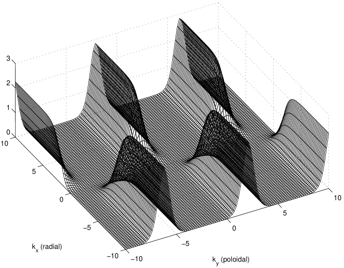
Figure 1: Graphical representation of the solution of the Devay Stewartson system for the parameters $k=0.7$ and $r=1$.

The Figure (1) represents the amplitude of the solution given in Eq.(10). We now want to understand in more detail what was the origin of the final spectral structure (i.e. the solution written above) in our previous analysis, which was mostly qualitative and based on several assumptions.

We note that the solution looks compatible with our idea about the build-up and/or sustainment of a sheared laminar flow out of random convection of momentum from the deep region where turbulence is active. We first refer to the term $-\gamma\left|A\right|^{2}A^{\ast}$. Essentially this term is the quantitative translation of the physical fact that the flow, after a perturbation (which later we will specify as ”absorbing” an incoming vortex), will try to re-establish the uniformity of the flow by spreading the new perturbing vorticity as shear of the flow. Although this is a very approximative image we expect that this term in the action functional (i.e. in the integral of the Lagrangian density) to penalize departures of the flow configurations from uniformity of the flow. The departures are measured as the square of the difference between the actual magnitude of $AA^{\ast}$ and a reference uniform configuration. Then the system moves in the function space in a potential $V\left[\varphi\left(\mathbf{k}\right)\right]$ with two extrema $\pm v$ (symmetric relativ to $\varphi\left(\mathbf{x},t\right)\equiv 0$), so that in its Lagrangian there is a term $\mathcal{L}^{nl}$ of nonlinear self-interaction of the scalar field $\varphi$, of the general type

$$\mathcal{L}^{nl} \sim \int dtd^{2}x\left(\varphi\varphi^{\ast}-v^{2}\right)^{2}$$

$$= \int dtd^{2}x\int dt^{\prime}d^{2}x^{\prime}\left[\varphi\left(\mathbf{x},t\right)\varphi^{\ast}\left(\mathbf{x},t\right)-v^{2}\right]$$

$$\times U\left(\mathbf{x},t;\mathbf{x}^{\prime},t^{\prime}\right)\left[\varphi\left(\mathbf{x}^{\prime},t^{\prime}\right)\varphi^{\ast}\left(\mathbf{x}^{\prime},t^{\prime}\right)-v^{2}\right]$$

with $U\left(\mathbf{x},t;\mathbf{x}^{\prime},t^{\prime}\right)\equiv\delta\left(\mathbf{x}-\mathbf{x}^{\prime},t-t^{\prime}\right)$. This means that the stationary states will try to attain one of the equilbria given by the extremum of $V\left[\varphi\right]$. In our simplified case the ”reference configuration” that the system takes as ground state above which it penalizes any departure is simply $v\equiv 0$. This means that we represent the simultaneous wiping out of the local perturbation and the suppression of the shear, without having any reason for the latter, except for tractability. The potential $\delta\left(\mathbf{x-x}^{\prime},t-t^{\prime}\right)$ makes the uniformity ($v\equiv 0$ in this simplified description) an attractive state, if no source term is present. With $v\equiv 0$ the nonlinearity becomes the same as in the Nonlinear Schrodinger Equation, as we have mentioned above, in the construction of the model.

On the other hand we see that in the presence of a source the solution for fixed, greater than zero, $k_{x}$, is not exactly at the ”poloidal uniform flow” $k_{y}=0$ but shifted, the spectrum is peaked in $k_{y}$ at a small but finite value. This means that our description actually obtains longwave poloidal oscillations but not exactly symmetric $m\equiv 0$ poloidal flow. This shift is due to the average of the spatial extensions of the incoming perturbations and is dependent on the scale factor (’wavelength’) $r$. The two parameters $r$ and $s$ must be seen as representative space scales along the poloidal $\left(y\right)$ respectively radial $\left(x\right)$ directions.

We have simply neglected the structure of the spectrum on $k_{x}$ (radial). In the solution it occurs with a uniform $k_{x}$-space contributions for positive wavenumbers (the $\tanh$ function rises rapidly after a space scale $s$ and remains constant after that for all $k_{x}>1/s$). This means that the structure of the flow on the transversal direction (a cross section along the radius) contains all possible motions and modulations, without however placing emphasis on any of them. It becomes effective the assumption that the convections and vortices are coming in all sizes, and we have neglected the second derivative of the flow amplitude $A$ to $k_{x}$ in Eq.(6), compatible with the approximate independence of $A$ on $k_{x}$.

We note that the identical reproduction of the localized maxium close to $k_{y}\approx 0$ at periodic intervals along $k_{y}$ axis is the result of the periodicity

$$sn\left(rk_{y},k\right)=sn\left(rk_{y}+4K,k\right)$$

of the Jacobi elliptic function $sn$, where

$$k = 2s/r-1\ \ \text{and}$$

$$K\left(k\right) = \int_{0}^{\pi/2}\frac{d\xi}{\sqrt{1-k^{2}\sin^{2}\xi}}$$

For slightly elongated perturbations along the direction of the flow (poloidal)

$$s\lesssim r$$

we have

$$k\lesssim 1\ \ \rightarrow\ \ K\rightarrow\infty$$

which means that the periodicity does not appear to be relevant in our case.

6 Conclusion

In conclusion, this simple analytical analysis supports the idea that the randomly generated vortical motions, including the convection rolls that rise and decay transiently in the plane transversal to the magnetic field, are able to sustain poloidal rotation. When the time scale is very short, as for convection rolls driven by the baroclinic effect, the poloidal flow arising as envelope of the rolls has fast time variation and the neoclassical polarization effect acts effectively on the toroidal rotation. This process accompanies every event consisting of configuration of a closed convection pattern. Then, even if these events are random, their statistical average is an effective source of poloidal flow.

Acknowledgement 1

Work supported partially by the Contracts BS-2 and BS-14 of the Association EURATOM - MEdC Romania. The views presented here do not necessarly represents those of the European Commission.

Appendix A Appendix. Estimation of the density of high amplitude vortices generated in the drift-wave turbulence

In this Appendix we discuss the problem of estimating the average number of strong vortices that are generated in a two-dimensional region of drift-turbulent plasma. Being a complex problem, it will be the subject of a separate work. We limit ourselves here to mention the main steps of this calculation, revealing the necessity to link apparently different systems.

We adopt the definition that a strong, robust vortex of high amplitude is one which is a physical realisation of the mathematical singular vortex, the latter being characterised by $\omega\left(\mathbf{r}\right)\sim\delta\left(\mathbf{r}\right)$. This approximation is useful since we will now look for the statistically averaged density of singular vortices in a region of turbulence.

The following connections can be made:

1. The drift wave turbulence in the hydrodynamic regime and at spatial scales that are much larger than $\rho_{s}$ is governed by the cuasi-three-dimensional Hasegawa-Mima equation. However, for strong magnetic field, there is not too much difference to ignore the intrinsic length, the Larmor radius, and to consider the approximate description given by the scale-free hydrodynamic model, i.e. the $2D$ Euler equation

   $$\frac{\partial}{\partial t}\Delta\varphi+\left[\left(-\mathbf{\nabla}\varphi\times\widehat{\mathbf{e}}_{z}\right)\cdot\mathbf{\nabla}\right]\Delta\varphi=0$$

2. It is known that this equation is equivalent to a model of point-like vortices interacting in plane by a self-generated long-range (Coulombian) potential as known from prestigious theoretical work Kirchhoff, Onsager, Montgomery, etc. (see [22]).

3. The dynamics of the point-like vortices has been mapped onto a field theoretical model consisting of a complex scalar (matter) field $\phi$, $\phi^{\dagger}$, and a gauge field $A^{\mu}$ (which mediates the interaction) [13]. The Lagrangian density consists of the kinetic term for $\phi$, the Chern-Simons term for $A^{\mu}$ and a nonlinear interaction. The field variables are in the algebra $su\left(2\right)$ due to the vortical nature of the physical elements

   $$\phi=\phi_{1}E_{+}+\phi_{2}E_{-}$$

   with $E_{\pm}$ the ladder generators in the cartan algebra. Introducing $\rho_{1}\equiv\left|\phi_{1}\right|^{2}$, $\rho_{2}\equiv\left|\phi_{2}\right|^{2}$, the vorticity is

   $$\omega=-\frac{2}{\kappa}\left(\rho_{1}-\rho_{2}\right)$$

   and in the relaxed states (self-dual) we have

   $$\Delta\psi+\frac{4}{\kappa}\sinh\psi=0$$

   here $\psi$ is the streamfunction of the flow, with $\psi=\ln\rho$, $\rho_{1}=\rho_{2}^{-1}=\rho$.

4. We have noted that this equation is exactly the equation describing the surfaces in real $3D$ space with the property of constant mean curvature $H=$ const (CMC). If the curvatures of the surface are $\kappa_{1}$ and $\kappa_{2}$ the CMC surfaces have

   $$H=\frac{\kappa_{1}+\kappa_{2}}{2}=\frac{1}{2}$$

5. The fact that the self-duality states and the CMC surfaces are governed by the same equation sinh-Poisson has a deep significance. Extending the parallel between these two system at states which are not at self-duality or at CMC, (i.e. the dynamical states preceeding the asymptotic relaxed states) we have established the following mapping

   $$\rho_{1} = \frac{\left(\kappa_{1}+\kappa_{2}\right)^{2}}{\kappa_{1}-\kappa_{2}}$$

   $$\rho_{2} = \kappa_{1}-\kappa_{2}$$

6. It then results that the umbilic points of a surface in real $3D$ space, i.e. a point where

   $$\kappa_{1}=\kappa_{2}$$

   is a point where

   $$\rho_{1} \rightarrow \infty$$

   $$\rho_{2} \rightarrow 0$$

   and this means that

   $$\left|\omega\right|\rightarrow\infty$$

   at these points.

7. Now we see that looking for the points where there is a very high value of the vorticity (almost singular vortices $\left|\omega\right|\rightarrow\infty$) means to look for the umbilic points ($\kappa_{1}=\kappa_{2}$) of a surface.

8. We actually consider a turbulent region where the strong, cuasi-singular vortices appear at random. Equivalently, we must consider a surface in $3D$ which has fluctuating shape. The statistical properties of the random strong vortical structures arising in turbulence is the same as the statistical properties of the set of umbilic points on the fluctuating surface. On the other hand the statistics of the fluctuations of the surface is assumed Gaussian.

9. We then have to find the statistical properties of the set of umbilic points on a surface whose shape fluctuates with the Gaussian statistics.

This problem is solved in Ref. [23]. For a Gaussian correlation of the surface heigth $\rho\sim\exp\left(-r^{2}/\lambda^{2}\right)$, the density of umbilic points is

$$n=\frac{3}{\pi\lambda^{2}}$$

and this is also the density of high amplitude robust drift-type, vortices generated by turbulence. Here $\lambda$ is the linear dimension of a typical eddy of the drift wave turbulence, normalized to $\rho_{s}$.

Appendix B Appendix. Details about parameters of the exact solutions

The solution written in Eqs.(10) and (4) have been obtained by Chow [21] using the Hirota method. The parameters are defined with the expression of $A$ written in terms of the Riemann $\theta_{i}\left(z,\tau\right)$-functions $i=1,2,3,4$, the general solution. The connection with the original expression in terms of two ”spatial” coordinates $\left(x,y\right)$ consists of replacing, for our particular case

$$k_{y} \rightarrow x$$

$$k_{x} \rightarrow y$$

Then, one has

$$\left|A\right|^{2}=\lambda_{1}^{2}\left|\frac{\theta_{4}\left(\alpha x,\tau\right)\theta_{1}\left(\beta y,\tau_{1}\right)+\theta_{4}\left(\alpha x,\tau\right)\theta_{1}\left(\beta y,\tau_{1}\right)}{\theta_{4}\left(\alpha x,\tau\right)\theta_{4}\left(\beta y,\tau_{1}\right)+\theta_{1}\left(\alpha x,\tau\right)\theta_{1}\left(\beta y,\tau_{1}\right)}\right|^{2}$$

The variables $\tau,\tau_{1}$ are pure imaginary parameters of the nome $q=\exp\left(i\pi\tau\right)$ which defines the expression of the theta $\theta_{i}$ functions as series in powers of $q^{2}$. The relations between the space scaling factors $\left(\alpha,\beta\right)$ of the $x$ and $y$ variables and the two nome variables is

$$\alpha\left[\theta_{3}^{2}\left(0,\tau\right)-\theta_{2}^{2}\left(0,\tau\right)\right]=\beta\left[\theta_{3}^{2}\left(0,\tau_{1}\right)-\theta_{2}^{2}\left(0,\tau_{1}\right)\right]$$

The coefficient is

$$\lambda_{1}^{2}=\beta^{2}\theta_{2}^{2}\left(0,\tau_{1}\right)\theta_{3}^{2}\left(0,\tau_{1}\right)-\alpha^{2}\theta_{2}^{2}\left(0,\tau\right)\theta_{3}^{2}\left(0,\tau\right)$$

It is possible to replace the $\theta$-functions with Jacobi elliptic functions and so new notations are introduced:

$$r=\alpha\theta_{3}^{2}\left(0,\tau\right)\ \ ,\ \ s=\beta\theta_{3}^{2}\left(0,\tau_{1}\right)\ \ ,\ \ k=\theta_{2}^{2}\left(0,\tau\right)/\theta_{3}^{2}\left(0,\tau\right)\ \ ,\ \ k_{1}=\theta_{2}^{2}\left(0,\tau_{1}\right)/\theta_{3}^{2}\left(0,\tau_{1}\right)$$

$K\left(k\right)\$ and $E\left(k\right)$ are the complete elliptic integrals of modulus $k$. We see that the new (stretched) spatial variables are $rx$ and $sy$. Since in this solution $x$ and $y$ are regarded as spatial coordinates, their coefficients $r$ and $s$ are called ”wavenumbers”. In our use of this solution the situation is reversed, $x\rightarrow k_{y}$ and $y\rightarrow k_{x}$ which means that $r,s$ are spatial wavlengths along these directions.

The restriction exists: $k_{1}>k$ and the long wavelength limit is

$$k_{1}\rightarrow 1$$

leading to

$$s=r\left(1+k\right)/2$$

For definitions and properties of the Riemann $\theta_{i}$ functions see Abramovitz and Stegun [24] or NIST Digital Library of Mathematical Functions [25].

References

- [1] F. Spineanu and M. Vlad, Nucl. Fusion 52 (2012) 114019.
- [2] M. Xu, R.G. Tynan, P.H. Diamond et al. Phys. Rev.Lett. 107 (2011) 055003.
- [3] F. Spineanu, M. Vlad, K. Itoh, S.-I Itoh, http://arxiv.org/pdf/physics/0311138.
- [4] J.F. Drake, J.M. Finn, P. Guzdar et al. Phys. Fluids B4 (1992) 488.
- [5] R.Z. Sagdeev, V.D. Shapiro, V.I. Shevchenko, Sov.J.Plasma.Phys. 4(3) (1978) 306.
- [6] G.I. Soloviev, V.D. Shapiro, R.C.V. Somerville, B. Shkoller, J. Atmos. Sci. 53 (1996) 2671.
- [7] R.K. Scott and D.G. Dritschell, J. Fluid Mech. 711 (2012) 576.
- [8] F. Bouchet and E. Simonnet, Phys. Rev. Lett. 102 (2009) 094501.
- [9] V.E. Zakharov, V.S. L’vov, G. Falkovich, Kolmogorov Spectra of Turbulence I, Spinger Verlag, Berlin, 1997.
- [10] P.C. Hohenberg, B.I. Halperin, Rev. Mod. Phys. 49 91977) 435.
- [11] D.A. Schecter and D.H.E. Dubin, Phys.Fluids 13 (2001) 1704.
- [12] D. Montgomery, W.H. Mathaeus, W.T. Stribling, D. Martinez and S. Oughton, Phys. Fluids A4, (1992) 3.
- [13] F. Spineanu, M. Vlad, Phys. Rev.E 67, (2003) 046309.
- [14] R. Kinney, J. C. McWilliams and T. Tajima, Phys. Plasmas 2 (1995) 3623.
- [15] F. Spineanu, M. Vlad, Phys. Rev. Lett. 94 (2005) 025001 and http://arxiv.org/pdf/physics/0501020.
- [16] B. Wang, X. Li and L. Wu, Journal of Atmospheric Sciences 54 (1997) 1462.
- [17] P.S. Marcus, J. Fluid Mech. 215 (1990) 393.
- [18] H. Lin, J.A. Barranco, P.S. Marcus, Center for Turbulence Research, Annual Research Briefs 2002, Stanford University.
- [19] D.A. Schecter, D.H.E. Dubin, Phys. Rev. Lett. 83 (1999) 2191.
- [20] F. Spineanu and M. Vlad, Phys. Rev. Lett. 89 (2002) 185001, and: http://arxiv.org/pdf/physics/0204050.
- [21] K.W. Chow, Wave Motions 35 (2002) 71.
- [22] R.H. Kraichnan and D.C. Montgomery, Rep.Prog.Phys.43 (1980) 547.
- [23] M.V. Berry and J.H. Hannay, J. Phys.A: Math. Gen., 10 (1977) 1809.
- [24] M. Abramowitz and I. A. Stegun, Handbook of Mathematical Functions, National Bureau of Standards Applied Mathematics Series 55, (Tenth printing) 1972, Washington D.C.
- [25] NIST Digital Library of Mathematical functions, http://dlmf.nist.gov.