Elasticity of Filamentous Kagome Lattice

Abstract

The diluted kagome lattice, in which bonds are randomly removed with probability $1-p$, consists of straight lines that intersect at points with a maximum coordination number of four. If lines are treated as semi-flexible polymers and crossing points are treated as crosslinks, this lattice provides a simple model for two-dimensional filamentous networks. Lattice-based effective medium theories and numerical simulations for filaments modeled as elastic rods, with stretching modulus $\mu$ and bending modulus $\kappa$, are used to study the elasticity of this lattice as functions of $p$ and $\kappa$. At $p=1$, elastic response is purely affine, and the macroscopic elastic modulus $G$ is independent of $\kappa$. When $\kappa=0$, the lattice undergoes a first-order rigidity percolation transition at $p=1$. When $\kappa>0$, $G$ decreases continuously as $p$ decreases below one, reaching zero at a continuous rigidity percolation transition at $p=p_{b}\approx 0.605$ that is the same for all non-zero values of $\kappa$. The effective medium theories predict scaling forms for $G$, which exhibit crossover from bending dominated response at small $\kappa/\mu$ to stretching-dominated response at large $\kappa/\mu$ near both $p=1$ and $p=p_{b}$, that match simulations with no adjustable parameters near $p=1$. The affine response as $p\rightarrow 1$ is identified with the approach to a state with sample-crossing straight filaments treated as elastic rods.

I introduction

Filamentous networks Chawla (1998) are an important class of materials in which the interplay between stretching and bending energies and temperature lead to unique mechanical properties such as strong nonlinear response and strain stiffening Gardel et al. (2004a); Storm et al. (2005); Onck et al. (2005); Kang et al. (2009), negative normal stress Janmey et al. (2007); Kang et al. (2009), non-affine response Onck et al. (2005); Heussinger and Frey (2006); Heussinger et al. (2007); Huisman et al. (2008), crossover from non-affine to affine response Head et al. (2003a, b), and power-law frequency dependence of the storage and loss moduli Gardel et al. (2004b). They are a part of such important components of living matter Alberts et al. (2008); Elson (1988); Janmey et al. (1997); Kasza et al. (2007) as the cytoskeleton, the intercellular matrix, and clotted blood and of industrial materials like paper Latva-Kokko et al. (2001); Latva-Kokko and Timonen (2001). Here we introduce the diluted kagome lattice, shown in Fig. 1, in which elastic rods on nearest-neighbor ($NN$) bonds are removed with probability $1-p$, as a model for filamentous networks in two-dimensions. Lines of contiguous and colinear occupied bonds are identified as filaments, which are modeled, as in previous work Wilhelm and Frey (2003); Head et al. (2003a, b); Heussinger and Frey (2006); Heussinger et al. (2007); Huisman et al. (2008) as elastic rods with one-dimensional stretching modulus $\mu$ and bending modulus $\kappa$.

Effective medium theories (EMTs) Soven (1969); Kirkpatrick et al. (1970); Elliott et al. (1974) have proven to be a powerful tool for the study of random systems. We use recently derived EMTs Das et al. (2007); Broedersz et al. (2011); Mao et al. (2011); Das et al. (2012) that treat bending as well as stretching forces in elastic networks to calculate the shear modulus $G$ as a function of $\mu$, $\kappa$, and $p$, and derive scaling forms for its behavior near $p=1$ and near the $\kappa>0$ rigidity threshold at $p=p_{b}$. We also calculate $G$ using numerical simulations. The simulations and EMTs are in qualitative agreement over the entire range of $p$ and in quantitative agreement near $p=1$. Our results are also in general agreement with those for the Mikado model Wilhelm and Frey (2003); Head et al. (2003a); Onck et al. (2005), including, in particular, a crossover from bending-dominated nonaffine response at low density (small $p$) to stretching dominated affine response at high density ($p$ near $1$). Our model, however, highlights special properties of networks of straight filaments, including scaling collapse, described analytically by our EMTs, of the region near $p=1$ where filament length $L$ approaches infinity, and the underlying origins of affine response in this limit.

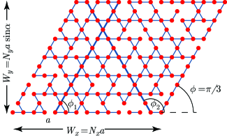
Figure 1: A bond-diluted kagome lattice with $p=0.8$ and $N_{x}=14$ horizontal bonds and $N_{y}=12$ bonds along the axis at an angle $\alpha=\pi/3$ to the $x$-axis. The red sites on the lattice are crosslinks, and colinear sequences of bonds are filaments. Only two filaments, shown with thicker bonds, traverse the lattice from top to bottom and support external stresses. One these makes an angle $\phi_{1}=\pi/3=\alpha$ and one an angle $\phi_{2}=2\pi/3=2\alpha$ with the $x$-axis, and the length of both is $N_{y}a$. In more general lattices, sample crossing filaments can orient at any angle $\phi$ to the $x$-axis, but the projection of their length onto the vertical axis is $W_{y}$, and thus their length is $L(\phi)=W_{y}/(a\sin\phi)$.

The building blocks of filamentous networks are typically semi-flexible polymers, characterized by a bending modulus $\kappa=l_{p}k_{B}T$, where $l_{p}$ is the persistence length $k_{B}$ the Boltzmann constant, and $T$ the temperature. Where filaments intersect, physical or chemical crosslinks bind them together but do not inhibit their relative rotation. Since only two filaments cross at a point, each crosslink is connected to at most four others. The average distance $l_{c}$ between crosslinks is less that $l_{p}$. A remarkably faithful description of experimentally measured linear MacKintosh et al. (1995); Peichocka et al. (2012) and nonlinear Storm et al. (2005) elastic response is provided by a model in which elastic response is assumed to be affine and in which filamentous sections between crosslinks are treated as nonlinear central-force springs with a force-extension curve determined by the worm-like chain model MacKintosh et al. (1995); Marko and Siggia (1995); Storm et al. (2005) augmented by an enthalpic stretching energy. This simple model, however, misses some important properties of filamentous networks, including the existence of a rigidity percolation threshold Feng and Sen (1984); Jacobs and Thorpe (1995), nonaffine response Onck et al. (2005); Heussinger and Frey (2006); Heussinger et al. (2007); Huisman et al. (2008), and crossover from bending-dominated nonaffine response at small $L/l_{c}$ Head et al. (2003a, b), or low frequency Huisman et al. (2010), to almost affine, stretching dominated response at large $L/l_{c}$ or high frequency.

The Mikado model Wilhelm and Frey (2003); Head et al. (2003b) provides additional insights into the physics of filamentous networks. In this model, straight filaments of length $L$ are deposited with random position and orientation on a two-dimensional flat surface and crosslinked at their points of intersection. Filaments are treated as elastic rods with one-dimensional stretching and bending moduli, $\mu$ and $\kappa$, rather than as worm-like chains. Numerical simulations on this model reveal a rigidity percolation transition from a floppy network to one with non-vanishing shear and bulk moduli and with non-affine bending dominated elastic response. As $L/l_{c}$ is increased, response becomes more affine and stretching dominated, reaching almost perfectly affine response in the $L/l_{c}\rightarrow\infty$ limit. Our EMTs and numerical simulations yield similar results for the diluted kagome model.

Though the Mikado and the diluted kagome lattice are quite similar with crosslinks of maximum coordination four and variable values of the ratio $L/l_{c}$, they model slightly different parts of the phase space of possible two-dimensional filamentous networks. In particular, since the starting point of the diluted kagome lattice is the full lattice with all bonds occupied, it necessarily deals directly with the $L\rightarrow\infty$ limit, which is not generally accessed in studies of the Mikado model in which $L$ is restricted to be less than the sample width $W$. The Mikado model is an “off-lattice” model, whereas the kagome model is lattice based. The latter property of the kagome model facilitates the application of lattice-based EMTs Soven (1969); Kirkpatrick et al. (1970); Elliott et al. (1974) (modified to include bending) for all values of $p$. Finally, In the Mikado model, the distance between between crosslinks on a single filament follows a Poisson distribution with no lower bound, whereas in the kagome lattice, this distance is an integral multiple of the lattice spacing with a lower bound of one lattice spacing. This difference leads, as we shall see, to a different scaling of the shear modulus in the bending dominated regime near $p=1$.

As detailed in Apps. B and C, our EMTs clearly show that there are three critical points (or fixed points in the renormalization-group sense): the trivial empty lattice point at $p=0$ (which we ignore), the rigidity-percolation point at $p=p_{b}$, and the $p=1$ full lattice point. It also provides analytic scaling relations for the the shear modulus $G$ as a function of $\mu$, $\kappa$, and $p$ in the $W\rightarrow\infty$ limit near both $p=p_{b}$ and $p=1$. Of particular interest is the behavior near $p=1$, where the ratio $G/G_{0}$ of the shear modulus to its $p=1$ value $G_{0}$ can be expressed as a function of the single scaling variable

$$\tau=\frac{\kappa}{(1-p)^{2}\mu a^{2}}\sim\frac{l_{b}^{2}\langle L\rangle^{2}}{l_{c}^{4}},$$ (1)

where $l_{b}^{2}=\kappa/\mu$ is the bending length $\langle L\rangle=a/(1-p)$ is the average filament length and $l_{c}\approx a$ is the average spacing between crosslinks along a filament. As $\tau\rightarrow\infty$, $G$ approaches $G_{0}$, but as $\tau\rightarrow 0$, there is crossover to a bending dominated, nonaffine regime in which

$$G\propto\frac{\kappa}{l_{c}^{3}}\frac{\langle L\rangle^{2}}{l_{c}^{2}}.$$ (2)

This behavior, which appears in our simulations, has also been observed in simulations in diluted three-dimensional lattices of four-fold coordinated filaments Stenull (2011); Broedersz et al. (2012). In Sec. V, we speculate about the reasons for the same behavior appearing in both two- and three-dimensions. Huessinger et al. Heussinger and Frey (2006); Heussinger et al. (2007) developed an off-lattice EMT for filamentous networks that predicts a bending-dominated non-affine regime with a different power of $L/l_{c}$, $G\sim(\kappa/l_{c}^{3})(L/l_{c})^{4}$, than the one we predict. The origin of this different scaling is the absence of a lower cutoff in the Poisson distribution of the distance between crosslinks in the Mikado model compared to the fixed cutoff equal to the lattice spacing in the kagome model. The analysis of Refs. Heussinger and Frey (2006); Heussinger et al. (2007) yields the kagome lattice scaling law if the probability distribution for distances is replaced by one with a fixed lower cutoff.

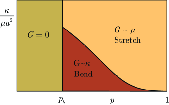
Figure 2: Schematic phase diagram for the diluted kagome lattice showing the bending-dominated region in which $G\sim\kappa$ and the stretching dominated region in which $G\sim\mu$. This boundary between stretching- and bending-dominated response was calculated using a formula that interpolates between the analytic EMT expressions for $G$ near $p=p_{b}$ and near $p=1$.

Our numerical simulations follow the EMT prediction very closely with no adjustable parameters near $p=1$ if $\kappa$ is not too large. For really small values of $\kappa/\mu a^{2}$, finite-size effects become important, and simulations can be fit with a combination of the exactly calculable finite size results at $\kappa=0$ and the EMT scaling form valid at infinite $W$. Near $p=p_{b}$, simulations are consistent with a scaling function of the form of Eq. (LABEL:EQ:scaling-2) but with $t$ approximately $0.2$ rather than $1$ and with different values of $c_{1}$ and $c_{2}$.

Under periodic boundary conditions, the kagome lattice has exactly $z=4=2d$ neighbors per site, where $d$ is the spatial dimension. If sites interact only via central-force springs on bonds and not by bending forces along filaments, the lattice is isostatic in that it has exactly enough internal forces to eliminate zero modes according the simple Maxwell count Maxwell (1864): $N_{0}=dN-N_{B}=(d-\frac{1}{2}z)N$, where $N_{0}$ is the number of zero modes and $N_{B}=\frac{1}{2}zN$ is the number of bonds. Under free rather than periodic boundary conditions, sites on the boundaries have fewer than four neighbors, and there is an overall bond deficiency of $\Delta N_{B}=2N-N_{B}\sim\sqrt{N}$. As a result, there are of order $\sqrt{N}$ zero “floppy” internal modes of zero energy in the absence of bending forces. Under periodic boundary conditions, the simple Maxwell count leads to $N_{0}=0$, but the total number of zero modes (as calculated by the dynamical matrix, whose normal modes are the “infinitesimal” modes that result when the elastic energy is truncated to harmonic order), like the number under free boundary conditions, is of order $\sqrt{N}$ rather than zero Souslov et al. (2009). This discrepancy is a result of the existence of lattice configurations that can support stress in bonds while maintaining a zero force at each note Sun et al. (2012). Associated with each such configuration Calladine (1978), called a “state of self stress”, is an additional infinitesimal zero mode so that the Maxwell count becomes $N_{0}=dN-N_{B}+S$, where $S$ is the number of states of self stress. Thus, in the undiluted central-force kagome lattice under periodic boundary conditions, $N_{0}=S$ is simply the number of states of self-stress. These states endow the undiluted central-force kagome lattice with affine response and non-zero bulk and shear moduli, proportional to the bond spring constant, and, thus, determine the approach to affine, stretching-dominated response as $p\rightarrow 1$ in the diluted lattice with nonzero $\kappa$. In addition, the central-force zero modes associated with the states of self stress also control the form of the effective-medium equations and the scaling forms they predict. The addition of bending forces lifts all but the two trivial zero modes of rigid translation to finite frequency. This fact plays a central roll in our EMT and is ultimately responsible for the form of the scaling function for $G$ near $p=1$.

We are ultimately interested in three-dimensional filamentous networks, which are subisostatic with $N_{0}=3N-2N=N$ because their maximum coordination number, like the that of two-dimensional networks, is four. If constituent filaments are straight, these networks have a state of self-stress for each filament in the undiluted limit, and their elastic moduli are non-zero, proportional to the bond-spring constant, and independent of $\kappa$ Stenull (2011). Associated with each state of self-stress, there is an additional zero mode, but as in the kagome lattice, the addition of bending forces raises all but the three trivial zero modes of uniform translation to finite frequency and stabilizes the lattice. We will argue in Sec. V that these properties are the likely origin of the very similar behavior, seen in simulations, of the shear modulus in $2$- and $3$-dimensional networks with maximum coordination of four.

This paper consists of five sections and three appendices. Section II compares and contrasts the Mikado and kagome models and demonstrates how straight, sample-traversing filaments with the energy of an elastic beam produce affine elastic response. Section II also defines the lattice model that we use. Section III describes EMT procedures and presents their results. Section IV presents the results of our numerical simulations and compares them with those of the EMTs. Section V reviews our results and speculates about application of our two-dimensional calculations to three-dimensional systems. There are three appendices: Appendix A discusses general properties of the EMT dynamical matrix. Appendices B and C present details of the solutions to the EMT equations near $p=1$ and $p=p_{b}$ for the bending EMTs described in Refs. Broedersz et al. (2011); Mao et al. (2011) and in Refs. Das et al. (2007, 2012), respectively.

II Filamentous networks and the diluted kagome lattice

Networks composed of straight filaments with elastic-rod energies have special properties. In this section, we will explore some general properties of these networks before setting up the energy for the kagome lattice.

II.1 Elastic filamentous networks

The elastic energy of a one-dimensional elastic beam with stretching modulus $\mu$ and bending modulus $\kappa$ is

$$E_{\text{fil}}=\frac{1}{2}\mu\int_{0}^{L}ds\left(\frac{du(s)}{ds}\right)^{2}+\frac{1}{2}\kappa\int_{0}^{L}ds\left(\frac{d\theta(s)}{ds}\right)^{2},$$ (3)

where $u(s)$ is the local longitudinal displacement and $\theta(s)$ the local angle of the tangent to the filament at the point $s$. The usual practice is to treat the stretching modulus as independent of $\kappa$ even though at nonzero temperature the spring constant for the entire filament has an important entropic component that depends on $\kappa$ .

The spring constant for a filament section of length $l$ is $k=\mu l^{-1}$. This leads to affine response in linear elasticity for any lattice in any dimension consisting of sample-traversing straight filaments with a sufficient number of orientations to ensure stability with respect to all strain Heussinger and Frey (2006); Heussinger et al. (2007); Gurtner and Durand (2009). To see this, consider a crosslink (node of the lattice) at the origin on a filament parallel to the unit vector $\mathbf{e}$, and let it be connected to two other crosslinks on the same filament at respective positions $\mathbf{s}_{1}=l_{1}\mathbf{e}$ and $\mathbf{s}_{1}=-l_{2}\mathbf{e}$ relative to the orign. Under a uniform, affine deformation, the relative positions $\mathbf{s}_{a}$, $a=1,2$ transform to $\Lambda\cdot\mathbf{s}_{a}\equiv\mathbf{s}_{a}+\eta\cdot\mathbf{s}_{a}$ , where $\Lambda=I+\eta$ is the deformation tensor with components $\Lambda_{ij}=\delta_{ij}+\eta_{ij}$. The forces that crosslinks $1$ and $2$ exert on the origin are then

$$\mathbf{f}_{1}=k(l_{1})(l_{1}e_{i}\eta_{ij}e_{j})\mathbf{e};\,\,\,\,\,\,\mathbf{f}_{2}=-k(l_{2})(l_{2}e_{i}\eta_{ij}e_{j})\mathbf{e},$$ (4)

where $i$ and $j$ run over $x,y$ and the summation convention is understood. The sum of these forces is zero because $k(l)=\mu/l$. The same analysis applies to any site and filament in the lattice. Under affine distortions, filaments do not bend, so the energy of the affine distortion depends only on the central force and does not depend on $\kappa$. Thus, under affine distortions of sample traversing filaments, the force on every intermediate crosslink is zero, and non-affine distortions are not introduced: the response is affine and independent $\kappa$. When the lattice is diluted, not every crosslink is connected to two others, the above cancelation does not occur, and the result is nonaffine response with a bending component.

With these observations, we can calculate the shear modulus of any network of straight filaments with stretching energy only, i.e., $\kappa=0$. For simplicity, we restrict our attention to two-dimensional systems in a rectangular- or rhombus-shaped box with base-length $W_{x}$ and height $W_{y}$ as shown in Fig. 1, and we consider only shear deformations in which the only nonvanishing component of $\eta$ is $\eta_{xy}$. In this case, only those filaments that cross from the bottom to the top of the sample will contribute to the shear modulus. The length of such a sample traversing filament oriented along a unit vector $\mathbf{e}(\phi)=(\cos\phi,\sin\phi)$ making an angle $\phi$ with the $x$-axis is $L(\phi)=W_{y}/(a\sin\phi)$. Under a shear deformation $\eta$, its length will change by $\delta L=Le_{i}(\phi)\eta_{ij}e_{j}(\phi)$ to lowest order in $\eta$. Since the spring constant of a filament of length $L$ is $\mu/L$, the elastic energy of the filament is

$$E_{\text{fil}}(\phi)=\frac{1}{2}\mu W_{y}\frac{[e_{i}(\phi)\eta_{ij}e_{j}(\phi)]^{2}}{\sin\phi}.$$ (5)

and the total energy from all filaments is $E_{\text{tot}}=(1/2)NW_{y}\mu\langle[e_{i}(\phi)\eta_{ij}e_{j}(\phi)]^{2}/\sin\phi\rangle$, where $N$ is the total number of sample traversing filaments and $\langle\cdots\rangle$ signifies an average over the orientation angles of the filaments.

The linearized energy density, $E/W_{x}W_{y}$, is

$$f=\textstyle{\frac{1}{2}}\,C_{ijkl}\,u_{ij}u_{kl}\,,$$ (6)

where $C_{ijkl}$ are the components of the elastic constant or elastic modulus tensor and $u_{ij}=\textstyle{\frac{1}{2}}(\eta_{ij}+\eta_{ji})$ are the components of the linearized strain tensor $\underline{\underline{\hat{u}}}$. In the isotropic limit, the energy density reduces to

$$f=\frac{1}{2}B\big{(}\textrm{Tr}\underline{\underline{u}}\big{)}^{2}+G\textrm{Tr}\underline{\underline{\hat{u}}}^{2},$$ (7)

where $\underline{\underline{\hat{u}}}$ is the traceless part of $\underline{\underline{u}}$, and $G=C_{xyxy}$ and $B=\textstyle{\frac{1}{2}}(C_{xxxx}+C_{xxyy})$ are the shear and bulk moduli, respectively. These relations along with Eq. (5) for the case in which the only nonvanishing component of $\eta_{ij}$ is $\eta_{xy}$ lead to

$$G=\frac{1}{4}\frac{\mu N}{W_{x}}\left\langle\frac{\sin^{2}2\phi}{\sin\phi}\right\rangle$$ (8)

for the shear modulus of a network of elastic rods with stretching modulus $\mu$. Note that rods parallel to the $x$-axis ($\phi=0$) do not contribute to $G$. In the kagome lattice, bottom-to-top traversing filaments all have length $L_{y}=W_{y}/\sin(\pi/3)$ and their angles with respect to the $x$-axis are restricted to $\phi=\pi/3,2\pi/3$ for which $\sin\phi=\sin 2\phi=\sqrt{3}/2$. There are $W_{x}/a$ sites along the $x$ axis from which a single filament aligned either along $\pi/3$ or $2\pi/3$ can emerge, so $N$ is simply $q_{\text{cross}}W_{x}/a$, where $q_{\text{cross}}(p)$ is the probability a filament emerging from a given site along the $x$-axis traverses the sample. For simplicity, we take $L_{y}=W$ in which $q_{\text{cross}}(p,W)=p^{W/a}$. When $p=1$, all bonds are occupied, and the shear modulus of the undiluted kagome lattice is $G_{0}=(\sqrt{3}/8)(\mu/a)$. When $p<1$ and $\kappa=0$, there is a nonzero stretching contribution to $G$ in finite samples:

$$G_{\text{str}}(\mu,p,W)\equiv G(\mu,\kappa=0,p,W)=q_{\text{cross}}(p,W)G_{0}.$$ (9)

In the $W\rightarrow\infty$ limit, the probability of sample traversing filaments vanishes for any $p<1$, and $G_{\infty}(\mu,\kappa,p)=\lim_{W\rightarrow\infty}G(\mu,\kappa,p,W)$ is zero at $\kappa=0$ for all $p<1$. Thus, as $\kappa\rightarrow 0$, $G_{\infty}(\mu,\kappa,p)$ must become smaller than $G_{\text{str}}(\mu,p,W)$, and for sufficiently small $\kappa$ and $p$ near one, $G(\mu,\kappa,p,W)\approx G_{\text{str}}(\mu,p,W)$, and, as we will show in Sec. IV, the simple interpolation formula

$$G(\mu,\kappa,p,W)\approx\max\{G_{\infty}(\mu,\kappa,p),G_{\text{str}}(\mu,p,W)\}$$ (10)

provides and excellent description of the simulation data with the EMT form for $G_{\infty}$ near $p=1$ where the finite size corrections are the most important.

II.2 Kagome lattice energy

The kagome lattice has three sites per unit cell, which we take to be the three sites, labeled $1$, $2$, and $3$, on an elemental triangle in Fig. 3. All bonds in the lattice are parallel to one of the vectors, $\mathbf{e}_{1}$, $\mathbf{e}_{2}$, and $\mathbf{e}_{3}$, specifying the direction of bonds in the unit elemental triangle. We label each site by an index $\ell=(\mathbf{l},\sigma)$ where $\mathbf{l}=(l_{1},l_{2})$ labels the position of site $1$ in the unit cell at dimensionless (i.e., taking $a=1$) position $\mathbf{r}_{\mathbf{l}}=2(l_{1}\mathbf{e}_{1}+l_{2}\mathbf{e}_{2})$, where the factor of two arises because the separation between unit cells is twice the bond length. The index $\sigma=1,2,3$ labels the site within the unit cell, and the position of site $\ell$ is $\mathbf{r}_{\ell}=\mathbf{r}_{\mathbf{l}}+\mathbf{s}_{\sigma}$, where $\mathbf{s}_{1}=0$, $\mathbf{s}_{2}=\mathbf{e}_{1}$, and $\mathbf{s}_{3}=-\mathbf{e}_{3}$. When the lattice is distorted, $\mathbf{r}_{\ell}$ maps to a new position $\mathbf{R}_{\ell}=\mathbf{r}_{\ell}+\mathbf{u}_{\ell}$, where $\mathbf{u}_{\ell}$ is the displacement vector of site $\ell$. The stretching energy of a bond $\langle\ell,\ell^{\prime}\rangle$ connecting nearest-neighbor ($NN$) sites $\ell$ and $\ell^{\prime}$ is $(1/2)(\mu/a)(\mathbf{u}_{\ell\ell^{\prime}}\cdot\hat{\mathbf{r}}_{\ell\ell^{\prime}})^{2}$ where $\mathbf{u}_{\ell\ell^{\prime}}=\mathbf{u}_{\ell^{\prime}}-\mathbf{u}_{\ell}$ and $\hat{\mathbf{r}}_{\ell\ell^{\prime}}$ is the unit vector parallel to $\mathbf{r}_{\ell^{\prime}}-\mathbf{r}_{\ell}$. Bending energy is determined by angles $\theta_{\ell\ell,\ell^{\prime\prime}}$ between $NN$ contiguous bonds $\langle\ell,\ell^{\prime}\rangle$ and $\langle\ell^{\prime},\ell^{\prime\prime}\rangle$ parallel to one of the lattice directions $\mathbf{e}_{n}$. To harmonic order, $\theta_{\ell\ell^{\prime}\ell^{\prime\prime}}=(1/a)(\mathbf{u}_{\ell\ell^{\prime}}-\mathbf{u}_{\ell^{\prime}\ell^{\prime\prime}})\cdot\mathbf{e}^{\perp}_{n}$, where $\mathbf{e}^{\perp}_{n}$ is the vector perpendicular to $\mathbf{e}_{n}$, which specifies the directions of both bonds $\langle\ell,\ell^{\prime}\rangle$ and $\langle\ell^{\prime},\ell^{\prime\prime}\rangle$, according the right hand rule about the outward normal to the plane. The bending energy arising from a nonzero $\theta_{\ell\ell^{\prime}\ell^{\prime\prime}}$ is $(1/2)(\kappa/a^{3})(\theta_{\ell\ell^{\prime}\ell^{\prime\prime}})^{2}$, and the harmonic energy for our latticed is thus

$$E = E_{s}+E_{b}$$ (11a)

$$E_{s}(\mu) = \frac{1}{2}\frac{\mu}{a}\sum_{\langle\ell,\ell^{\prime}\rangle}g_{\ell,\ell^{\prime}}(\mathbf{u}_{\ell\ell^{\prime}}\cdot\hat{\mathbf{r}}_{\ell\ell^{\prime}})^{2},$$ (11b)

$$E_{b}(\kappa) = \frac{1}{2}\frac{\kappa}{a}\sum_{\ell,\ell^{\prime},\ell^{\prime\prime}}g_{\ell,\ell^{\prime}}g_{\ell^{\prime},\ell^{\prime\prime}}(\theta_{\ell\ell^{\prime}\ell^{\prime\prime}})^{2}$$

$$= \frac{1}{2}\frac{\kappa}{a^{3}}\sum_{\langle\ell,\ell^{\prime},\ell^{\prime\prime}\rangle}g_{\ell,\ell^{\prime}}g_{\ell^{\prime},\ell^{\prime\prime}}\big{[}(\mathbf{u}_{\ell\ell^{\prime}}-\mathbf{u}_{\ell^{\prime}\ell^{\prime\prime}})\cdot\mathbf{e}^{\perp}_{n}\big{]}^{2},$$

where $g_{\ell,\ell^{\prime}}=1$ if the bond connecting sites $\ell$ and $\ell^{\prime}$ is occupied and $g_{\ell,\ell^{\prime}}=0$ otherwise and where the sum in $E_{b}(\kappa)$ is over all continuous triples of sites $\ell,\ell^{\prime},\ell^{\prime\prime}$ along each filament. The combination $\mu/a$ is the stretching elastic constant, and the combination $\kappa/a^{3}$ is the bending constant for contiguous pairs of bonds.

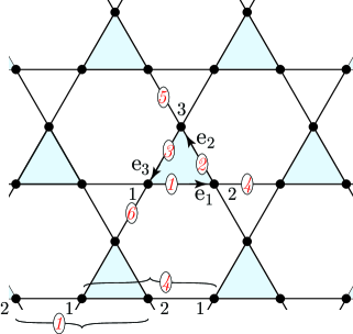
Figure 3: A section of a kagome lattice showing lattice directions $\mathbf{e}_{1}$, $\mathbf{e}_{2}$, and $\mathbf{e}_{3}$. Sites and $NN$ bonds in our choice for the unit cell labeled $1$, $2$, and $3$ and $1-6$ in italics, respectively. Two of the six $NNN$ bonds in a unit cell are shown at the bottom of the figure. The other four have a similar configurations aligned along $\mathbf{e}_{2}$ and $\mathbf{e}_{3}$ rather than $\mathbf{e}_{1}$.

III EMT: Overview and Results

Effective medium theory Soven (1969); Kirkpatrick et al. (1970); Elliott et al. (1974) is a well-established approximation for calculating properties such as electronic band structure and phonon or magnon dispersions of random media. Various formulations of EMT exist, but all replace the random medium with a homogeneous one whose parameters (such as $NN$ hopping strength or spring constant) are determined by a self-consistent equation. Here we use the formulation, presented in greater detail in App. A, in which self-consistency equations for the effective-medium parameters are determined by requiring that the average multiple-scattering potential or $T$-matrix associated with a single random bond (or group of bonds) in the homogeneous effective medium vanishes.

The development of an EMT for elastic networks with both stretching and bending forces presents challenges not encountered in networks with stretching forces only. In our system, stretching forces are associated with single $NN$ bonds, but bending forces are associated with contiguous pairs of $NN$ bonds that couple next-nearest-neighbor ($NNN$) sites in what we call phantom $NNN$ bonds that only exist if both its constituent $NN$ bonds are occupied. Thus, the replacement of a single $NN$ bond, which we will refer to as the replacement bond, in an effective medium affects not only the stretching energy of that bond but also the bending of the two $NNN$ “phantom” bonds containing that bond. There are currently two versions Das et al. (2007); Broedersz et al. (2011); Mao et al. (2011); Das et al. (2012) of EMT on lattices with bending energies, which we will refer to as EMT I and EMT II, respectively, that deal with this problem in different ways. In both methods, the effective medium is characterized by homogeneous stretching and bending moduli $\mu_{m}$ and $\kappa_{m}$ respectively.

In EMT I Broedersz et al. (2011); Mao et al. (2011), the replacement bond has a stretching modulus $\mu_{s}$ and a bending modulus $\kappa_{s}$ that take on respective values $\mu$ and $\kappa$ if the bond is occupied and $0$ if the bond is not occupied. Thus, the probability distribution for $\mu_{s}$ and $\kappa_{s}$,

$$P(\mu_{s},\kappa_{s})=p\delta(\mu_{s}-\mu)\delta(\kappa_{s}-\kappa)+(1-p)\delta(\mu_{s})\delta(\kappa_{s}),$$ (12)

exhibits strong correlation between the values of $\mu_{s}$ and $\kappa_{s}$. As discussed in detail in Ref. Mao et al. (2011), the bending constant of the $NNN$ phantom bonds containing the replacement bond is calculated assuming it is composed of two elastic beams connected in series, one with the bending modulus $\kappa_{m}$ of the effective medium and one with the bending modulus $\kappa_{s}$ of the replacement bond. This leads to a bending constant, $\kappa_{c}$, for both $NNN$ bond containing he replacement bond, that is a nonlinear function of $\kappa_{s}$ and $\kappa_{m}$:

$$\kappa_{c}(\kappa_{s})=2\left(\frac{1}{\kappa_{s}}+\frac{1}{\kappa_{m}}\right)^{-1}.$$ (13)

The perturbation to the effective medium arising from the replacement bond then consists of a stretching energy on that bond with spring constant $(\mu_{s}-\mu_{m})/a$ and bending constants on the two $NNN$ bonds of $(\kappa_{c}-\kappa_{m})/a^{3}$. It turns out, as discussed more fully in Refs. (Broedersz et al. (2011); Mao et al. (2011)) and in App. B, that the EMT equations in Method I do not close unless an additional term, with coupling constant $\lambda_{m}$, coupling the angles on neighboring $NNN$ bonds along a single filament is added to the effective medium energy. This leads to an additional term in the perturbation arising from the replacement bond, with coupling constant $-\lambda_{m}/a^{3}$, that couples the two angles on the two $NNN$ bonds containing the replacement bond. Thus this EMT is characterized by three parameters $\mu_{m},\kappa_{m}$, and $\lambda_{m}$.

In EMT II Das et al. (2007, 2012), the phantom $NNN$ bonds carrying the bending energy are elevated to the status of real bonds that exist whether or not the $NN$ bonds of which they are composed are occupied. This leads to the great simplification that stretching and bending are effectively decoupled, and there is no necessity of introducing $\lambda_{m}$. There are separate probability distributions for the stretching modulus of the $NN$ replacement bond and for the bending modulus of the $NNN$ replacement bond. However, since the bending modulus of a $NNN$ bond is zero unless both $NN$ bonds comprising it are occupied, the probability that the $NNN$ is present with a bending modulus $\kappa$ is chosen to be $p^{2}$, the probability that any two given $NN$ bonds are occupied:

$$P(\mu_{s}) = p\delta(\mu_{s}-\mu)+(1-p)\delta(\mu_{s})$$ (14a)

$$P(\kappa_{s}) = p^{2}\delta(\kappa_{s}-\kappa)+(1-p^{2})\delta(\kappa_{s}).$$ (14b)

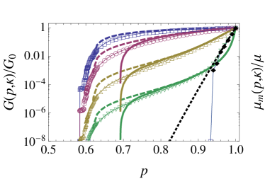
Figure 4: Comparison between the shear modulus (normalized by the shear modulus $G_{0}$ at $p=1$, so it is equivalent to $\mu_{m}/\mu$) obtained from our numerical simulations (data points): EMT I (solid lines) and EMT II (dashed lines). Different colors mark different values of $\kappa/(\mu a^{2})$, and from top to bottom the corresponding values of $\kappa/(\mu a^{2})$ are $1$, $10^{-2},10^{-4},10^{-6}$, $0$. The dotted line indicates the finite size correction predicted by Eq. (10) As $p$ increases toward $1$ the simulation curve for $\kappa/(\mu a^{2})=10^{-6}$ follows first the EMT curves and then the finite-size $\kappa=0$ curve beyond the point at which the latter curves meet in accord with Eq. (10). For the values of $\kappa/(\mu a^{2})>10^{-6}$, the EMT solution is larger that the $\kappa=0$ finite-size result, and thus the simulation data follow the EMT curves.

The predictions of these two methods are qualitatively similar: they both yield a rigidity percolation threshold, below which the lattice loses rigidity, and a smoothly varying shear modulus approaching the pure lattice value of $G_{0}$ as $p\rightarrow 1$. Figure 4 plots values of $G(k,\kappa)$ calculated using both EMT methods for different values of $\kappa/(\mu a^{2})$ and $p$ along with the results of simulations. The $\kappa=0$ simulation curves follows the finite-size result of Eq. (9). The $\kappa/(\mu a^{2})=10^{-6}$ curve follows the EMT curve, which corresponds to infinite $W$, with increasing $p$ and then the $\kappa=0$ finite size curve after the two cross in accord with Eq. (10). As is the case for the triangular lattice Das et al. (2012), EMT II predicts a value of $p_{b}$ that is close to that measured in simulations, whereas EMT I predicts a considerably larger value. In addition, for values of $\kappa/(\mu a^{2})$ beyond $0.1$, the EMT I numerical solution ceases to exist for small $p$, and as a result the $\kappa/(\mu a^{2})=1$ curve is not included for EMT I in Fig. 4. For $p\gtrsim 0.7$ and $\kappa/(\mu a^{2})>10^{-6}$, the two EMT curves and the simulation curves are essentially indistinguishable, and near $p=1$, they become analytically identical with the effective medium modulus $\mu_{m}$ satisfying a scaling form

$$\mu_{m}=\mu\cdot\Psi(\tau)$$ (15)

where the scaling variable is

$$\tau=\frac{\kappa/(\mu a^{2})}{(1-p)^{2}}=\frac{\kappa}{\mu a^{4}}\langle L\rangle^{2}$$ (16)

and the scaling function is

$$\Psi(\tau) =(-1+\sqrt{1+A\tau})^{2}/(A\tau)\,.$$ (17)

with the constant $A=[40(1-\sqrt{2/3})]^{2}\simeq 53.9$. This scaling function can be expanded in the following limits

$$\Psi(\tau)\simeq\left\{\begin{array}[]{ll}1&\textrm{if $\tau\gg 1$}\\ A\tau/4&\textrm{if $\tau\ll 1$}\end{array}\right.$$ (20)

Therefore, for the case of $\tau\gg 1$ corresponding to $p$ near $1$ so that $\kappa/(\mu a^{2})\gg(1-p)^{2}$, the shear modulus is approximately

$$G=\frac{\sqrt{3}}{8}\frac{\mu_{m}}{a}\approx\frac{\sqrt{3}}{8}\frac{\mu}{a}=G_{0},$$ (21)

indicating that the macroscopic elastic response of the network is dominated by the stretching stiffness of the filaments and reaches the affine pure lattice limit as $p\rightarrow 1$, and we shall call this the “stretching dominated”elastic regime.

In the other limit $\tau\ll 1$ corresponding to smaller $\kappa$ or larger $1-p$ so that $\kappa/(\mu a^{2})\ll(1-p)^{2}$, we have the shear modulus

$$G\simeq A\frac{\sqrt{3}}{32}\frac{\kappa}{a^{3}(1-p)^{2}}=A\frac{\sqrt{3}}{32}\frac{\kappa}{a^{3}}\frac{L^{2}}{a^{2}},$$ (22)

indicating that the macroscopic elastic response of the network is dominated by the bending stiffness of the filaments, and we shall call this the “bending dominated”elastic regime. The EMT solution for $p$ near one is plotted in terms of the scaling variable $\tau$ together with the asymptotic scaling function $\Psi(\tau)$ in Fig. 5. Because the asymptotic solution (17) assumes small $(1-p)$, it requires very small $\kappa/(\mu a^{2})$ to make the regime $\Psi(\tau)\simeq A\tau/4$ visible. We conclude from this that the elasticity of the network is bending dominant as long as

$$\kappa/(\mu a^{2})\ll(1-p)^{2}.$$ (23)

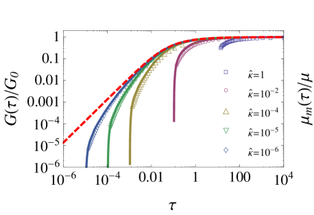
Figure 5: (Color online) Scaling behavior near $p=1$ for different values of $\hat{\kappa}\equiv\kappa/(\mu a^{2})$. The data points for the shear modulus stem from our simulations for $200^{2}$ unit cells. The continuous curves depict our numerical solutions for $\mu_{m}$ of the EMT equations for the corresponding values of $\kappa$. The dashed red curve shows the asymptotic scaling function predicted by the EMT, see Eq. (17). As expected, the simulation data and the numerical solution of the EMT equations deviate from this scaling function as $1-p$ becomes large.

As discussed in Sec. I, near the rigidity threshold, $G(p,\kappa)$ vanishes as $\mu(p-p_{b})^{t}$, where $t=1$ and $p_{b}=0.6920$ for EMT I and $p_{b}=0.6180$ for EMT II, times a scaling function of $b_{m}=\kappa/(\mu a^{2})$ that is a constant at large $b_{m}$ and proportional to $b_{m}$ at small $b_{m}$. Thus, at sufficiently small $b_{m}$ for all $p<1$, response is bending dominated with $G\propto\kappa$; at sufficiently large $b_{m}$, response is stretching dominated with $G\propto\mu$ as shown in the phase diagram of Fig. 2.

IV Numerical Simulations

In the numerical portion of our work, we study the elasticity of the filamentous kagome lattice by generating diluted lattice conformations on a computer and then calculating their mechanical response numerically. Practically this is done via deforming the network by imposing a certain $\eta$ and by then minimizing the elastic energy (11) over the non-affine displacements $\delta\mathbf{u}_{\ell}=\mathbf{u}_{\ell}-\eta\mathbf{r}_{\ell}$ of the sites using a conjugate gradient algorithm. To explore the response to shear, e.g., we set $\eta_{ij}=\gamma(\delta_{ix}\delta_{jy}+\delta_{iy}\delta_{jx})$, where $\gamma$ specifies the magnitude of the applied deformation. We use the same small magnitude $\gamma=0.01$ for all deformations. For a range of $p$-values, we generate up to $M=200$ random conformations, we calculate several measurable quantities for multiple $\kappa$-values, and we average arithmetically over all conformations. The quantities that we calculate are the elastic moduli and the corresponding fractions of rigid conformations $n_{ijkl}$ and non-affinity parameters $\Gamma_{ijkl}$. $n_{ijkl}$ is defined as the number of conformations with non-zero $C_{ijkl}$ (non-zero meaning larger than a small numerical threshold, here $10^{-8}$) divided by $M$. The non-affinity parameters DiDonna and Lubensky (2005)

$$\Gamma_{ijkl}=\frac{1}{N\gamma^{2}}\sum_{\ell}\left(\delta\mathbf{u}^{0}_{\ell}\right)^{2},$$ (24)

where $N$ is the total number of sites and $\delta\mathbf{u}^{0}_{\ell}$ is the equilibrium non-affine displacement of site $\ell$ in the presence of the $\eta$ that leads to $C_{ijkl}$, measure the deviation from a homogeneous strain field. To mitigate boundary effects, we apply periodic boundary conditions on all boundaries. We simulate system sizes ranging from $6^{2}$ to $200^{2}$ unit cells which corresponds to $N=108$ and $N=120,000$ sites, respectively.

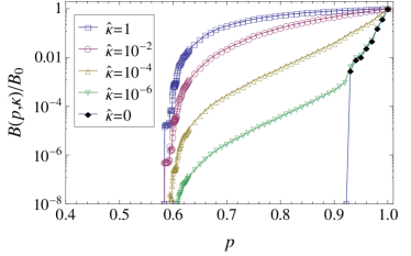
Figure 6: The bulk modulus $B$ (normalized by the bulk modulus $B_{0}$ at $p=1$) from our simulations of $48^{2}$ unit cells.

Figures 4 and 6 show log-linear plots of the shear modulus $G$ and the bulk modulus $B$, respectively, as functions of the occupation probability $p$ for $48^{2}$ unit cells. The EMT predicts the bulk modulus to be proportional to $\mu_{m}$, and hence, both $\mu$ and $B$ should follow the same curves when they are normalized by their respective affine values $G_{0}$ and $B_{0}$ at $p=1$. Within the numerical errors, this prediction is indeed borne out by Figs. 4 (a) and (b). Moreover, these figures are consistent with the EMT prediction that the rigidity percolation threshold $p_{b}$ be the same for all $\kappa>0$. Numerically, we find $p_{b}=0.605\pm 0.005$ which is only slightly smaller than the EMT II prediction $p_{b}\approx 0.616$ and about 15% smaller than the EMT I prediction $p_{b}\approx 0.692$. Previous EMT predictions for elastic networks have produced somewhat larger values for the rigidity threshold than found in corresponding numerical studies, see e.g., Refs. Broedersz et al. (2011); Mao et al. (2011), and this apparent trend is continued here. For $\kappa=0$, the EMT predicts a first-order rigidity percolation transition at $p=1$. The curves for $\kappa=0$ in Figs. 4 (a) and (b) rise from zero with finite slope below $p=1$, a clear finite-size effect. Below, we will analyze this finite-size effect systematically, and we will find that our data is indeed consistent with a first-order transition at $p=1$.

Figure 7 shows the non-affinity functions $\Gamma_{xyxy}$ and $\Gamma_{xxxx}$ extracted from the simulation runs producing the results for $\mu$ and $B$ discussed in the previous paragraph. For $p=1$, the network is affine, and the non-affinity functions are zero. The curves for $\kappa>0$ are expected to have their maxima at $p_{b}$, and our data is consistent with that expectation. The data for $\kappa=0$ the curves for $G$ and $B$ should show no indication of the existence of $p_{b}$, and indeed they do not.

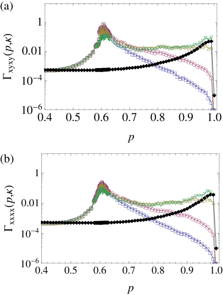
Figure 7: (Color online) Non-affinity ratios (a) $\Gamma_{xyxy}$ and (b) $\Gamma_{xxxx}$ for $48^{2}$ unit cells. Color-code is the same as in Figs. 4 and 6.

Next, we turn to the fractions of rigid conformations. These quantities are convenient for the purposes of finite-size analysis, in particular for the expected first-order transition for $\kappa=0$ at $p=1$. In the following, we will with focus on $n=n_{xyxy}$. Figure 8(a) displays $n$ for $48^{2}$ unit cells for $\kappa=0$ and several values of $\kappa>0$. The curves for $\kappa>0$ are consistent with the above statement that the rigidity percolation threshold for all non-vanishing values of $\kappa$ is at $p_{b}=0.605\pm 0.005$.

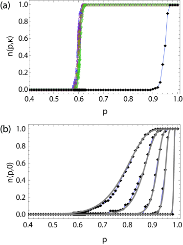
Figure 8: (Color online) Fraction of rigid conformations for (a) $48^{2}$ unit cells and various values of $\kappa$ [with the same color-code as in Figs. 4 and 6.], and (b) for $\kappa=0$ and system sizes of $S^{2}$ unit cells with $S=6,12,24,48,200$ (increasing from left to right). The bold lines correspond to the theoretical result (26).

Figure 8(b) shows $n$ for $\kappa=0$ for a variety of system sizes of $S^{2}$ unit cells. Along with the data points, the figure follows predictions for $n(\kappa=0,p,S)$ that follow from the elementary combinatorics (see Sec. II.1). Consider a system such as that shown in Fig. 1 with $N_{x}=2S$ bonds along its two sides. Only those filaments, which consist of $N_{x}$ bonds, that extend from the top to the bottom of the sample will contribute to $G$, and $G$ will be zero unless at least one of the filaments starting on bottom reaches the top, which occurs with probability

$$P_{\text{fil}}(p,N_{x})=1-(1-p^{N_{x}})^{N_{x}}.$$ (25)

This function becomes a step function at p=1 when $N_{x}\rightarrow\infty$. Thus, we expect the data for $\kappa=0$ to be fit by the function

$$n(\kappa=0,p,S)=P_{\text{fil}}(p,2S).$$ (26)

Figure 8 (b) reveals that the data is fit by this prediction remarkably well even though there is not a single adjustable fit-parameter involved. Now, we are in position to discuss the infinite-size limit. For $S\to\infty$, $n(\kappa=0,p,S)$ approaches a unit-step function at $p=1$. This establishes that the rigidity percolation transition for $\kappa=0$ is a first-order transition at $p=1$ where the shear modulus jumps discontinuously from zero to its affine value.

Now, let us look at the elastic response near $p=1$. Figure 5 shows the shear modulus and $\mu_{m}$ as functions of the scaling variable $\tau$ defined in Eq. (16). We find remarkably good agreement between the simulation data, the numerical solution of the EMT equations as well as the EMT prediction for the asymptotic scaling function $M(\tau)$ including the predicted value for the constant $A$. Note that this agreement is obtained without adjusting any fit-parameters.

Figure 9, finally, displays the scaling behavior near the rigidity percolation threshold $p_{b}$. Our numerical data collapses in full qualitative agreement with the EMT scaling form (LABEL:EQ:scaling-2) albeit with an exponent $t=0.2$ that is significantly smaller than the $t=1$ predicted by the EMT. The value $c_{1}=0.25$, on the other hand, is in semi-quantitative agreement with the EMT.

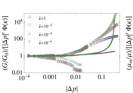
Figure 9: (Color online) Scaling behavior of the shear modulus near $p_{b}$. The plot shows both our simulation results and our numerical solutions of the EMT I equations relative to the asymptotic scaling form near $p_{b}$ predicted by the EMT, cf. Eq. (LABEL:EQ:scaling-2). The data points stem from our simulations for $48^{2}$ unit cells, and we use $p_{b}=0.605$, $c_{1}=0.3$, $c_{2}=0.007$, and $t=0.2$. The lower branches correspond to values of $p$ below $p_{b}$ and are a typical finite-size effect. The continuous curves represent the numerical solutions to the EMT I equations, which reduce to Eqs. (62) to(B.2) as $\Delta p$ tends to zero with $c_{1}=0.03802$, $c_{2}=4.697$, and $p_{b}=0.692$.

V Discussion

We have introduced the diluted kagome lattice in $2$-dimensions as a model for networks of semi-flexible polymers, whose maximum coordination number is four. We identify straight lines of contiguous occupied bonds as filaments that, following previous work Wilhelm and Frey (2003); Head et al. (2003a, b); Heussinger and Frey (2006); Heussinger et al. (2007); Huisman et al. (2008), we endow with the energy of an elastic beam characterized by a stretching (Young’s) modulus $\mu$ and a bending modulus $\kappa$. We contrast this model, which has filaments of arbitrary length, with the Mikado lattice whose filaments are of finite (and usually fixed length). We show that when $\kappa=0$, this kagome model has affine response and non-vanishing elastic moduli so long as there are sample-traversing filaments, which is the case for samples with finite lengths and widths $W$, even for bond-occupation probabilities $p$ less than one. As $W$ increases, the probability of sample-traversing filaments decreases, and in the $W\rightarrow\infty$ limit, elastic moduli, which are nonzero for undiluted $p=1$ lattice, fall precipitously to zero for $p=1^{-}$ in a first-order transition. The undiluted lattice has $\kappa$-independent, and thus affine, elastic moduli. The addition of bending forces restores rigidity for any $\kappa$ for $p$ greater than $p_{b}$, the rigidity percolation threshold, and elastic moduli approach the non-zero affine values of the $p=1$ lattice as $p\rightarrow 1$. We argue that this is the underlying cause for the affine limit found in the large $l/l_{c}$ limit ($p$ near one) in the Mikado model.

We use two recently introduced lattice-based effective medium theories to calculate elastic moduli of the diluted kagome lattice as a function of $\mu$, $\kappa$, and $p$, we we calculate scaling forms for the shear modulus both near $p=1$ and $p=p_{b}$. Both forms are a function of the unitless ratio $b_{m}=\kappa/(\mu a^{2})$, where $a$ is the lattice spacing, and yield a crossover for all $p_{b}<p<1$ between bending dominated response at small $b_{m}$ and stretching dominated response at large $b_{m}$. We supplement our EMTs with numerical simulations of the shear modulus and other functions, such as that measuring the degree of nonaffine response. The results of these simulations agree qualitatively with EMT predictions for all $p$ and quantitatively with them near $p=1$.

Our study of the kagome lattice provides insight into the behavior of $3$-dimensional filamentous lattices with maximum coordination number of four. With stretching forces only, these lattices are subisostatic with of order one zero mode per site, and one might, therefore, conjecture that their elastic moduli should vanish when $\kappa=0$. However, simulations Stenull (2011); Broedersz et al. (2012) on two model lattices consisting of straight filaments yields curves of elastic moudli as a function of $p$ that look very similar to those of the kagome lattice presented here with an approach to affine $\kappa$-independent response as $p\rightarrow 1$. The underlying cause of this result is that straight sample-traversing filaments in any dimension give rise to nonvanishing macroscopic elastic moduli. Indeed, exact calculations Stenull (2011) for one of the $3d$-lattices with elastic-beam energies show that all elastic moduli are nonzero when $\kappa=0$ and $p=1$ and that response is affine. Near $p=1$, simulations on both of the $3d$ lattice show a crossover from a bending dominated regime with $G\sim(\kappa/a^{3})(L/a)^{2}$ to a stretching dominated regime in which $G\sim\mu$ in agreement with the predictions of our kagome-based lattice EMT. In fact the results of one of the simulations Stenull (2011) track the scaling function of the our kagome EMT. We conjecture that the important common feature of the $2d$ and $3d$ lattices is that they both consist of sample-traversing straight filaments in the undiluted limit. Away from $p=1$, bending forces stabilize the lattices in a process that is not so sensitive to lattice dimension, even though the central-force $3d$ lattice is subisostatic. Our EMTs provide some support for this conjecture. The characteristic property of the kagome EMT solutions, such as the form of the scaling function near $p=1$, are a direct consequence of the existence of lines of zeros in the phonon spectrum at $\kappa=0$ that get raised to nonzero frequency for $\kappa>0$ as shown in Fig. 10. This feature causes the integral $H_{2,s}$ [Eqs. (B.1) to (57)] to diverge as $\sqrt{b_{m}}$ as $b_{m}=\kappa/(\mu a^{2})\rightarrow 0$. In three dimensions, the lines of zero modes in the phonon spectrum become planes of zero-modes, and we believe that the $3d$ version of $H_{2,s}$ will have a from analogous to Eq. (57) but with $g(q_{y})$ replaced by a similar function of $q_{y}$ and $q_{z}$:

$$H_{2,s}(b_{m},0) \sim\int d^{3}q\frac{|\langle\mathbf{B}_{1}^{b}|\nu_{f}\rangle|^{2}}{cq_{x}^{2}+b_{m}\tilde{g}(q_{y},q_{z})}$$

$$\sim b_{m}^{-1/2}.$$ (27)

When $b_{m}=0$, the denominator vanishes for all $q_{y}$ and $q_{z}$ when $q_{c}=0$, and the integral diverges. Nonzero $b_{m}$ yields a $b_{m}^{-1/2}$ divergence just as in the $2d$ kagome case. Unfortunately, the $3d$ lattices are quite complicated, with a $54$-site unit cell in one case Stenull (2011) and complicated crossing configurations in the other Broedersz et al. (2012), and we have not been able to set up a $3d$ EMT to verify this conjecture.

Much of the work on the elastic properties of filamentous networks (with the notable exceptions of Huisman et al. (2008, 2010); Huisman and Lubensky (2011)) have focused on models, such as the Mikado or kagome lattice presented her, consisting of straight filaments. This work has also largely focused on what are really mechanical models with beam energies assigned to the filaments and the effects of thermal fluctuations ignored. As our analysis shows, these are exceptional lattices because they can support stress with central forces only even when their coordination number $z$ is substantially less the Maxwell stability limit of $z=2d$. Filaments in real biological gels are not straight, and their energies are not described by that of an elastic beam. It is thus legitimate to ask how seriously one should take models such as those presented here as realistic descriptions of real bio-gels of semiflexible polymers. If constituent filaments are not straight, then in general, at least some of elastic moduli of even perfect lattices vanish in the absence of bending forces. Prime examples of this behavior are found in the two-dimensional honeycomb lattice and the three-dimensional diamond lattice whose bulk moduli are nonzero but whose shear moduli vanish in the $\kappa\rightarrow 0$ limit, but it has also been observed in a more realistic model of a filamentous lattice Huisman and Lubensky (2011). If $\kappa$ is needed to stabilize the system, the elastic response to external stresses will involve bending and thus be nonaffine. So, it would seem that the straight-filament models are not such good ones for real systems, though they do provide us with valuable insight into how network architecture influences elastic response. One of the predictions of the straight-filament models is that response becomes more stretching dominated and more affine as $\kappa$ increases. Thus, it is plausible that if $\kappa$ is large enough, the elastic response of even those lattices whose shear moduli vanish if $\kappa=0$ will exhibit stretching dominated, nearly affine response for sufficiently large $\kappa$.

Appendix A EMT Generalities and the EM Dynamical Matrix

To implement the $T$-matrix version of EMT, we deal with the dynamical matrix $\mathbf{D}^{m}$ of the EM, its associated Green’s funcition $\mathbf{G}^{m}=-(\mathbf{D}^{m})^{-1}$ (we consider only zero frequency), the perturbation $\mathbf{V}$ associated with bond replacement, the dynamical matrix $\mathbf{D}=\mathbf{D}^{m}+\mathbf{V}$, and its associated Green’s function $\mathbf{G}=-\mathbf{D}^{-1}$. [For more details of this formalism, see Refs. Mao and Lubensky (2011) and Mao et al. (2011)] Because there are three sites per unit cell, all of these matrices are $6N\times 6N$ matrices, to be detailed further below, where $N$ is the number of unit cells in the lattice. We will specify $\mathbf{G}^{m}$ more completely below. With these definitions,

$$\mathbf{G}=\mathbf{G}^{m}+\mathbf{G}^{m}\cdot\mathbf{T}\cdot\mathbf{G}^{m}=(\mathbf{G}^{m}-\mathbf{V})^{-1},$$ (28)

where

$$\mathbf{T}=\mathbf{V}\cdot(\mathbf{I}-\mathbf{G}^{m}\cdot\mathbf{V})^{-1}.$$ (29)

The EMT self-consistency equation requires that the disorder average over the probability distribution of Eq. (12) for EMT I or Eq. (14a) or EMT II of the perturbation vanishes

$$\langle\mathbf{T}(\mu_{s},\kappa_{s})\rangle=0.$$ (30)

All of the matrices discussed here can be expressed in a position or wavenumber representation. The six independent displacements in a unit cell can be expressed as a six-dimensional vector $\mathbf{U}_{\mathbf{l}}=(\mathbf{u}_{\mathbf{l},1},\mathbf{u}_{\mathbf{l},2},\mathbf{u}_{\mathbf{l},3})$ for each $\mathbf{l}$ or as its Fourier transform $\mathbf{U}_{\mathbf{q}}=\frac{1}{N}\sum_{\mathbf{l}}e^{-i\mathbf{q}\cdot\mathbf{r}_{\ell}}\mathbf{U}(\mathbf{l})=(\mathbf{u}_{\mathbf{q},1},\mathbf{u}_{\mathbf{q},2},\mathbf{u}_{\mathbf{q},3})$. The energy of the bond-replaced system is then

$$E = \frac{1}{2}\sum_{\mathbf{l},\mathbf{l}^{\prime}}\mathbf{U}_{\mathbf{l}}\mathbf{D}_{\mathbf{l},\mathbf{l}^{\prime}}\mathbf{U}_{\mathbf{l}}^{\prime}$$ (31)

$$= \frac{1}{2N^{2}}\sum_{\mathbf{q},\mathbf{q}^{\prime}}\mathbf{U}_{-\mathbf{q}}\mathbf{D}_{\mathbf{q},\mathbf{q}^{\prime}}\mathbf{U}_{\mathbf{q}^{\prime}},$$

where $D_{\mathbf{l},\mathbf{l}^{\prime}}$ and $\mathbf{D}_{\mathbf{q},\mathbf{q}^{\prime}}$ are $6\times 6$ dimensional matrices for each pair $(\mathbf{l},\mathbf{l}^{\prime})$ and $(\mathbf{q},\mathbf{q}^{\prime})$. The effective medium is translationally invariant and

$$\mathbf{D}^{m}_{\mathbf{q},\mathbf{q}^{\prime}}=N\delta_{\mathbf{q},\mathbf{q}^{\prime}}\mathbf{D}^{m}_{\mathbf{q}}.$$ (32)

The energy of the effective medium is constructed by occupying all bonds with identical beams with stretching and bending moduli $\mu_{m}$ and $\kappa_{m}$ and adding (for EMT I) an additional coupling of strength $\lambda_{m}$ coupling angles in neighboring $NNN$ bonds along a filaments [See Ref. Mao et al. (2011) for details]. The EM energy is then

$$E^{m} = E_{s}(\mu_{m})+E_{b}(\kappa_{m})+E^{m}_{bb}(\lambda_{m})$$ (33)

$$\equiv \frac{1}{2N}\sum_{\mathbf{q}}\mathbf{U}_{\mathbf{q}}\cdot\mathbf{D}^{m}_{\mathbf{q}}\cdot\mathbf{U}_{-\mathbf{q}}$$ (34)

where $E_{s}(\mu_{m})$ and $E_{b}(\kappa_{m})$ are evaluated at $g_{\ell,\ell^{\prime}}=1$ for all bonds $\langle\ell,\ell^{\prime}\rangle$, where

$$E^{m}_{bb}(\lambda_{m})=\frac{\lambda_{m}}{a^{3}}\sum_{\ell_{2},\ell_{3}}\theta^{n}_{\ell_{1},\ell_{2},\ell_{3}}\theta^{n}_{\ell_{2},\ell_{3},\ell_{4}},$$ (35)

where it is understood that $\ell_{1},\ell_{2},\ell_{3}$ and $\ell_{4}$ are all contiguous sites along a single filament. $\mathbf{G}^{m}_{\mathbf{q}}$ can be constructed from the Fourier transforms of the stretching and bending energies on $NN$ and phantom $NNN$ bonds. For example, the stretching energy of bond $5$ in Fig. 3, connecting site $\ell=(\mathbf{l},3)$ at position $\mathbf{r}_{\mathbf{l}}-\mathbf{e}_{3}$ with site $\ell^{\prime}=(\mathbf{l},2)$ at position $\mathbf{r}_{\mathbf{l}}+2\mathbf{e}_{2}+\mathbf{e}_{1}$ such that $\mathbf{r}_{\ell}^{\prime}-\mathbf{r}_{\ell}=\mathbf{e}_{2}$ is $\frac{1}{2}(\mu_{m}/a)[(\mathbf{e}_{\ell^{\prime}}-\mathbf{e}_{\ell})\cdot\mathbf{e}_{2}]^{2}$. The Fourier transform of $(\mathbf{e}_{\ell^{\prime}}-\mathbf{e}_{\ell})\cdot\mathbf{e}_{2}$ is

$$e^{-i\mathbf{q}\cdot\mathbf{l}}(e^{-i\mathbf{q}\cdot\mathbf{e}_{2}}\mathbf{u}_{2,\mathbf{q}}-\mathbf{u}_{3,\mathbf{q}})\cdot\mathbf{e}_{2}=e^{-i\mathbf{q}\cdot\mathbf{r}_{\mathbf{l}}}\mathbf{B}^{2}_{5,\mathbf{q}}\cdot\mathbf{U}_{\mathbf{q}},$$ (36)

where $\mathbf{B}^{2}_{5,\mathbf{q}}$ is specified in detail in Eq. (A) below. Similar procedures apply to all stretching and bending bonds, and the EM dynamical matrix can be expressed as

$$\mathbf{D}^{m}_{\mathbf{q}}\left(\mu_{m},\kappa_{m},\lambda_{m}\right)$$ (37)

$$= \frac{\mu_{m}}{a}\sum_{n=1}^{6}\mathbf{B}^{s}_{n,\mathbf{q}}\mathbf{B}^{s}_{n,-\mathbf{q}}$$

$$+\frac{\kappa_{m}}{a^{3}}\sum_{n=1}^{6}\mathbf{B}^{b}_{n,\mathbf{q}}\mathbf{B}^{b}_{n,-\mathbf{q}}$$

$$+\frac{\lambda_{m}}{a^{3}}\sum_{n=1}^{6}2\cos(\mathbf{q}\cdot\mathbf{e}_{n})\mathbf{B}^{b}_{n,\mathbf{q}}\mathbf{B}^{b}_{n,-\mathbf{q}},$$

where

$$\mathbf{B}_{1,\mathbf{q}}^{s} =\{-\mathbf{e}_{1},\mathbf{e}_{1},0,0\}$$

$$\mathbf{B}_{2,\mathbf{q}}^{s} =\{0,0,-\mathbf{e}_{2},\mathbf{e}_{2}\}$$

$$\mathbf{B}_{3,\mathbf{q}}^{s} =\{\mathbf{e}_{3},0,0,-\mathbf{e}_{3}\}$$

$$\mathbf{B}_{4,\mathbf{q}}^{s} =\{e^{-i\mathbf{q}\cdot\mathbf{e}_{1}}\mathbf{e}_{1},-\mathbf{e}_{1},0,0\}$$

$$\mathbf{B}_{5,\mathbf{q}}^{s} =\{0,0,e^{-i\mathbf{q}\cdot\mathbf{e}_{2}}\mathbf{e}_{2},-\mathbf{e}_{2}\}$$

$$\mathbf{B}_{6,\mathbf{q}}^{s} =\{-\mathbf{e}_{3},0,0,e^{-i\mathbf{q}\cdot\mathbf{e}_{3}}\mathbf{e}_{3}\}$$ (38)

and

$$\mathbf{B}_{1,\mathbf{q}}^{b} =2\{2\mathbf{e}^{\perp}_{1},-(1+e^{i\mathbf{q}\cdot\mathbf{e}_{1}})\mathbf{e}^{\perp}_{1},0,0\},$$

$$\mathbf{B}_{2,\mathbf{q}}^{b} =2\{0,0,2\mathbf{e}^{\perp}_{2},-(1+e^{i\mathbf{q}\cdot\mathbf{e}_{2}})\mathbf{e}^{\perp}_{2}\},$$

$$\mathbf{B}_{3,\mathbf{q}}^{b} =2\{-(1+e^{i\mathbf{q}\cdot\mathbf{e}_{3}})\mathbf{e}^{\perp}_{3},0,0,2\mathbf{e}^{\perp}_{3})\},$$

$$\mathbf{B}_{4,\mathbf{q}}^{b} =2\{-(1+e^{-i\mathbf{q}\cdot\mathbf{e}_{1}})\mathbf{e}_{1},-2\mathbf{e}_{1},0,0\},$$

$$\mathbf{B}_{5,\mathbf{q}}^{b} =2\{0,0,-(1+e^{-i\mathbf{q}\cdot\mathbf{e}_{2}})\mathbf{e}^{\perp}_{2},2\mathbf{e}^{\perp}_{2})\},$$

$$\mathbf{B}_{6,\mathbf{q}}^{b} =2\{2\mathbf{e}^{\perp}_{3},0,0,-(1+e^{-i\mathbf{q}\cdot\mathbf{e}_{3}})\mathbf{e}^{\perp}_{3})\},$$ (39)

where $\mathbf{e}^{\perp}_{n}$ are the unit vectors perpendicular to the bonds, $\mathbf{e}_{n}$ should be understood as $\{\mathbf{e}_{n,x},\mathbf{e}_{n,y}\}$, and the same for $\mathbf{e}^{\perp}_{n}$ so all these vectors are $6$ dimensional. The factor of $2$ is from the fact that the length of the bonds is $1/2$.

The scattering $\mathbf{V}$ can also be expressed in this form. We assume that the changed bond is bond $1$ in the unit cell at $\vec{r}=0$ as marked in Fig. 3. Then we have

$$\mathbf{V}_{\mathbf{q},\mathbf{q}^{\prime}} = \frac{\mu_{s}-\mu_{m}}{a}\mathbf{B}^{s}_{1,\mathbf{q}}\mathbf{B}^{s}_{1,-\mathbf{q}}$$ (40)

$$+\frac{\kappa_{s}-\kappa_{m}}{a^{3}}\left(\mathbf{B}^{b}_{1,\mathbf{q}}\mathbf{B}^{b}_{1,-\mathbf{q}}+\mathbf{B}^{b}_{4,\mathbf{q}}\mathbf{B}^{b}_{4,-\mathbf{q}}\right)$$

$$-\frac{\lambda_{m}}{a^{3}}\left(\mathbf{B}^{b}_{1,\mathbf{q}}\mathbf{B}^{b}_{4,-\mathbf{q}}+\mathbf{B}^{b}_{4,\mathbf{q}}\mathbf{B}^{b}_{1,-\mathbf{q}}\right)$$

Appendix B Asymptotic solutions of the EMT I equations

Asymptotic solutions for the EMT I self-consistency equation (30) has been developed in Ref. Mao et al. (2011) in the limit of small $\kappa/\mu$. In this section we review this asymptotic solution and apply it to the case of kagome lattice. For convenience we define the notation

$$b_{m} \equiv\kappa_{m}/(\mu_{m}a^{2})$$

$$l_{m} \equiv\lambda_{m}/(\mu_{m}a^{2})$$

$$b \equiv\kappa/(\mu_{m}a^{2})$$

and

$$\mathbf{H}\left(b_{m},l_{m}\right) \equiv-\frac{\mu_{m}}{a}\mathbf{G}\left(\mu_{m},\kappa_{m},\lambda_{m}\right)$$

$$=-\mathbf{G}\left(1,b_{m},l_{m}\right),$$ (42)

where the second line is derived from the definition of the dynamical matrix. The self-consistency equation (30) can be solved by projection to the space $|\mathbf{B}_{1}^{s}\rangle$, $|\mathbf{B}_{1}^{b}\rangle$, $|\mathbf{B}_{4}^{b}\rangle$ that spans $\mathbf{V}$. In this basis we can rewrite the EMT matrix equation into three independent equations

$$\mu_{m}=\mu\frac{p-H_{1}\left(b_{m},l_{m}\right)}{1-H_{1}\left(b_{m},l_{m}\right)}$$ (43a)

$$2\Big{(}\frac{1}{b}+\frac{1}{b_{m}}\Big{)}^{-1}\Big{(}p-\frac{1}{2}\big{(}1+\frac{b_{m}}{b}\big{)}-b_{m}H_{2}-l_{m}H_{3}\Big{)}+(b_{m}^{2}+l_{m}^{2})H_{2}+2b_{m}l_{m}H_{3}=0,$$ (43b)

$$-l_{m}-2\Big{(}\frac{1}{b}+\frac{1}{b_{m}}\Big{)}^{-1}\big{(}l_{m}H_{2}+b_{m}H_{3}\big{)}+2b_{m}l_{m}H_{2}+(b_{m}^{2}+l_{m}^{2})H_{3}=0,$$ (43c)

where $H_{1}$ and $H_{3}$ are the projections of the Green’s function defined as

$$H_{1}(b,l) \equiv\langle\mathbf{B}_{1}^{s}|\mathbf{H}(b,l)|\mathbf{B}_{1}^{s}\rangle$$

$$H_{2}(b,l) \equiv\langle\mathbf{B}_{1}^{b}|\mathbf{H}(b,l)|\mathbf{B}_{1}^{b}\rangle$$

$$H_{3}(b,l) \equiv\langle\mathbf{B}_{1}^{b}|\mathbf{H}(b,l)|\mathbf{B}_{4}^{b}\rangle,$$ (44)

with the inner product defined as

$$\langle\mathbf{B}_{1}^{s}|\mathbf{H}(b,l)|\mathbf{B}_{1}^{s}\rangle$$

$$= \frac{1}{N}\sum_{\mathbf{q}}\mathbf{B}_{1,-\mathbf{q}}^{s}\cdot\mathbf{H}(b,l)\cdot\mathbf{B}_{1,\mathbf{q}}^{s}$$

$$= \textrm{Tr}\mathbf{H}(b,l)[|\mathbf{B}_{1}^{s}\rangle\langle\mathbf{B}_{1}^{s}|]$$ (45)

where the sum is over all $N$ vectors in the first Brillouin zone of the kagome lattice, and the trace is understood to include the sum over these vectors (along with the factor of $1/N$ in addition to the sum over the $6$ dimensional space of $\mathbf{B}_{1,-\mathbf{q}}^{s}$. These equations are exactly equivalent to the matrix equation (30).

For the special case of $\kappa=0$, equations (43a, 43b, 43c) simplify and give

$$\mu_{m}=\mu\frac{p-H_{1}\left(0,0\right)}{1-H_{1}\left(0,0\right)}$$ (46)

$$b_{m}=0$$ (47)

$$l_{m}=0$$ (48)

As discussed in Ref. Mao et al. (2011), it is straightforward from the definition $\mathbf{D}$ and the fact that the central force undiluted kagome lattice is isostatic with $z=2d$ to derive the relation

$$H_{1}(0,0)=1,$$ (49)

The effective medium filament stretching stiffness is then $\mu_{m}=0$ for $p<1$ and $\mu_{m}=\mu$ for $p=1$. Therefore this $\kappa=0$ EMT solution indicates a first order rigidity transition at $p=1$.

In the following we solve these equations asymptotically at small $\kappa$ near the two critical points $p=1$ and $p_{\textrm{b}}$.

B.1 Asymptotic solution near $p=1$

The EMT solution for small $\kappa>0$ can be calculated perturbatively from the $\kappa=0$ solution (46). Near $p=1$, as discussed in Ref. Mao et al. (2011), we can make simplifications to the self-consistency equation (43b,43c) using the fact that $\kappa\ll 1$ so that

$$\kappa_{m} =\kappa(2p-1)$$

$$\lambda_{m} =0,$$ (50)

(which we shall verify later) and therefore we only need to solve Eq. (43a) using perturbation.

In contrast to the perturbative calculation in the triangular lattice, the kagome lattice effective medium is isostatic as $\kappa_{m}\to 0$, and thus the phonon Green’s functions exhibit singularities. These singularities correspond to the zero-frequency floppy modes of the dynamical matrix, and make diverging contributions to $\mathbf{H}$.

Nevertheless, perturbation theory around the $\kappa=0$ solution is still well defined. We shall see below that the $\mathbf{H}$ singularity is proportional to $b_{m}^{-1/2}$ and thus all the terms in the self-consistency equations are non-singular. The expansion of $H_{1}$ at small $b_{m}$ can be calculated using the following equality

$$\langle\mathbf{B}_{1}^{s}|\mathbf{H}(b_{m},0)|\mathbf{B}_{1}^{s}\rangle+b_{m}\langle\mathbf{B}_{1}^{b}|\mathbf{H}(b_{m},0)|\mathbf{B}_{1}^{b}\rangle$$

$$=\textrm{Tr}\mathbf{H}(b_{m},0)(|\mathbf{B}_{1}^{s}\rangle\langle\mathbf{B}_{1}^{s}|+b_{m}|\mathbf{B}_{1}^{b}\rangle\langle\mathbf{B}_{1}^{b}|)$$

$$=\frac{1}{6}\textrm{Tr}\mathbf{H}(b_{m},0)\left[\sum_{n=1}^{6}(|\mathbf{B}_{n}^{s}\rangle\langle\mathbf{B}_{n}^{s}|+b_{m}|\mathbf{B}_{n}^{b}\rangle\langle\mathbf{B}_{n}^{b}|)\right]=1.$$ (51)

These relations follow because all of the $6$ $NN$ and the $6$ $NNN$ bonds in a cell are, respectively, equivalent by symmetry allowing the trace over one set of bonds to be replaced by $1/6$ the trace over the sum of the bonds. But the quantity in square brackets is just the inverse of $\mathbf{H}(b_{m},0)$, and the final result follows.

Employing the analysis of the phonon modes in Ref. Mao and Lubensky (2011), we find that $|\mathbf{B}_{1}^{b}\rangle$ has a nonzero projection onto the floppy mode branch, which we call $|\nu_{f}\rangle$, whereas $|\mathbf{B}_{1}^{s}\rangle$ does not. The floppy modes branch has low frequencies that are proportional to $\sqrt{b_{m}}$ along symmetry directions at $\{\frac{\pi}{6},\frac{\pi}{2},\frac{5\pi}{6},\frac{7\pi}{6},\frac{3\pi}{2},\frac{11\pi}{6}\}$ in the first Brillouin zone, as shown in Fig. 10. In this calculation we shall use the direction $\pi/2$ which correspond to $q_{x}=0$ as an example. Near the $q_{x}=0$ line the floppy modes branch phonon Green’s function takes the form,

$$G_{\textrm{floppy},\frac{\pi}{2},\mathbf{q}}=-\frac{1}{\frac{3}{16}q_{x}^{2}+16b_{m}g(q_{y})},$$ (52)

where

$$g(q_{y})=\frac{3Q_{M}-2Q_{S}-q_{y}}{Q_{M}-Q_{S}}$$ (53)

with $Q_{M}=2\pi/\sqrt{3}$ and $Q_{S}=4(3b_{m}/2)^{1/4}$ and thus $g(q_{y})$ takes value between $2$ and $3$ in the first Brillouin zone. This form of the Green’s function is shown in Fig. 10. It was derived in Ref. Mao and Lubensky (2011) in which the weak additional interactions are NNN bonds rather than bending forces.

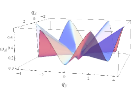
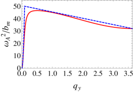
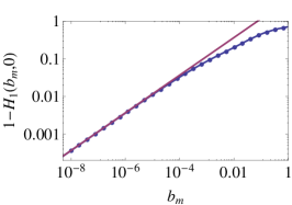
Figure 10: (a) Dispersion relation of the floppy mode taking $\mu_{m}=1,\kappa_{m}=0.0005,\lambda_{m}=0$, where the frequency $\omega_{A}$ is the square root of the lowest eigenvalue of $\mathbf{D}(\mu_{m},\kappa_{m}\lambda_{m})$. (b) The floppy mode branch of the eigenvalues of the dynamical matrix along the direction of $\pi/2$ (which is $q_{x}=0$) taking $\mu_{m}=1,\kappa_{m}=10^{-5},\lambda_{m}=0$. The red solid curve shows the actual eigenvalues calculated from the dynamical matrix numerically, and the blue dashed line shows the approximation we used in Eq. (52)  that $\omega_{A}^{2}=q_{y}^{2}/16$ if $q_{y}<Q_{s}$ and $\omega_{A}^{2}=16b_{m}g(q_{y})$ otherwise (only the $q_{y}>Q_{s}$ part is included in Eq. 52 because other contributions are much smaller). (c) Comparison between numerical (blue points connected by line) and the asymptotic form (59) (red line) of $1-H_{1}(b_{m},0)$.

It is straightforward to calculate the singular part of $\langle\mathbf{B}_{1}^{b}|\mathbf{H}(b_{m},0)|\mathbf{B}_{1}^{b}\rangle$ along symmetry directions of the floppy modes, which involves the integral

$$H_{2,\frac{\pi}{2},s}(b_{m},0)$$

$$= v_{0}\int_{1BZ,|q_{x}|\leq|q_{y}|/\sqrt{3}}\frac{d^{2}q}{(2\pi)^{2}}\frac{|\langle\mathbf{B}_{1,\mathbf{q}}^{b}|\nu_{f}\rangle|^{2}}{\frac{3}{16}q_{x}^{2}+b_{m}g(q_{y})}$$ (54)

where $v_{0}=\sqrt{3}/2$ is the area of the kagome lattice unit cell, and the condition $|q_{x}|\leq|q_{y}|/\sqrt{3}$ confines the integral to be around the floppy mode directions $\pi/2$ and $3\pi/2$ near which the expansion (52) is valid. The total contribution involves the singular part of all the isostatic directions

$$H_{2,s}=H_{2,\frac{\pi}{2},s}+H_{2,\frac{\pi}{6},s}+H_{2,\frac{5\pi}{6},s}.$$ (55)

All these terms exhibit similar behavior so we just discuss $H_{2,\frac{\pi}{2},s}$ for convenience. In Eq. (B.1), assuming $b_{m}\ll 1$, one can first integrate out $q_{x}$ using contour integrals, which gives

$$H_{2,\frac{\pi}{2},s}(b_{m},0) \simeq\frac{1}{(2\pi)^{2}/v_{0}}\int_{0}^{\frac{2\pi}{\sqrt{3}}}dq_{y}\frac{4\pi}{\sqrt{3}}\frac{|\langle\mathbf{B}_{1,\mathbf{q}}^{b}|\nu_{f}\rangle|^{2}}{\sqrt{b_{m}g(q_{y})}}$$

$$\sim b_{m}^{-1/2}$$ (56)

indicating a leading order divergence $b_{m}^{-1/2}$ of $H_{2}$ at small $\kappa_{m}$. A calculation including all terms in Eq. (55) yields

$$H_{2,s}(b_{m},0)\simeq\frac{\sqrt{A}}{2}b_{m}^{-1/2},$$ (57)

where

$$\frac{\sqrt{A}}{2}=20(1-\sqrt{2/3}).$$ (58)

From this we get

$$H_{1}(b_{m},0)\simeq 1-\frac{\sqrt{A}}{2}b_{m}^{1/2}$$ (59)

at small $\kappa_{m}$. Plugging this back into Eq. (43a), we arrive at the solution

$$\frac{\mu_{m}}{\mu}= \frac{(\Delta p)^{2}}{A(2p-1)\kappa/(\mu a^{2})}$$

$$\cdot\left[-1+\sqrt{1+\frac{A(2p-1)\kappa/(\mu a^{2})}{(\Delta p)^{2}}}\right]^{2}$$ (60)

where $\Delta p\equiv 1-\Delta p$ and this solution is asymptotically accurate for $\kappa\ll 1$ and $\Delta p\ll 1$.

B.2 Asymptotic solution near $p=p_{\textrm{b}}$

The rigidity threshold $p_{\textrm{b}}$ can be obtained by plugging $\mu_{m}=0$ into Eqs. (43a,43b,43c), which leads to

$$p_{\textrm{b}} \simeq 0.6920,$$

$$b_{m} \simeq 0.03788,$$

$$l_{m} \simeq 0.008032.$$ (61)

Following the calculation in Ref. Mao et al. (2011) we arrive at the asymptotic solution for $\mu_{m}$

$$\mu_{m}=\mu\Phi(\kappa/(\mu a^{2}))(p-p_{b})$$ (62)

where

$$\Phi(x)=\frac{c_{2}x}{c_{1}+x}$$ (63)

with

$$c_{1} \simeq 0.03802$$

$$c_{2} \simeq 4.697.$$ (64)

Appendix C Asymptotic solutions to EMT II equations

The self-consistency equation of the EMT II can be written as Das et al. (2007, 2012)

$$\frac{\mu_{m}}{\mu} =\frac{p-a^{*}}{1-a^{*}},$$

$$\frac{\kappa_{m}}{\kappa} =\frac{p^{2}-b^{*}}{1-b^{*}}$$ (65)

where the variables $a^{*}$ and $b^{*}$ correspond to the integrals we defined as

$$a^{*} =H_{1}$$

$$b^{*} =(\kappa_{m}/\mu_{m})H_{2}$$ (66)

as shown in Ref. Mao et al. (2011).

Using the asymptotic forms we obtained in Eqs. (57,59), we have

$$\frac{\mu_{m}}{\mu} =\frac{p-1+(\sqrt{A}/2)(\kappa_{m}/\mu_{m})^{1/2}}{(\sqrt{A}/2)(\kappa_{m}/\mu_{m})^{1/2}},$$ (67)

$$\frac{\kappa_{m}}{\kappa} =\frac{p^{2}-(\sqrt{A}/2)(\kappa_{m}/\mu_{m})^{1/2}}{1-(\sqrt{A}/2)(\kappa_{m}/\mu_{m})^{1/2}}.$$ (68)

Close to $p=1$, if we take $\kappa/\mu\ll 1$, then $(\sqrt{A}/2)(\kappa_{m}/\mu_{m})^{1/2}\ll 1$ and we have

$$\kappa_{m}/\kappa\simeq 1.$$ (69)

Plugging this back into Eq. (67) we get

$$\frac{\mu_{m}}{\mu} =\frac{p-1+(\sqrt{A}/2)(\kappa/\mu_{m})^{1/2}}{(\sqrt{A}/2)(\kappa/\mu_{m})^{1/2}}$$ (70)

which is a quadratic equation in $\mu_{m}^{1/2}$, and the solution to this leads to the same asymptotic solution as in Eqs. (B.1,15).

Next we discuss asymptotic behaviors near the rigidity threshold $p_{b,2}$ (the subscript $2$ is used to distinguish it from the threshold $p_{\textrm{b}}$ in EMT I). The value of $p_{b,2}$ in EMT II can be readily obtained from

$$0 =p-a^{*},$$

$$0 =p^{2}-b^{*},$$ (71)

along with the condition that $a^{*}+b^{*}=2d/z$, as discussed in the App. D of Ref. Mao et al. (2011). We then have

$$p_{b,2}=\frac{1}{2}\left(-1+\sqrt{1+\frac{8d}{z}}\right)\simeq 0.6180.$$ (72)

The EMT II self-consistency equations 65 can then be expanded at small

$$\Delta p=p-p_{b,2},$$ (73)

and this leads to

$$\mu_{m}=\mu\Phi_{2}\left(\kappa/(\mu a^{2})\right)(p-p_{b,2})$$ (74)

with

$$\Phi_{2}(x)=\frac{(2p_{b,2}+1)x}{p_{b,2}b_{b,2}+(1-p_{b,2})x}$$ (75)

This is in the same scaling form as in EMT I [Eqs. (LABEL:EQ:scaling-2) and (63)], apart from different constant factors.

References

- Chawla (1998) \BibitemOpen\bibfieldauthor K. Chawla, Fibrous Materials (Cambridge University Press, Cambridge, UK, 1998)\BibitemShutNoStop
- Gardel et al. (2004a) \BibitemOpen\bibfieldauthor M. L. Gardel, J. H. Shin, F. C. MacKintosh, L. Mahadevan, P. Matsudaira, and D. A. Weitz, \bibfieldjournal Science 304, 1301 (2004a)\BibitemShutNoStop
- Storm et al. (2005) \BibitemOpen\bibfieldauthor C. Storm, J. Pastore, F. MacKintosh, T. Lubensky, and P. Janmey, \bibfieldjournal Nature 435, 191 (2005)\BibitemShutNoStop
- Onck et al. (2005) \BibitemOpen\bibfieldauthor P. R. Onck, T. Koeman, T. van Dillen, and E. van der Giessen, \bibfieldjournal Phys. Rev. Lett. 95, 178102 (2005)\BibitemShutNoStop
- Kang et al. (2009) \BibitemOpen\bibfieldauthor H. Kang, Q. Wen, P. A. Janmey, J. X. Tang, E. Conti, and F. C. MacKintosh, \bibfieldjournal Journal of Physical Chemistry B 113, 3799 (2009)\BibitemShutNoStop
- Janmey et al. (2007) \BibitemOpen\bibfieldauthor P. A. Janmey, M. E. McCormick, S. Rammensee, J. L. Leight, P. C. Georges, and F. C. Mackintosh, \bibfieldjournal Nature Materials 6, 48 (2007)\BibitemShutNoStop
- Heussinger and Frey (2006) \BibitemOpen\bibfieldauthor C. Heussinger and E. Frey, \bibfieldjournal Phys. Rev. Lett. 97, 105501 (2006)\BibitemShutNoStop
- Heussinger et al. (2007) \BibitemOpen\bibfieldauthor C. Heussinger, B. Schaefer, and E. Frey, \bibfieldjournal Physical Review E 76, 031906 (2007)\BibitemShutNoStop
- Huisman et al. (2008) \BibitemOpen\bibfieldauthor E. M. Huisman, C. Storm, and G. T. Barkema, \bibfieldjournal Physical Review E 78, 051801 (2008)\BibitemShutNoStop
- Head et al. (2003a) \BibitemOpen\bibfieldauthor D. A. Head, A. J. Levine, and F. C. MacKintosh, \bibfieldjournal Phys. Rev. Lett. 91, 108102 (2003a)\BibitemShutNoStop
- Head et al. (2003b) \BibitemOpen\bibfieldauthor D. A. Head, A. J. Levine, and F. C. MacKintosh, \bibfieldjournal Phys. Rev. E 68, 061907 (2003b)\BibitemShutNoStop
- Gardel et al. (2004b) \BibitemOpen\bibfieldauthor M. L. Gardel, J. H. Shin, F. C. MacKintosh, L. Mahadevan, P. A. Matsudaira, and D. A. Weitz, \bibfieldjournal Physical Review Letters 93, 188102 (2004b)\BibitemShutNoStop
- Alberts et al. (2008) \BibitemOpen\bibfieldauthor B. Alberts, A. Johnson, J. Lewis, M. Raff, K. Roberts, and P. Walter, Molecular Biology of the Cell, 4th ed. (Garland, New York, 2008)\BibitemShutNoStop
- Elson (1988) \BibitemOpen\bibfieldauthor E. L. Elson, \bibfieldjournal Annu. Rev. Biophys. Biophys. Chem 17, 397 (1988)\BibitemShutNoStop
- Janmey et al. (1997) \BibitemOpen\bibfieldauthor P. Janmey, S. Hvidt, J. Lamb, and T. Stossel, \bibfieldjournal Nature 345, 89 (1997)\BibitemShutNoStop
- Kasza et al. (2007) \BibitemOpen\bibfieldauthor K. Kasza, A. Rowat, J. Liu, T. Angelini, C. Brangwynne, G. Koenderink, and D. Weitz, \bibfieldjournal Curr. Opin. Cell Biol. 19, 101 (2007)\BibitemShutNoStop
- Latva-Kokko et al. (2001) \BibitemOpen\bibfieldauthor M. Latva-Kokko, J. Mäkinen, and J. Timonen, \bibfieldjournal Phys. Rev. E 63, 046113 (2001)\BibitemShutNoStop
- Latva-Kokko and Timonen (2001) \BibitemOpen\bibfieldauthor M. Latva-Kokko and J. Timonen, \bibfieldjournal Phys. Rev. E 64, 066117 (2001)\BibitemShutNoStop
- Wilhelm and Frey (2003) \BibitemOpen\bibfieldauthor J. Wilhelm and E. Frey, \bibfieldjournal Phys. Rev. Lett. 91, 108103 (2003)\BibitemShutNoStop
- Soven (1969) \BibitemOpen\bibfieldauthor P. Soven, \bibfieldjournal Phys. Rev. 178, 1136 (1969)\BibitemShutNoStop
- Kirkpatrick et al. (1970) \BibitemOpen\bibfieldauthor S. Kirkpatrick, B. Velický, and H. Ehrenreich, \bibfieldjournal Phys. Rev. B 1, 3250 (1970)\BibitemShutNoStop
- Elliott et al. (1974) \BibitemOpen\bibfieldauthor R. J. Elliott, J. A. Krumhansl, and P. L. Leath, \bibfieldjournal Rev. Mod. Phys. 46, 465 (1974)\BibitemShutNoStop
- Das et al. (2007) \BibitemOpen\bibfieldauthor M. Das, F. C. MacKintosh, and A. J. Levine, \bibfieldjournal Phys. Rev. Lett. 99, 038101 (2007)\BibitemShutNoStop
- Broedersz et al. (2011) \BibitemOpen\bibfieldauthor C. P. Broedersz, X. M. Mao, T. C. Lubensky, and F. C. MacKintosh, \bibfieldjournal Nature Physics 7, 983 (2011)\BibitemShutNoStop
- Mao et al. (2011) \BibitemOpen\bibfieldauthor X. Mao, O. Stenull, and T. C. Lubensky, \bibfieldjournal http://arxiv.org/abs/1111.1751 (2011)\BibitemShutNoStop
- Das et al. (2012) \BibitemOpen\bibfieldauthor M. Das, D. A. Quint, and J. M. Schwarz, \bibfieldjournal PLoS One 7, e35939 (2012)\BibitemShutNoStop
- MacKintosh et al. (1995) \BibitemOpen\bibfieldauthor F. C. MacKintosh, J. Käs, and P. A. Janmey, \bibfieldjournal Phys. Rev. Lett. 75, 4425 (1995)\BibitemShutNoStop
- Peichocka et al. (2012) \BibitemOpen\bibfieldauthor I. Peichocka, K. Jansen, C. Broedersz, F. MacKintosh, and G. Koenderink, \bibfieldjournal http://arxiv.org/abs/1206.3894 (2012)\BibitemShutNoStop
- Marko and Siggia (1995) \BibitemOpen\bibfieldauthor J. Marko and E. Siggia, \bibfieldjournal Macromolecules 28, 8759 (1995)\BibitemShutNoStop
- Feng and Sen (1984) \BibitemOpen\bibfieldauthor S. Feng and P. N. Sen, \bibfieldjournal Phys. Rev. Lett. 52, 216 (1984)\BibitemShutNoStop
- Jacobs and Thorpe (1995) \BibitemOpen\bibfieldauthor D. J. Jacobs and M. F. Thorpe, \bibfieldjournal Phys. Rev. Lett. 75, 4051 (1995)\BibitemShutNoStop
- Huisman et al. (2010) \BibitemOpen\bibfieldauthor E. M. Huisman, C. Storm, and G. T. Barkema, \bibfieldjournal Physical Review E 82 , 061902 (2010)\BibitemShutNoStop
- Stenull (2011) \BibitemOpen\bibfieldauthor O. Stenull, T. C. Lubensky, \bibfieldjournal arXiv:1108.4328v1 [cond-mat.soft] (2011)\BibitemShutNoStop
- Broedersz et al. (2012) \BibitemOpen\bibfieldauthor C. P. Broedersz, M. Sheinman, and F. C. MacKintosh, \bibfieldjournal Physical Review Letters 108, 078102 (2012)\BibitemShutNoStop
- Maxwell (1864) \BibitemOpen\bibfieldauthor J. C. Maxwell, \bibfieldjournal Philosophical Magazine 27, 294 (1864)\BibitemShutNoStop
- Souslov et al. (2009) \BibitemOpen\bibfieldauthor A. Souslov, A. J. Liu, and T. C. Lubensky, \bibfieldjournal Phys. Rev. Lett. 103, 205503 (2009)\BibitemShutNoStop
- Sun et al. (2012) \BibitemOpen\bibfieldauthor K. Sun, A. Souslov, X. Mao, and T. C. Lubensky, \bibfieldjournal PNAS 109, 12369– (2012)\BibitemShutNoStop
- Calladine (1978) \BibitemOpen\bibfieldauthor C. Calladine, \bibfieldjournal International Journal of Solids and Structures 14, 161 (1978)\BibitemShutNoStop
- Gurtner and Durand (2009) \BibitemOpen\bibfieldauthor G. Gurtner and M. Durand, \bibfieldjournal Epl 87, 24001 (2009)\BibitemShutNoStop
- DiDonna and Lubensky (2005) \BibitemOpen\bibfieldauthor B. A. DiDonna and T. C. Lubensky, \bibfieldjournal Phys. Rev. E 72, 066619 (2005)\BibitemShutNoStop
- Huisman and Lubensky (2011) \BibitemOpen\bibfieldauthor E. M. Huisman and T. C. Lubensky, \bibfieldjournal Physical Review Letters 106, 088301 (2011)\BibitemShutNoStop
- Mao and Lubensky (2011) \BibitemOpen\bibfieldauthor X. Mao and T. C. Lubensky, \bibfieldjournal Phys. Rev. E 83, 011111 (2011)\BibitemShutNoStop