A new geometric approach to latent topic modeling and discovery

Abstract

A new geometrically-motivated algorithm for nonnegative matrix factorization is developed and applied to the discovery of latent “topics” for text and image “document” corpora. The algorithm is based on robustly finding and clustering extreme-points of empirical cross-document word-frequencies that correspond to novel “words” unique to each topic. In contrast to related approaches that are based on solving non-convex optimization problems using suboptimal approximations, locally-optimal methods, or heuristics, the new algorithm is convex, has polynomial complexity, and has competitive qualitative and quantitative performance compared to the current state-of-the-art approaches on synthetic and real-world datasets.

Index Terms—  Topic modeling, nonnegative matrix factorization (NMF), extreme points, subspace clustering.

1 Introduction

Topic modeling is a statistical tool for the automatic discovery and comprehension of latent thematic structure or topics, assumed to pervade a corpus of documents.

Suppose that we have a corpus of $M$ documents composed of words from a vocabulary of $W$ distinct words indexed by $w=1,\ldots,W$. In the classic “bags of words” modeling paradigm widely-used in Probabilistic Latent Semantic Analysis [1] and Latent Dirichlet Allocation (LDA) [2, 3], each document is modeled as being generated by $N$ independent and identically distributed (iid) drawings of words from an unknown $W\times 1$ document word-distribution vector. Each document word-distribution vector is itself modeled as an unknown probabilistic mixture of $K<\min(M,W)$ unknown $W\times 1$ latent topic word-distribution vectors that are shared among the $M$ documents in the corpus. The goal of topic modeling then is to estimate the latent topic word-distribution vectors and possibly the topic mixing weights for each document from the empirical word-frequency vectors of all documents. Topic modeling has also been applied to various types of data other than text, e.g., images, videos (with photometric and spatio-temporal feature-vectors interpreted as the words), genetic sequences, hyper-spectral images, voice, and music, for signal separation and blind deconvolution.

If $\beta$ denotes the unknown $W\times K$ topic-matrix whose columns are the $K$ latent topic word-distribution vectors and $\theta$ denotes the $K\times M$ weight-matrix whose $M$ columns are the mixing weights over $K$ topics for the $M$ documents, then each column of the $W\times M$ matrix $A=\beta\theta$ corresponds to a document word-distribution vector. Let $X$ denote the observed $W\times M$ words-by-documents matrix whose $M$ columns are the empirical word-frequency vectors of the $M$ documents when each document is generated by $N$ iid drawings of words from the corresponding column of the $A$ matrix. Then given only $X$ and $K$, the goal is to estimate the topic matrix $\beta$ and possibly the weight-matrix $\theta$. This can be formulated as a nonnegative matrix factorization (NMF) problem [4, 5, 6, 7] where the typical solution strategy is to minimize a cost function of the form

$$\|X-\beta\theta\|^{2} + \psi(\beta,\theta)$$ (1)

where the regularization term $\psi$ is introduced to enforce desirable properties in the solution such as uniqueness of the factorization, sparsity, etc. The joint optimization of (1) with respect to $(\beta,\theta)$ is, however, non-convex and necessitates the use of suboptimal strategies such as alternating minimization, greedy gradient descent, local search, approximations, and heuristics. These are also typically sensitive to small sample sizes (words per document) $N$ especially when $N\ll W$ because many words may not be sampled and $X$ may be far from $A$ in Euclidean distance. In LDA, the columns of $\beta$ and $\theta$ are modeled as iid random drawings from Dirichlet prior distributions. The resulting maximum aposteriori probability estimation of $(\beta,\theta)$, however, turns out to be a fairly complex non-convex problem. One then takes recourse to sub-optimal solutions based on variational Bayes approximations of the posterior distribution and other methods based on Gibbs sampling and expectation propagation.

In contrast to these approaches we adopt the non-negative matrix factorization framework and propose a new geometrically motivated algorithm that has competitive performance compared to the current state-of-the art and is free of heuristics and approximations.

2 A new geometric approach

A key ingredient of the new approach is the so-called “separability” assumption introduced in [5] to ensure the uniqueness of nonnegative matrix factorization. Applied to $\beta$ this means that each topic contains “novel” words which appear only in that topic – a property that has been found to hold in the estimates of topic matrices produced by several algorithms [8]. More precisely, A $W\times K$ topic matrix $\beta$ is separable if for each $k\in[1,K]$, there exists a row of $\beta$ that has a single non-zero entry which is in the $k$-th column. Figure 1 shows an example of a separable topic matrix with three topics. Words 1 and 2 are unique (novel) to topic 1, words 3, 4 to topic 2, and word 5 to topic 3.

Let $\mathcal{C}_{k}$ be the set of novel words of topic $k$ for $k\in[1,K]$ and let $\mathcal{C}_{0}$ be the remaining words in the vocabulary. Let $A_{w}$ and $\theta_{k}$ denote the $w$-th and $k$-th row-vectors of $A$ and $\theta$ respectively. Observe that all the row-vectors of $A$ that correspond to the novel words of the same topic are just different scaled versions of the same $\theta$ row-vector: for each $w\in\mathcal{C}_{k}$, $A_{w}=\beta_{wk}\theta_{k}$. Thus if $\widetilde{A}$, $\widetilde{\beta}$, and $\widetilde{\theta}$ denote the row-normalized versions (i.e., unit row sums) of $A$, $\beta$, and $\theta$ respectively then $\widetilde{A}=\widetilde{\beta}\widetilde{\theta}$ and for all $w\in\mathcal{C}_{k},\widetilde{A}_{w}=\widetilde{\theta}_{k}$ (e.g., in Fig. 1, $\widetilde{A}_{1}=\widetilde{A}_{2}=\widetilde{\theta}_{1}$ and $\widetilde{A}_{3}=\widetilde{A}_{4}=\widetilde{\theta}_{2}$), and for all $w\in\mathcal{C}_{0}$, $\widetilde{A}_{w}$ lives in the convex hull of $\widetilde{\theta}_{k}$’s (in Fig. 1, $\widetilde{A}_{6}$ is in the convex hull of $\widetilde{\theta}_{1},\widetilde{\theta}_{2},\widetilde{\theta}_{3}$).

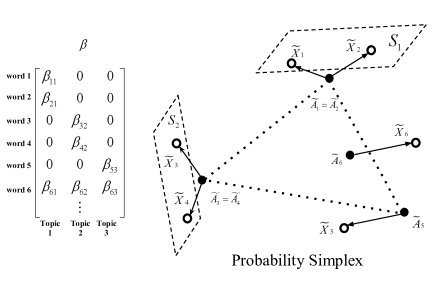
Fig. 1: A separable topic matrix and the underlying geometric structure. Solid circles represent rows of $\widetilde{A}$, empty circles represent rows of $\widetilde{X}$.

This geometric viewpoint reveals how to extract the topic matrix $\beta$ from $A$: (1) Row-normalize $A$ to $\widetilde{A}$. (2) Find extreme points of $\widetilde{A}$’s row-vectors. (3) Cluster the row-vectors of $\widetilde{A}$ that correspond to the same extreme point into the same group. There will be $K$ disjoint groups and each group will correspond to the novel words of the same topic. (4) Express the remaining row-vectors of $\widetilde{A}$ as convex combinations of the extreme points. This gives us $\widetilde{\beta}$ (5) Finally, renormalize $\widetilde{\beta}$ to obtain $\beta$.

The reality, however, is that we only have access to $X$, not $A$. The above algorithm when applied to $X$ would work well if $X$ is close to $A$ which would happen if $N$ is large. When $N$ is small, two problems arise: (i) Points corresponding to novel words of the same topic may become multiple extreme points and may be far from each other (e.g., $\widetilde{X}_{1},\widetilde{X}_{2}$ and $\widetilde{X}_{3},\widetilde{X}_{4}$ in Fig. 1). (ii) Points in the convex hull may also become “outlier” extreme points (e.g., $\widetilde{X}_{6}$ in Fig. 1).

As a step towards overcoming these difficulties we observe that in practice, the unique words of any topic only occur in a few documents. This implies that the rows of $\theta$ are sparse and that the row-vectors of $\widetilde{X}$ corresponding to the novel words of the same topic are likely to form a low-dimensional subspace (e.g., $S_{1},S_{2}$ in Fig. 1) since their supports are subsets of the supports of the same row-vector of $\theta$. If we make the further assumption that for any pair of distinct topics there are several documents in which their novel words do not co-occur then the row subspaces of $\widetilde{X}$ corresponding to the novel words any two distinct topics are likely to be significantly disjoint (although they might share a common low-dimensional subspace). Finally, the row-vectors of $\widetilde{X}$ corresponding to non-novel words are unlikely to be close to the row subspaces of $\widetilde{X}$ corresponding to the novel words any one topic (e.g., $\widetilde{X}_{6}$ in Fig. 1). These observations and assumptions motivate the revised $5$-step Algorithm 1 for extracting $\beta$ from $X$.

Algorithm 1 Topic Discovery

1:$W\times M$ word-document matrix $X$; # topics $K$.

2:Estimate $\widehat{\beta}$ of $W\times K$ topic matrix $\beta$.

3:Row-normalize $X$ to get $\widetilde{X}$. Let $N_{w}:=\sum_{d=1}^{M}{X}_{wd}$.

4:Apply Algorithm 2 to rows of $\widetilde{X}$ to obtain a subset of rows $\mathcal{E}$ that correspond to candidate novel words. Let $\widehat{\mathcal{C}}_{0}$ be the remaining row indices.

5:Apply the sparse subspace clustering algorithm of [9, 10] to $\mathcal{E}$ with parameters $\lambda_{1},\gamma$ to obtain $K$ clusters $\{\widehat{\mathcal{C}}_{k}\}_{k=1}^{K}$ of novel words and cluster $\mathcal{C}_{out}$ of outlier words. Rearrange the rows of $\widetilde{X}$ indexed by $\widehat{\mathcal{C}_{k}}$ into a matrix $Y_{k}$.

6:For each $w\in\widehat{\mathcal{C}}_{0}\bigcup\mathcal{C}_{out}$, solve

$$\min\limits_{\{{b}_{wl}\in\mathbb{R}_{+}^{|\widehat{\mathcal{C}}_{l}|}\}_{l=1}^{K}}\|\widetilde{X}_{w}-\sum_{l=1}^{K}b_{wl}Y_{l}\|_{2}^{2}+\lambda_{2}\sum_{l=1}^{K}\|b_{wl}\|_{\infty}$$

for some $\lambda_{2}\geq 0$. Let $\{b_{wl}^{*}\}_{l=1}^{K}$ be the optimal solution.

7:For $w=1,\ldots,W$, $k=1,\ldots,K$, set

$$\widehat{\beta}_{wk}=\left\{\begin{array}[]{lcl}N_{w}{\mathbf{1}}(w\in\widehat{\mathcal{C}}_{k})&\mbox{for}&w\in\bigcup_{l=1}^{K}\widehat{\mathcal{C}}_{l}\\ N_{w}\|b_{wk}^{*}\|_{1}&\mbox{for}&w\in\widehat{\mathcal{C}}_{0}\bigcup\mathcal{C}_{out}\end{array}\right.$$

and normalize each column of $\widehat{\beta}$ to be column stochastic.

Algorithm 2 Find candidate novel words

1:Set of $1\times M$ probability row-vectors $\widetilde{x}_{1},\ldots,\widetilde{x}_{W}$; Number of projections $P$; Tolerance $\delta$.

2:Set $\mathcal{E}$ of candidate novel row-vectors.

3:Set $\mathcal{E}=\emptyset$.

4:Generate row-vector $d\sim$ Uniform(unit-sphere in $\mathbb{R}^{M})$.

5:$i_{max}:=\arg\max_{i}\widetilde{x}_{i}d^{T}$, $i_{min}:=\arg\min_{i}\widetilde{x}_{i}d^{T}$.

6:$\mathcal{E}\leftarrow\mathcal{E}\bigcup\{x_{i}:\|x_{i}-x_{i_{max}}\|_{1}\leq\delta\mbox{ or }\|x_{i}-x_{i_{min}}\|_{1}\leq\delta\}$.

7:Repeat steps $2$ through $4$, $P$ times.

Step (2) of Algorithm 1 finds rows of $\tilde{X}$ many of which are likely to correspond to the novel words of topics and some to outliers (non-novel words). This step uses Algorithm 2 which is a linear-complexity procedure for finding, with high probability, extreme points and points close to them (the candidate novel words of topics) using a small number $P$ of random projections. Step (3) uses the state-of-the-art sparse subspace clustering algorithm from [9, 10] to identify $K$ clusters of novel words, one for each topic, and an additional cluster containing the outliers (non-novel words). Step (4) expresses rows of $\widetilde{X}$ corresponding to non-novel words as convex combinations of these $K$ groups of rows and step (5) estimates the entries in the topic matrix and normalizes it to make it column-stochastic. In many applications, non-novel words occur in only a few topics. The group-sparsity penalty $\lambda_{2}\sum_{l=1}^{K}\|b_{wl}\|_{\infty}$ proposed in [11] is used in step (4) of Algorithm 1 to favor solutions where the row vectors of non-novel words are convex combinations of as few groups of novel words as possible. Our proposed algorithm runs in polynomial-time in $W$, $M$, and $K$ and all the optimization problems involved are convex.

3 Experimental results

3.1 Synthetic Dataset

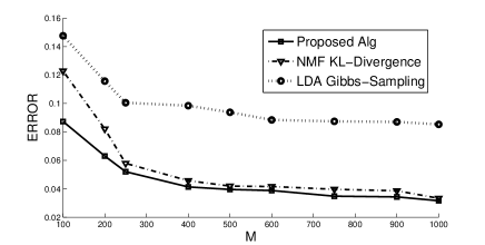
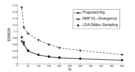
Fig. 2: Error of estimated topic matrix in Frobenius norm. Upper: $W=500,\rho=0.2,N=50,K=5$; Lower: $W=500,\rho=0.2,K=10,M=500$.

In this section, we validate our algorithm on some synthetic examples. We generate a $W\times K$ separable topic matrix $\beta$ with $W_{1}/K>1$ novel words per topic as follows: first, iid $1\times K$ rows-vectors corresponding to non-novel words are generated uniformly on the probability simplex. Then, $W_{1}$ iid $\mathrm{Uniform}[0,1]$ values are generated for the nonzero entries in the rows of novel words. The resulting matrix is then column-normalized to get one realization of $\beta$. Let $\rho:=W_{1}/W$. Next, $M$ iid $K\times 1$ column-vectors are generated for the $\theta$ matrix according to a Dirichlet prior $c\prod\limits_{i=1}^{K}\theta_{i}^{\alpha_{i}-1}$. Following [12], we set $\alpha_{i}=0.1$ for all $i$. Finally, we obtain $X$ by generating $N$ iid words for each document.

For different settings of $W$, $\rho$, $K$, $M$ and $N$, we calculate the error of the estimated topic matrix $\widehat{\beta}$ as $\|\widehat{\beta}-\beta\|_{F}$. For each setting we average the error over $50$ random samples. In sparse subspace clustering the value of $\lambda_{1}$ is set as in [10] (it depends on the size of the candidate set) and the value of $\gamma$ as in [9] (it depends on the values of $N,M$). In Step 4 of Algorithm 1, we set $\lambda_{2}=0.01$ for all settings.

We compare our algorithm against the LDA algorithm [2] and a state-of-art NMF-based algorithm [13]. This NMF algorithm is chosen because it compensates for the type of noise we use in our topic model. Our LDA algorithm uses Gibbs sampling for inferencing. Figure 2 depicts the estimation error as a function of the number of documents $M$ (top) and the number of words/document $N$ (bottom). Evidently, our algorithm is uniformly better than comparable techniques. Specifically, while NMF has similar error as our algorithm for large $M$ it performs relatively poorly as a function of $N$. On the other hand LDA has similar error performance as ours for large $N$ but performs poorly as a function of $M$. Note that both of these algorithms have comparably high error rates for small $M$ and $N$.

3.2 Swimmer Image Dataset

(a)

(b)

(c)

Fig. 3: (a) Example “clean” images (cols. of $A$) in Swimmer dataset; (b) Corresponding images with sampling “noise” (cols. of $X$); (c) Examples of ideal topics (cols. of $\beta$).

Pos.	LA 1	LA 2	LA 3	LA 4	RA 1	RA 2	RA 3	RA 4	LL 1	LL 2	LL 3	LL 4	RL 1	RL 2	RL 3	RL 4
a)
b)
c)

Fig. 4: Topics estimated for noisy swimmer dataset by a) proposed algorithm, b) LDA inference using code in [12], c) NMF algorithm using code in [13]. Topics closest to the 16 ideal (ground truth) topics LA1, LA2, etc., are shown. LDA misses $5$ and NMF misses $6$ of the ground truth topics while our algorithm recovers all $16$ and our topic estimates look less noisy.

a)
b)

Fig. 5: Topic errors for (a) LDA algorithm [12] and (b) NMF algorithm [13] on the Swimmer dataset. Figure depicts topics that are extracted by LDA and NMF but are not close to any “ground truth” topic. The ground truth topics correspond to 16 different positions of left/right arms and legs.

In this section we apply our algorithm to the synthetic swimmer image dataset introduced in [5]. There are $M=256$ binary images each of $W=32\times 32=1024$ pixels. Each image represents a swimmer composed of four limbs, each of which can be in one of $4$ distinct positions, and a torso.

We interpret pixel positions $(i,j),1\leq i,j\leq 32$ as words in a dictionary. Documents are images, where an image is interpreted as a collection of pixel positions with non-zero values. Since each of the four limbs can independently take one of four positions, it turns out that the topic matrix $\beta$ satisfies the separability assumption with $K=16$ “ground truth” topics that correspond to $16$ single limb positions. Following the setting of [13], we set body pixel values to 10 and background pixel values to 1. We then take each “clean” image, suitably normalized, as an underlying distribution across pixels and generate a “noisy” document of $N=200$ iid “words” according to the topic model. Examples are shown in Fig. 3. We then apply our algorithm to the “noisy” dataset. We again compare our algorithm against LDA and the NMF algorithm from [13]. Results are shown in Figures 4 and 5. Values of tuning parameters $\lambda_{1},\gamma$, and $\lambda_{2}$ are set as in Sec. 3.1. Specifically, $\lambda_{1}=0.1,\lambda_{2}=0.01$ for the results in Figs. 4 and 5.

This dataset is a good validation test for different algorithms since the ground truth topics are known and are unique. As we see in Fig. 5, both LDA and NMF produce topics that do not correspond to any pure left/right arm/leg positions. Indeed, many estimated topics are composed of multiple limbs. Nevertheless, no such errors are realized in our algorithm and our topic-estimates are closer to the ground truth images.

3.3 Text Corpora

“chips”	“vision”	“networks”	“learning”
chip	visual	network	learning
circuit	cells	routing	training
analog	ocular	system	error
current	cortical	delay	SVM
gate	activity	load	model

“election”	“law”	“market”	“game”
state	case	market	game
politics	law	executive	play
election	lawyer	industry	team
campaign	charge	sell	run
vote	court	business	season

Table 1: Most frequent words in examples of estimated topics. Upper: NIPS, with $K=40$ topics; Lower: NY Times, with $K=20$ topics

In this section, we apply our algorithm on two different text corpora, namely, the NIPS dataset [14] and the New York (NY) Times dataset [15]. In the NIPS dataset, there are $M=2484$ documents with $W=14036$ words in the vocabulary. There are, on average, $N\approx 900$ words in each document. In the NY Times dataset, $M=3000$, $W=9340$, and $N\approx 270$. The vocabulary is obtained by deleting a standard “stop” word list used in computational linguistics, including numbers, individual characters, and some common English words such as “the”. Words that occur less than $5$ times in the dataset and the words that occur in less than $5$ documents are removed from the vocabulary as well. The tuning parameters $\lambda_{1},\gamma,$ and $\lambda_{2}$ are set in the same way as in Sec. 3.1 (specifically, $\lambda_{1}=0.1$ and $\lambda_{2}=0.1$).

Table 1 depicts typical topics extracted by our algorithm. For each topic we show its most frequent words, listed in descending order of estimated probability. Although there is no “ground truth” to compare with, the most frequent words in the estimated topics do form recognizable themes. For example, in the NIPS dataset, the set of (most frequent) words “chip”, “circuit”, etc., can be annotated as “IC Design”; The words “visual”, “cells”, etc., can be labeled as “human visual system”. As a point of comparison, we also experimented with related convex programming algorithms [8, 7] that have recently appeared in the literature. We found that they fail to produce meaningful results for these datasets.

References

- [1] T. Hofmann, “Probabilistic latent semantic analysis,” in Uncertainty in Artificial Intelligence, San Francisco, CA, 1999, pp. 289–296, Morgan Kaufmann Publishers.
- [2] D. M. Blei, A. Y. Ng, and M. I. Jordan, “Latent dirichlet allocation,” J. Mach. Learn. Res., vol. 3, pp. 993–1022, Mar. 2003.
- [3] D. M. Blei, “Probabilistic topic models,” Commun. ACM, vol. 55, no. 4, pp. 77–84, Apr. 2012.
- [4] D. D. Lee ans H. S. Seung, “Learning the parts of objects by non-negative matrix factorization,” Nature, vol. 401, no. 6755, pp. 788–791, Oct. 1999.
- [5] D. Donoho and V. Stodden, “When does non-negative matrix factorization give a correct decomposition into parts?,” in Advances in Neural Information Processing Systems 16, Cambridge, MA, 2004, MIT Press.
- [6] A. Cichocki, R. Zdunek, A. H. Phan, and S. Amari, Nonnegative matrix and tensor factorizations: applications to exploratory multi-way data analysis and blind source separation, Wiley, 2009.
- [7] B. Recht, C. Re, J. Tropp, and V. Bittorf, “Factoring nonnegative matrices with linear programs,” in Advances in Neural Information Processing Systems 25, 2012, pp. 1223–1231.
- [8] S. Arora, R. Ge, and A. Moitra, “Learning topic models – going beyond SVD,” arXiv:1204.1956v2 [cs.LG], 2012.
- [9] M. Soltanolkotabi, and E. J. Candes, “A geometric analysis of subspace clustering with outliers,” ArXiv e-prints, Dec. 2011.
- [10] E. Elhamifar and R. Vidal, “Sparse subspace clustering: algorithm, theory, and applications,” IEEE Transactions on Pattern Analysis and Machine Intelligence, 2012.
- [11] E. Esser, M. Moller, S. Osher, G. Sapiro, and J. Xin, “A convex model for nonnegative matrix factorization and dimensionality reduction on physical space,” IEEE Trans. Image Processing, vol. 21, pp. 3239–3252, Jul. 2012.
- [12] T. Griffiths and M. Steyvers, “Finding scientific topics,” in Proceedings of the National Academy of Sciences, 2004, vol. 101, pp. 5228–5235.
- [13] V. Y. F. Tan and C. Févotte, “Automatic relevance determination in nonnegative matrix factorization with the beta-divergence,” IEEE Transactions on Pattern Analysis and Machine Intelligence, in press.
- [14] A. Globerson, G. Chechik, F. Pereira, and N. Tishby, “Euclidean embedding of co-occurrence data,” The Journal of Machine Learning Research, vol. 8, pp. 2265–2295, 2007.
- [15] A. Chaney and D. M. Blei, “Visualizing topic models,” in International AAAI Conference on Weblogs and Social Media, 2012.