The Analyticity Breakdown for Frenkel-Kontorova Models in Quasi-periodic Media: Numerical Explorations
Abstract.
We study numerically the “analyticity breakdown” transition in 1-dimensional quasi-periodic media. This transition corresponds physically to the transition between pinned down and sliding ground states. Mathematically, it corresponds to the solutions of a functional equation losing their analyticity properties.
We implemented some recent numerical algorithms that are efficient and backed up by rigorous results so that we can compute with confidence even close to the breakdown.
We have uncovered several phenomena that we believe deserve a theoretical explanation: A) The transition happens in a smooth surface. B) There are scaling relations near breakdown. C) The scaling near breakdown is very anisotropic. Derivatives in different directions blow up at different rates.
Similar phenomena seem to happen in other KAM problems.
Key words and phrases:
Quasi-periodic solutions, quasi-crystals, hull functions, KAM theory2000 Mathematics Subject Classification:
70K43, 52C23, 37A60, 37J40, 82B201. Introduction
In this paper we present detailed numerical results on the analyticity breakdown transition in models of one-dimensional quasi-periodic media. This analyticity breakdown transition is widely accepted to correspond to the transition between pinned down and sliding ground states. Hence, the position of the transition affects the properties of the material described by the models. For the physical motivation of the theory see Section 2 and [AA80, vE99].
From the mathematical point of view, the problem is to study the analyticity properties of the solution of a functional equation depending on parameters (the function is the hull function parameterizing a ground state and the functional equation is the expression that the system is in equilibrium). It is expected that, for some parameter values, the solution is analytic but that, as we move parameters, the domain of analyticity decreases and eventually disappears. See Section 2 for a more precise description of the problem.
The phenomenon of analyticity breakdown is very similar to the widely studied phenomena of breakdown of KAM tori in mechanics. Indeed, the problem of analyticity breakdown in periodic media is completely equivalent to the breakdown of KAM circles in two dimensional twist mappings. In the case of quasi-periodic media considered here, the problem does not seem to have an easy dynamical representation and the treatment of the functional equations describing the equilibria for KAM theory is very different from the Hamiltonian counterpart because, besides the lack of a dynamical interpretation, the system has an extra frequency. The KAM theory for the equilibrium equation in quasi-periodic media has been obtained recently in [SdlL12a, SdlL12b].
The KAM theory in [SdlL12a, SdlL12b] is very different from the regular KAM theory for two reasons: one is that the models do not admit an easy dynamical interpretation and a second reason is because the quasi-periodicity of the substratum introduces the an extra variable. This extra frequency has very drastic effects, which are not just mathematical artifacts. For instance, there are counterexamples to some standard predictions of the Aubry-Mather theory which describes the ground states in periodic media [LS03]. In the periodic case, when Aubry-Mather theory applies, the analyticity breakdown transition could be described as saying that the smooth tori break up into Cantori (see [Per79]). In the case of quasi-periodic media, we are not sure of what could take the place of the Aubry-Mather theory after the breakdown of KAM theory. This is a question that deserves further study, but which we are not considering in this paper.
Nevertheless, we expect that some of the phenomena studied in detail here, notably the anisotropic regularity at breakdown happen also in other KAM problems involving two-dimensional functions. Indications to that effect have already been found qualitatively [Tom96, HS99, CFL04], but in this paper we can obtain rather quantitative aspects of the phenomenon.
Since the main goal is to compute accurately functions as close as possible to their breakdown, it is clear that the numerics are going to be delicate and that it is very important to have criteria that allows to be confident that the computed solutions are correct. We note that the experience shows that close to the breakdown, the truncated equations admit many spurious solutions that do not correspond to truncations of true solutions of the equations [vEF02, GvE05].
In this paper we have implemented the algorithms suggested in [SdlL12a]. The main results of [SdlL12a] are based on a Newton method which is very efficient (see Section 3.4). If the function is discretized using Fourier coefficients, the Algorithm 3.2 gives quadratic convergence but requires only storage and arithmetic operations. Note that, even if we obtain the Newton-like quadratic convergence a step does not require to store (and much less to invert) an matrix.
Furthermore, the main result of [SdlL12a] is a result in a posteriori format. It asserts that, if we have a function which solves approximately the invariance equation (e.g. a numerical solution of the equation, where the error of truncation and round off is small) and that satisfy some easy to verify non-degeneracy assumptions corresponds to a true solution of the problem. Hence, by computing with a truncation, estimating the truncation error by changing the degree of the truncation and monitoring the non-degeneracy conditions, we may be reasonably confident that we have obtained a true solution.
Of course, a numerical implementation requires many more details than a mathematical algorithm and one has to discuss implementation issues such as data structures used, choice of iteration steps, order of truncation, etc. These considerations are undertaken in Section 4. The results are presented in Section 4.1 and the conclusions are presented in Section 5. We anticipate that the conclusions are A) The breakdown happens in a smooth surface, B) There are scaling relations. Sobolev norms of the function blow up as a power of the distance to the critical surface. C) The breakdown is extremely anisotropic.
Of course, A) and B) have been observed many times in phase transitions and are one of the predictions of renormalization group theory but C) seems somewhat unexpected. There have been visual observations indicating that the tori near breakdown look “filamented”. We think that there are reasons to expect that this phenomena will happen in other KAM problems involving several variables and we hope to come to that problem. In this paper, we will just present some numerical observations in a class of models.
2. The problem of analyticity breakdown
The simplest way to motivate the models studied here is to consider the problem of deposition of a material over a one-dimensional quasi-periodic substratum.
If represents the position of the particle of the deposited material, the state of the system is given by the configuration , which is sequence giving the position of all the deposited particles. Note that will be a real variable.
The Physics of the problem is obtained by assigning an formal energy to the configurations [Rue69, Isr79, Mat09]. This formal energy is obtained as a formal sum of the energies associated to every finite set of particles. Hopefully, most of the terms will be zero or decrease very fast with the diameter. Nevertheless, due to the translation invariance one does not hope that the sum of the energies converges.
The main example considered in this paper will be the quasi-periodic Frenkel-Kontorova model given by:
| (2.1) |
where and is a sufficiently irrational vector.
The term represents the interaction between nearest neighbors and the term represents the interaction with the substratum at the position . Note that this function is quasi-periodic as a reflection of the fact that the substratum is quasi-periodic. The classical Frenkel-Kontorova model [FK39] considered the case of periodic potentials with .
Other physical interpretations of the model are possible, for example, the classical [FK39] introduced the Frenkel-Kontorova model to describe the motion of planar dislocations in a crystal.
2.1. Some standard definitions
A configuration is in equilibrium when
| (2.2) |
Note that, even if the sum in (2.1) is a formal sum, the equilibrium equations (2.3) are very well defined.
A configuration is a ground state when
| (2.4) |
for all that vanish at all but a finite number of indices. Note that the left hand side of (2.4) can be given a good interpretation in the model (2.1) because the two formal sums only differ in a a finite number of sites.
A configuration is given by a hull function when we can find and such that
| (2.5) |
2.2. Equilibrium equations for hull functions. Formulation of our problem
Substituting (2.5) into (2.2), we obtain that an equilibrium configuration is given by a hull function if and only if
| (2.6) |
If is dense on (which is well known to happen if and only if for , [KH95]), for a continuous we obtain that (2.6) is equivalent to
| (2.7) |
Of course, it could well happen that there are discontinuous hull functions, but we are interested in studying precisely the existence of continuous – indeed analytic – functions.
Hence, (2.7) will be the centerpiece of our attention. We will fix satisfying good number theoretical properties, assume that depends on parameters and study numerically the set of parameters for which (2.7) has an analytic solution. We will pay special attention to the behavior of these solutions near the boundary of existence.
We note that the existence of a continuous solution of (2.7) implies that there is a continuous family of equilibrium configurations. On can note that for any , given by
| (2.8) |
is also a solution of (2.7). Hence, the configuration corresponding to it according to (2.5) is also an equilibrium configuration. The fact that we obtain a continuous family of configurations which are equilibria indicates that there is no energetic impediment to the solutions making small transitions and sliding. Hence one expects that the solutions can be modified easily. In contrast, if the set of equilibrium configurations is discontinuous, there may be an energetic barrier (the Peierls-Nabarro barrier) to perform jumps from a configuration to the nearest one and the solutions are pinned down.
Notice that corresponds to choosing a different origin of coordinates to the internal phase of the problem. This can be considered as a gauge symmetry of the problem. The Ward identities associated to this gauge symmetry play an important role in the study in [dlL08, CdlL10b, SdlL12a, SdlL12b] and also in our numerical treatment.
3. Mathematical results
3.1. An overview of the rigorous results
In the periodic case (), the problem of existence of continuous hull functions satisfying (2.7) is equivalent to the problem of existence of rotational invariant circles for a twist mapping [ALD83]. In the periodic case, there are several well developed mathematical theories which can lead to an understanding of the problem.
- •
- •
- •
In the periodic case, there are a number of numerical methods to study the breakdown. The appendix A of [CdlL10b] contains a comparative summary of the literature and compares the methods.
The KAM theory is perturbative but produces analytic solutions of (2.7) when the frequency satisfies some number theoretic properties (called “Diophantine”). Aubry-Mather theory is non-perturbative and it does not require any number theoretic properties of the function. On the other hand, the solutions of (2.7) may be discontinuous. The renormalization theory has as an aim to describe a subset of the boundary of analyticity. It was originally developed based on non-rigorous arguments supported by very careful numerics [Mac93], but by now there are quite a number of rigorous results (some of them proved by computer-assisted proofs).
In the quasi-periodic case considered here, the situation is very different. The Aubry-Mather theory seems somewhat problematic due to the examples in [LS03] (but there are some topological results in [GGP06]). To the best of our knowledge, there is no renormalization group theory for general quasi-periodic FK models (see, however [MO00]). There has been a recent development of a KAM theory in [SdlL12a, SdlL12b] which will be the basis of our work.
3.2. A posteriori results
The main result of [SdlL12a] is formulated in an a-posteriori format standard in numerical analysis.
We define the operator acting on hull functions by:
| (3.1) |
So that (2.7), the equilibrium equation for hull functions can be concisely expressed as
| (3.2) |
The main result of [SdlL12a] says (omitting some mathematical assumptions on regularity, definition of norms and number theoretic properties of ) that if we can find a function that satisfies approximately the equation (in some norm) and satisfies some non-degeneracy conditions, we can find a true solution and bound the distance from the true solution to the original guess (measured in another norm) by a constant times the size of the residual of the initial approximate solution.
Prototype Theorem 3.1.
Assume that we can find a function . such that
then, if
there exists a true solution of . and
Furthermore, the solution is the only solution (up to the gauge transformations associated to the change of origin in (2.8))
In the above, are rather explicit condition numbers. and is also an explicit function. Note that, as customary in KAM theory, there may be a loss of regularity and that the norm in which we measure the error may be different than the norm in which we reach the conclusions. In [SdlL12a], one can find results where the norms are norms in spaces of analytic functions and also results for Sobolev norms.
In applications, the approximate solution will be the product of a numerical calculation. It is important that in view of the above result, that to be confident that the approximate solution corresponds to a true solution, we do not need to study the algorithm used to produce it. We just need to verify that the condition numbers are reasonable and that the numerical error is small compared to them.
As we will see, the method of proof in [SdlL12a] is based on a rapidly convergent iterative method which is explicitly described. This method leads to an efficient algorithm (See Section 3.4, which we have implemented in Section 4 and which is the basis of our results. It is also important that the method leads to a numerically accesible criteria for breakdown, which we discuss in Section 3.3.
3.3. A numerically accessible criterion for breakdown of analyticity
In [CdlL10b], it was shown in great generality that, when one has an a posteriori result of the form Prototype 3.1 working for Sobolev and analytic spaces, one can get several results automatically.
Bootstrap of regularity All the solutions which are in a Sobolev space of order are analytic.
The critical value depends only on the number theoretic properties of .
Criterion for breakdown of analyticity If we consider a family depending on parameters, and obtain a family of approximate solutions with bounded non-degeneracy conditions, the parameters approach the boundary if and only if Sobolev norms of high enough order go to infinity.
Hence, it is clear how one should proceed. Implement the algorithm described in Section 3.4, run it monitoring the condition numbers (so that we are sure that we are not considering any spurious solutions) and the Sobolev norms. If the Sobolev norms blow up dramatically and nothing else happens, we are approaching the breakdown. Since the algorithm gives the Fourier coefficients of the hull function, the computation of the Sobolev norm is rather straightforward.
3.4. An efficient algorithm for a Newton method
The proof of [SdlL12a] is based on a Newton-like method that given an approximate solution produces a much more accurate one. The error after the correction is, roughly, the square of the error before the correction, but there is a loss of regularity. It is well known in the Nash-Moser hard implicit function theorems that these methods still lead to convergence.
The algorithm in [SdlL12a], which we detail below, is obtained taking advantage of several identities satisfied by (2.7) that come from its variational character and the gauge symmetry (2.8).
These identities reduce the Newton step to a sequence of elementary operations on functions (composing, taking derivatives, multiplying, solving difference equations with constant coefficients). A remarkable feature is that all of these operations are diagonal either in a discretization in Fourier terms or in a discretization based on points on a grid. Of course, the Fast Fourier Transform allows to pass from one discretization to another in a easy way.
The upshot is that if we discretize the function in terms of Fourier coefficients and the values at points in a grid, a Newton-like step requires storage and operations.
In practice, the constants in front of the asymptotics are moderate, since there are very optimized implementations of FFT for almost any architecture. As we will see, it is quite possible to use in a common desktop.
For the sake of completeness, we include verbatim the algorithm from [SdlL12a].
The algorithm of [SdlL12a] is actually slightly more general instead of (3.2) it consideres the equation
| (3.3) |
where , and both and are the unknowns.
The equation (3.3) allows to consider also also forces that do not come from a potential. Nevertheless, it is shown in [SdlL12a] that when the forces come from a potential, any solution of (3.3) satisfies and, hence gives a solution of (3.2).
As we will see, the algorithm consists of steps which are all elementary manipulations of functions (derivatives, multiplications, compositions) as well as solving the so called cohomology equations. That is, given periodic of period and with , find also periodic with period and with average such that
| (3.4) |
where .
Note that (3.4) can be solved very efficietly using Fourier coefficients and that it is equivalent to the equation for Fourier coefficients
The factor in parenthesis in the LHS vanishes for , and the equation for is overdetermined. It does not have a solution if , but if any is a solution, we choose the solution with . If is irrational, the term in parenthesis does not vanish for and, if it is Diophantine, we have lower bounds for it that lead to estimates for the solutions of the cohomology equation [Rüs75, Rüs76]. These estimates are used in [SdlL12a] to prove convergence of the algorithm, but in this paper, we will not discuss estimates.
Algorithm 3.2.
Given with and for and any irrational vector , we will perform the following calculations (where denotes the average)
-
1)
Let .
In Fourier components .
-
2)
We calculate .
-
3)
Calculate
-
4)
Calculate .
In Fourier components .
-
5)
Let .
-
6)
Choose .
-
7)
Denote .
-
8)
Solve the cohomology equation (3.4) for with zero average. That is, .
-
9)
Take
-
10)
Calculate .
-
11)
Solve the cohomology equation for . That is, where .
-
12)
We obtain .
-
13)
The new improved solution is , .
4. Numerical Implementation
The most computationally expensive steps in Algorithm 3.2 are diagonal in either real space or in frequency space, so we use the Fast Fourier Transform multiple times in each application of the Newton step. We use Matlab, and typically Fourier modes, so a discretization for is a complex-double. All non-degeneracy conditions are satisfied if the norm of the error is small enough, so we monitor the error throughout.
To implement the algorithm, we compute the error of an initial guess, then perform the Newton step to improve the guess, and then compute the new error for the improvement. If the new error is not below a threshold, the Newton step is performed again and the process repeats. If the new error is below the threshold, we conclude a torus exists nearby and we increase the parameter values. If the Newton step fails to bring the error below the threshold (after some number of attempts) or if the error increases, we end the program and start again with a better initial guess.
We explore the parameter space along rays at a fixed angle by starting at , and increasing . We use the most recently computed invariant torus as our initial guess (possibly scaled a bit) at the next parameter value. If the Newton step cannot bring the error low enough after a certain number of iterations, we take data from the last point of convergence, and try again but with a close parameter value. For example, if the program converged with and we take the step , at which point the program fails, then we try again with . If the program fails to converge, and we have taken a very small step in parameter space, then we terminate the program and consider the lack of convergence as an indication that the boundary of analyticity is very close.
The Newton step itself can bring in errors. The FFT is used extensively, and occasionally a mode with small modulus will appear from computer error, which can be amplified as the iterations continue. This can lead to problems with convergence due to artificially large Sobolev norms. We have found it necessary to monitor the appearance of false modes and to eliminated them. We implement a method that sets to zero all modes whose amplitude is below a certain threshold: they are deemed to be numerical errors and are set to zero so no amplification is possible. This slows the convergence of the Newton method, but allows us to compute tori much closer to the boundary of analyticity. This is a delicate process; if done poorly, it can cause the Newton step to return the zero function, and thus fail to find an improvement. We use a cut-off threshold that is allowed to vary.
When implementing the algorithm, we can only consider a finite number of Fourier modes, which can lead to “spurious” solutions. That is, solutions of the discretized problem that do not correspond to solutions of the original problem. For example, when we are looking for a solution to , and we replace this with a discretized problem using Fourier modes, we need to ensure the discretized solution satisfying will also satisfy . To avoid computing discrete solutions that satisfy but do not satisfy , we compute the error of on a finer grid. That is, check if .
We will consider two different models, whose potentials are given by
| (4.1) | ||||
| (4.2) |
4.1. Results for Models (4.1) and (4.2)
The results we present are for the values
| (4.3) |
These numbers are roots of cubic polynomials (), but we found similar results for other numbers.
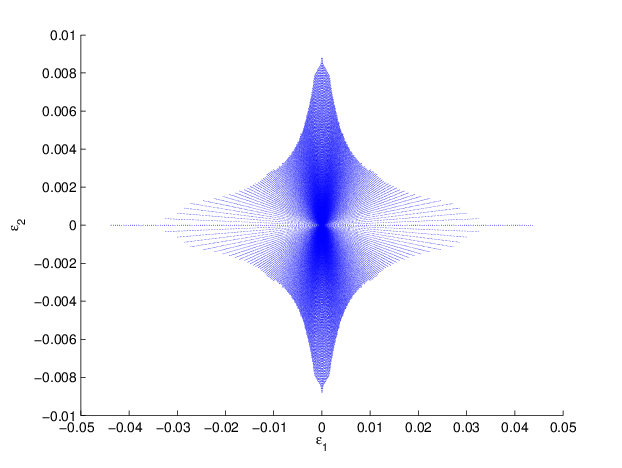
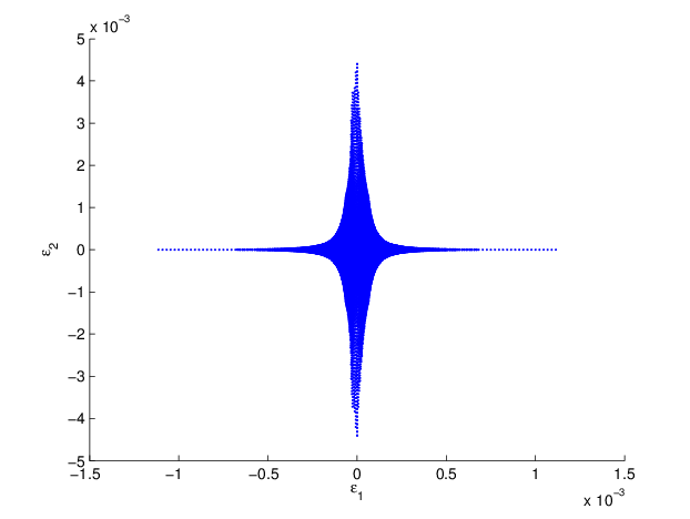
For a fixed rotation, we use the algorithm to explore rays in parameter space . In Figure 1 we plot the domains of analyticity for Models (4.1) and (4.2), that is, values of where the algorithm converged. The boundary of the domains of analyticity for each model appear to be smooth curves (at least locally). For Model (4.1) the domain appears to have reflection symmetries over both the and axes. Model (4.2) appears to only have reflection symmetry over the axis.
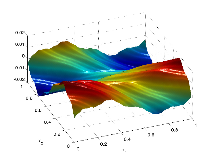
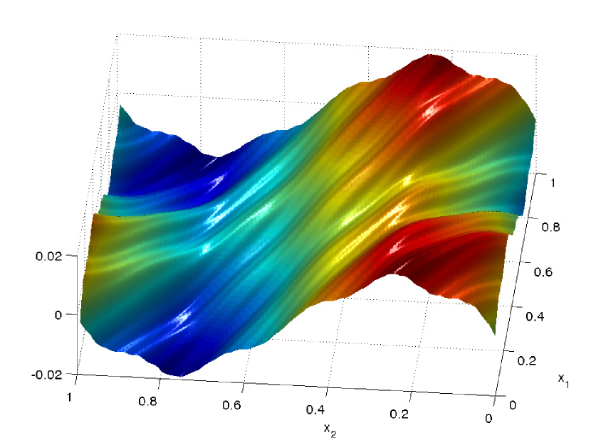
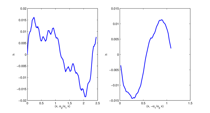
Figure 2 shows an invariant torus (from Model (4.1)) for parameter values near the breakdown of analyticity (2(a) and 2(b) are two different views of this torus). One can see that the torus oscillates rapidly in a single direction (this is the direction ). This “filamented” appearance indicates an anisotropic breakdown: the derivatives of blow up faster in the direction than they do in the direction . Figure 3 shows two curves that lie on the surface depicted in Figure 2. These curves are obtained by cutting the surface in Figure 2 along the directions and . Along, , we see fast oscillations (left graph) compared to the cut along (right graph). (A more quantitative description of the anisotropic breakdown is given in Figure 5, described below.)
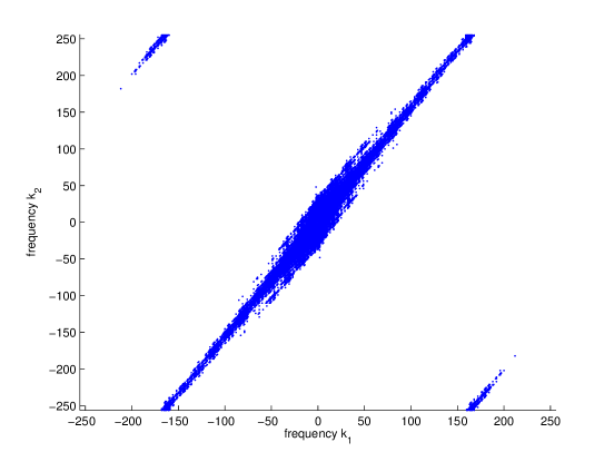
In Figure 4 we have depicted the indices for which the corresponding Fourier mode of the torus in Figure 2 is far from zero. We observe that the support of the Fourier transform is clustered along a line in Fourier space.
That means that the function can be aproximated by a function
which also lends credence to the belief that the result near breakdown is basically a one dimensional function.
Notice that, once we know that the final result is essentially a one dimensional function, it should be possible to perform linear changes of the variables so that this line is approximately parallel to one of the coordinate axis. Then, it would be more efficient to choose more Fourier modes along this direction. Of course, since our goal was to illustrate the appearence of this linear structure, we decided to use general algorithms that do not take advantage of its presence.
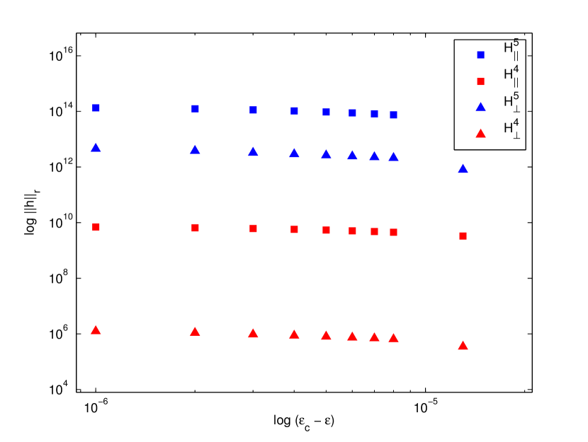
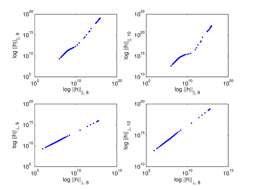
In Figure 5, we plot a log-log scale of the -norms and -norms (for ) versus , where is the critical value of along the line . We see that the -norms blow up much faster than the -norms, exhibiting the anisotropic breakdown.
In Figure 6(a), we plot against , and against for on log-log scales. As the parameters approach critical values, the log-log scale behavior is linear. (The -norm behaves like the -norm because of the anisotropic behavior.)
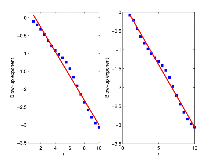
The blow-up behavior seen in Figure 5 fits a power-law form , with exponent depending on the order of the Sobolev norm. Computing the exponent for different values of , we find a nearly linear dependence on . In Figure 6(b) we plot the blow-up exponent for values as computed along two different lines in parameter space for Model (4.1). The blow-up exponent is for some constants . The fit-line in the left plot has and , while in right plot and . With higher-accuracy numerics, we expect to have similar plots for the -norms, too. These subdominant norms are measured with lower accuracy and more susceptible to noise in the numerics. We can see that they blow up like a power as approach the boundary of analyticity (Figure 5), but measuring the exponents as functions of the regularity will require more powerful numerics.
5. Conclusions
We have studied numerically the problem of breakdown of analyticity of hull functions in quasi-periodic media. This transition corresponds to the physical effect of transition between pinned down or sliding ground states.
Our computation has been carried out by efficient algorithms backed up by a-posteriori theorems that allow to compute confidently extremely close to the break up. We have uncovered certain regularities that, following the style of [Gre79], we call Assertions.
Assertion I The boundary of the domain of analyticity is a smooth curve (at least locally in the region explored).
Note that, following [AA80] this is analogous to what happens in phase transitions, where the phase transitions – which also correspond to a breakdown of analyticity – happen often in smooth surfaces (Gibbs rule) [Isr79]. The fact that the transitions happen locally in a smooth manifolds is one of the predictions of the renormalization group because they are the stable manifolds of a fixed point.
Of course, it can well happen that there are regions where the phase transition has cusps or other singularities, but we have not encountered them. It is, of course, quite conceivable that a more detailed exploration will uncover these singularities. As a cautionary tail, we mention that the paper [CdlL10b] uncovered singularities in the case of twist mappings that appeared only when a very large range of parameters was explored. The singularities are an indication that the renormalization group dynamics may have a more complicated behavior. Note that the apparent cusps found in Figure 1 near the coordinate axis are not real singularities. The potential has symmetries that the reflections along axis with the change in the origin.
Assertion II There are scaling behaviors near the blow up
We have seen that near the blow up we have
where (and perhaps too) is a universal number.
Actually, we have found a more precise version of scalings in each direction.
Assertion III The blow up of the norms is very anisotropic
If we define
we have near the breakdown
Moreover, when , we have:
Note that, as a particular case of the assertion, the tori remain somewhat regular up to the breakdown along lines.
Remark 5.1.
We think that it is also possible that there are scaling relations
with smaller exponents than those for the parallel norm. Unfortunately, verifying the above scaling relations is beyond reach at the moment. The fact that the asymptotic expansion is subdominant makes it harder to compute numerically (the calculations are contaminated by the larger effect) and also one can expect that this effect will manifest itself only much closer to breakdown.
Acknowledgements
Part of this work was done while the authors were affiliated with Univ. of Texas. We thank S. Hernandez and X. Su for many discussions about this problem and about numerical issues. We also thank the Center for Nonlinear Analysis (NSF Grants No. DMS- 0405343 and DMS-0635983), where part of this research was carried out.
References
- [AA80] Serge Aubry and Gilles André. Analyticity breaking and Anderson localization in incommensurate lattices. In Group theoretical methods in physics (Proc. Eighth Internat. Colloq., Kiryat Anavim, 1979), volume 3 of Ann. Israel Phys. Soc., pages 133–164. Hilger, Bristol, 1980.
- [ALD83] S. Aubry and P. Y. Le Daeron. The discrete Frenkel-Kontorova model and its extensions. I. Exact results for the ground-states. Phys. D, 8(3):381–422, 1983.
- [CC10] Renato Calleja and Alessandra Celletti. Breakdown of invariant attractors for the dissipative standard map. Chaos, 20(1):013121, 9, 2010.
- [CdlL09] Renato Calleja and Rafael de la Llave. Fast numerical computation of quasi-periodic equilibrium states in 1D statistical mechanics, including twist maps. Nonlinearity, 22(6):1311–1336, 2009.
- [CdlL10a] Renato Calleja and Rafael de la Llave. Computation of the breakdown of analyticity in statistical mechanics models: numerical results and a renormalization group explanation. J. Stat. Phys., 141(6):940–951, 2010.
- [CdlL10b] Renato Calleja and Rafael de la Llave. A numerically accessible criterion for the breakdown of quasi-periodic solutions and its rigorous justification. Nonlinearity, 23(9):2029–2058, 2010.
- [CF12] Renato Calleja and Jordi-Lluis Figueras. Collision of invariant bundles of quasi-periodic attractors in the dissipative standard map. Chaos, 23(02123), 2012.
- [CFL04] A. Celletti, C. Falcolini, and U. Locatelli. On the break-down threshold of invariant tori in four dimensional maps. Regul. Chaotic Dyn., 9(3):227–253, 2004.
- [dlL08] Rafael de la Llave. KAM theory for equilibrium states in 1-D statistical mechanics models. Ann. Henri Poincaré, 9(5):835–880, 2008.
- [FK39] J. Frenkel and T. Kontorova. On the theory of plastic deformation and twinning. Acad. Sci. URSS, J. Physics, 1:137–149, 1939.
- [FM12] Adam Fox and James D. Meiss. Critical asymmetric tori in the multiharmonic standard map, 2012.
- [GGP06] Jean-Marc Gambaudo, Pierre Guiraud, and Samuel Petite. Minimal configurations for the Frenkel-Kontorova model on a quasicrystal. Comm. Math. Phys., 265(1):165–188, 2006.
- [Gre79] J. M. Greene. A method for determining a stochastic transition. Jour. Math. Phys., 20:1183–1201, 1979.
- [GvE05] Guido Gentile and Titus S. van Erp. Breakdown of Lindstedt expansion for chaotic maps. J. Math. Phys., 46(10):102702, 20, 2005.
- [Her83] Michael-R. Herman. Sur les courbes invariantes par les difféomorphismes de l’anneau. Vol. 1, volume 103 of Astérisque. Société Mathématique de France, Paris, 1983. With an appendix by Albert Fathi, With an English summary.
- [HS99] A. Haro and C. Simó. A numerical study of the breakdown of invariant tori in 4D symplectic maps. In XIV CEDYA/IV Congress of Applied Mathematics (Spanish)(Vic, 1995), page 9 pp. (electronic). Univ. Barcelona, Barcelona, 199?
- [Isr79] Robert B. Israel. Convexity in the theory of lattice gases. Princeton University Press, Princeton, N.J., 1979. Princeton Series in Physics, With an introduction by Arthur S. Wightman.
- [KH95] Anatole Katok and Boris Hasselblatt. Introduction to the modern theory of dynamical systems, volume 54 of Encyclopedia of Mathematics and its Applications. Cambridge University Press, Cambridge, 1995. With a supplementary chapter by Katok and Leonardo Mendoza.
- [Koc04] Hans Koch. A renormalization group fixed point associated with the breakup of golden invariant tori. Discrete Contin. Dyn. Syst., 11(4):881–909, 2004.
- [LS03] Pierre-Louis Lions and Panagiotis E. Souganidis. Correctors for the homogenization of Hamilton-Jacobi equations in the stationary ergodic setting. Comm. Pure Appl. Math., 56(10):1501–1524, 2003.
- [Mac93] R. S. MacKay. Renormalisation in area-preserving maps, volume 6 of Advanced Series in Nonlinear Dynamics. World Scientific Publishing Co. Inc., River Edge, NJ, 1993.
- [Mat82] John N. Mather. Existence of quasiperiodic orbits for twist homeomorphisms of the annulus. Topology, 21(4):457–467, 1982.
- [Mat09] Daniel C. (ed.) Mattis. The many-body problem. An encyclopedia of exactly solved models in one dimension. 3rd printing with revisions and corrections. Hackensack, NJ: World Scientific. xxvi, 964 p., 2009.
- [MO00] B. D. Mestel and A. H. Osbaldestin. Periodic orbits of renormalisation for the correlations of strange nonchaotic attractors. Math. Phys. Electron. J., 6:Paper 5, 29 pp. (electronic), 2000.
- [Mos66] Jürgen Moser. A rapidly convergent iteration method and non-linear partial differential equations. I. Ann. Scuola Norm. Sup. Pisa (3), 20:265–315, 1966.
- [Mos86] Jürgen Moser. Monotone twist mappings and the calculus of variations. Ergodic Theory Dynam. Systems, 6(3):401–413, 1986.
- [Per79] I. C. Percival. A variational principle for invariant tori of fixed frequency. J. Phys. A, 12(3):L57–L60, 1979.
- [Rue69] David Ruelle. Statistical mechanics: Rigorous results. W. A. Benjamin, Inc., New York-Amsterdam, 1969.
- [Rüs75] Helmut Rüssmann. On optimal estimates for the solutions of linear partial differential equations of first order with constant coefficients on the torus. In Dynamical systems, theory and applications (Rencontres, Battelle Res. Inst., Seattle, Wash., 1974), pages 598–624.Lecture Notes in Phys., Vol. 38. Springer, Berlin, 1975.
- [Rüs76] Helmut Rüssmann. Note on sums containing small divisors. Comm. Pure Appl. Math., 29(6):755–758, 1976.
- [SdlL12a] Xifeng Su and Rafael de la Llave. KAM theory for quasi-periodic equlibria 1-D quasiperiodic media. SIAM Jour. Math. Anal., 14:3901–3927, 2012. MP_ARC #11-56.
- [SdlL12b] Xifeng Su and Rafael de la Llave. KAM theory for quasi-periodic equlibria in one dimensional quasiperiodic media: II extended range interactions. Jour. Phys. A, 45:45203, 2012.
- [Tom96] Stathis Tompaidis. Numerical study of invariant sets of a quasiperiodic perturbation of a symplectic map. Experiment. Math., 5(3):211–230, 1996.
- [vE99] T. S. van Erp. Frenkel Kontorova model on quasiperiodic substrate potentials. 1999. Thesis.
- [vEF02] T. S. van Erp and A. Fasolino. Aubry transition studied by direct evaluation of the modulation functions of infinite incommensurate systems. Europhys. Lett., 59(3):330–336, 2002.
