The Atacama Cosmology Telescope: likelihood for small-scale CMB data
Abstract
The Atacama Cosmology Telescope has measured the angular power spectra of microwave fluctuations to arcminute scales at frequencies of 148 and 218 GHz, from three seasons of data. At small scales the fluctuations in the primordial Cosmic Microwave Background (CMB) become increasingly obscured by extragalactic foregounds and secondary CMB signals. We present results from a nine-parameter model describing these secondary effects, including the thermal and kinematic Sunyaev-Zel’dovich (tSZ and kSZ) power; the clustered and Poisson-like power from Cosmic Infrared Background (CIB) sources, and their frequency scaling; the tSZ-CIB correlation coefficient; the extragalactic radio source power; and thermal dust emission from Galactic cirrus in two different regions of the sky. In order to extract cosmological parameters, we describe a likelihood function for the ACT data, fitting this model to the multi-frequency spectra in the multipole range . We extend the likelihood to include spectra from the South Pole Telescope at frequencies of 95, 150, and 220 GHz. Accounting for different radio source levels and Galactic cirrus emission, the same model provides an excellent fit to both datasets simultaneously, with /dof= for ACT, and for SPT. We then use the multi-frequency likelihood to estimate the CMB power spectrum from ACT in bandpowers, marginalizing over the secondary parameters. This provides a simplified ‘CMB-only’ likelihood in the range for use in cosmological parameter estimation.
Subject headings:
cosmology: cosmic microwave background, cosmology: observations1. Introduction
Measurements of the Cosmic Microwave Background (CMB) have played a central role in constraining cosmological models. Anisotropies measured over the whole sky by WMAP have provided evidence for a flat universe described by just six cosmological parameters. The measurement of the Sachs-Wolfe plateau in the power spectrum, and three acoustic peaks, have led to constraints on CDM parameters to percent-level accuracy (Komatsu et al., 2011; Larson et al., 2011). The Silk damping tail of the power spectrum provides a wealth of additional information about the physics of the early universe, encoded in its shape, and in the positions and heights of the higher-order acoustic peaks (Silk, 1968). Extracting information from these angular scales is complicated by the presence of additional power from extragalactic point sources, emission from the Galaxy, and secondary anisotropies due to the thermal and kinematic Sunyaev-Zel’dovich effects (Sunyaev & Zel’dovich, 1970).
The Atacama Cosmology Telescope (ACT) mapped the mm-wave sky with arcminute resolution from 2007 to 2010 in two distinct areas. About 600 square degrees were used to compute the angular power spectrum. Power spectra and cosmological results using the 1-year data, from the 2008 observing season, were presented in Fowler et al. (2010); Das et al. (2011); and Dunkley et al. (2011). During roughly the same period, the South Pole Telescope also mapped the microwave sky, and presented cosmological results in Lueker et al. (2010); Shirokoff et al. (2011); Keisler et al. (2011); Reichardt et al. (2012); and Story et al. (2012).
In this paper we describe a method to fit multi-frequency power spectra from the ACT data simultaneously for CMB, foreground, and SZ parameters, following a similar approach to analyses in Dunkley et al. (2011) and Reichardt et al. (2012). We describe the likelihood constructed for the 3-year ACT dataset, using data from the 2008-2010 observing seasons, and show how it can be used in combination with data from SPT in a self-consistent way. Using this likelihood from ACT, we then construct a simpler CMB-only likelihood, estimating CMB bandpowers marginalized over the SZ and foreground parameters.
This is one of a set of papers on the 3-year ACT data; Das et al. (2013) present the angular power spectra, and Sievers et al. (2013) use the likelihoods presented here to estimate cosmological parameters. We begin in §2 by describing the model for the mm-wave emission. In §3 the full likelihood of the ACT data is described, including the combination with data from SPT and WMAP 7-year data. In §4 we show the small-scale model fit to the multi-frequency data. In §5 we describe the compressed CMB-only likelihood, concluding in §6.
2. Model for the mm-wave sky
| Dataset | Frequencyaafootnotemark: | Reference | Area | bbfootnotemark: | ccfootnotemark: | ||||
| GHz | sq degrees | mJy | GHz | GHz | GHz | ||||
| ACT | 148 | Das et al. (2013) | 590ddfootnotemark: | 500 | 10000 | 15 | 146.9 | 147.6 | 149.7 |
| 218 | 1500 | 10000 | 220.2 | 217.6 | 219.6 | ||||
| SPT-low | 150 | Keisler et al. (2011) | 790 | 650 | 2000 | 50 | 152.9 | 150.2 | 153.8 |
| SPT-high | 95 | Reichardt et al. (2012) | 800 | 2000 | 9400 | 97.6 | 95.3 | 97.9 | |
| 150 | 2000 | 9400 | 6.4 | 152.9 | 150.2 | 153.8 | |||
| 220 | 2000 | 9400 | 218.1 | 214.1 | 219.6 | ||||
| 11footnotetext: All cross-spectra between channels are used in the likelihood. 22footnotetext: Flux cut imposed on map by its point source mask. 33footnotetext: Effective band-centers from ACT are from Swetz et al. (2011), given for tSZ, radio sources, and CIB sources. 44footnotetext: This area includes the ACT-E region at dec (300 deg2), and the ACT-S region at dec (290 deg2). |
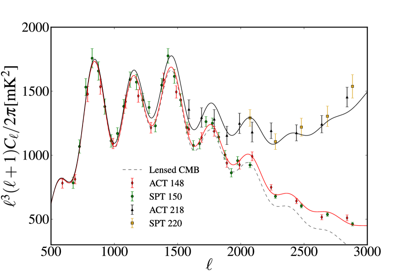
Sky maps of mm-wave fluctuations at arcminute resolution include components emitting at low redshift, in addition to the primordial CMB signal and secondary CMB effects (e.g., Sievers et al., 2009; Fowler et al., 2010; Dunkley et al., 2011; Keisler et al., 2011). The power spectra from the complete ACT dataset, reported in Das et al. (2013), are shown in Figure 1, focusing on angular scales of interest for the primordial CMB signal. At scales smaller than a few arcminutes () the secondary signal, which we define as the sum of foregrounds and SZ effects, becomes significant compared to the CMB. We want to extract the primary CMB signal, but, since there are more foreground components than frequency channels, information about both the frequency and scale dependence of the foregrounds is required to separate the signals. In this section we describe a model to fit the power spectrum of these fluctuations over the frequency range GHz probed by ACT, SPT, and other CMB experiments including the Planck satellite (Planck Collaboration I et al., 2011). We follow a similar approach to Sievers et al. (2009); Dunkley et al. (2011); Reichardt et al. (2012).
For frequency and direction we model the signal in the maps as
| (1) |
where are the lensed CMB fluctuations, which are independent of frequency in thermodynamic units. The secondary signal, , is dominated by the sum of tSZ and kSZ components, emission from dusty infrared galaxies and radio galaxies, and dust emission from Galactic cirrus, all of which are functions of frequency.
The cross-correlation power spectra between frequency and are calculated as
| (2) |
where is the Fourier transform of in the flat-sky approximation. The theoretical cross-spectrum is modeled as
| (3) |
where is the lensed primary CMB power spectrum. In this analysis we model the secondary spectra as
| (4) | |||||
with contributions from the tSZ and kSZ effects; dusty galaxies that form part of the Cosmic Infrared Background, both Poisson-like (CIB-P) and clustered (CIB-C); the cross-correlation between the tSZ effect and the CIB (tSZ-CIB); radio galaxies (rad); and dust emission from Galactic cirrus (Gal). We assume that all other cross-spectra can be neglected. Measurements by WMAP and other CMB experiments show that other Galactic emission, including synchrotron and free-free emission, is negligible in the GHz frequency range at these small scales and locations (e.g., Gold et al., 2011). The cross-correlation of radio sources and both tSZ and CIB sources is also expected to be small (e.g., Sehgal et al., 2010, who find a correlation of only a few per cent in simulations). Since the kSZ signal consists of positive and negative fluctuations, depending on the line-of-sight motion of the electrons that source the signal, the two-point correlation function with other signals should average to zero.
The majority of these secondary spectra will be common to all regions of the sky and to different experiments. The power in the residual radio point sources is expected, however, to vary among data sets due to the removal of bright sources. For example, for a Poisson distribution of sources with differential number counts scaling as , the Poisson power will be
| (5) |
i.e., , where is the flux of the brightest sources in the map at a given frequency. Deeper surveys, with lower noise per pixel, are able to detect and mask out dimmer sources, so will be lower, leading to a lower residual power. Radio sources have a shallower slope than CIB galaxies, so imposing a flux cut of, e.g., mJy removes a significant amount of radio power, but little CIB power.
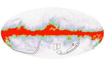
The Galactic foreground power is also expected to vary between regions on the sky. The two regions mapped by ACT (Equatorial, ACT-E, and South, ACT-S) are shown in Figure 2 and summarized in Table 1, together with data from SPT. The temperature scale of the Galactic cirrus map from Finkbeiner et al. (1999) is shown for comparison. A higher level of emission is expected in some regions of the ACT-E region.
In the rest of this section we describe how each of the components in Eq. 4 are modeled. To allow for comparisons between experiments, we normalize the power spectra at a pivot frequency of GHz and scale . This differs slightly from the convention used in previous analyses of the ACT data (Fowler et al., 2010; Dunkley et al., 2011). In each case we describe the parameterization used in the fiducial model; in a later section we consider possible extensions or modifications.
2.1. Thermal Sunyaev-Zel’dovich
Our model for the power from thermal SZ fluctuations is given by
| (6) |
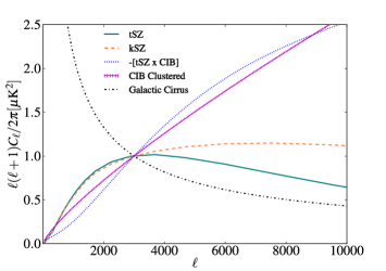
where is a template power spectrum corresponding to the predicted tSZ emission at for a model with amplitude of matter fluctuations , normalized to K2 at , and is a free parameter describing its amplitude. An example is shown in Figure 3. The factor , for , scales the expected tSZ emission to thermodynamic units at , the effective band-center for the tSZ, given in Table 1. We ignore relativistic corrections (e.g., Itoh et al., 1998), since the low-mass clusters that dominate the spectra are well approximated by the non-relativistic formula. This normalization differs from that used in Dunkley et al. (2011). The present choice has the advantage of reducing the dependence on the choice of template, since the main difference between various templates is their amplitude. This means one expects to find the same constraint on regardless of template, and a constraint on the SZ power can be converted back into a model-dependent constraint on .
The template we adopt is derived from recent hydrodynamic simulations described in Battaglia et al. (2012a). The simulations include the effects of radiative cooling, star formation, and feedback from AGN and supernovae. The predictions are consistent with SZ measurements from both SPT and ACT (e.g., Lueker et al., 2010), and the shape is shown in Figure 3. For the model with , the predicted spectrum reported in Battaglia et al. (2012a) has amplitude , with standard deviation estimated from ten simulations.
Numerous other authors have also predicted the tSZ spectrum from independent simulations and analytical models (e.g., Komatsu & Seljak, 2002; Shaw et al., 2009; Sehgal et al., 2010; Trac et al., 2011; Shaw et al., 2010; Battaglia et al., 2012a; Efstathiou & Migliaccio, 2012), and the expected amplitude for fixed cosmological model varies depending on the astrophysical modeling of the clusters. However, the template shape is broadly consistent among models, and the data are not yet sensitive to shape difference, so we do not include a shape uncertainty. We do not mask clusters, and expect the total SZ power to be the same for ACT and SPT.
2.2. Kinematic Sunyaev-Zel’dovich
The kSZ power is expected to have contributions arising from fluctuations in the electron density (Ostriker & Vishniac, 1986), and in the ionization fraction (e.g., Gruzinov & Hu, 1998; McQuinn et al., 2005; Iliev et al., 2007), as well as from the motion of galaxy clusters at later times. We model the power as
| (7) |
where is a template spectrum for the predicted blackbody kSZ emission for a model with , normalized to at . The parameter describes its normalization. We use a template that assumes a model with instantaneous reionization, described in Battaglia et al. (2010). This is derived from the same hydrodynamic simulations as the tSZ spectra in Sec 2.1, and is shown in Figure 3. The predicted amplitude from the simulations is for homogeneous reionization at in a cosmology. This is a quarter of the expected tSZ power. The corresponding kSZ template for the ‘nonthermal20’ model in Trac, Bode, & Ostriker (2011) has a similar amplitude and shape, as does the Shaw, Rudd, & Nagai (2012) ‘CSF’ model, and the Bode et al. (2012) model. The power is expected to scale as roughly (Trac et al., 2011; Shaw et al., 2012)).
Reionization of the universe is not expected to be instantaneous, as was assumed by Battaglia et al. (2010). The shape and amplitude of the kSZ power from patchy reionization is far less certain, with simulations predicting a signal at least as large as the homogeneous signal (e.g., Zahn et al., 2012; Mesinger et al., 2012; Battaglia et al., 2012b). This gives a total expected signal of to for simple reionization models at , comparable to the tSZ at 150 GHz. The dominant effect of patchy reionization on the power spectrum at scales probed by ACT is to alter the amplitude, depending on both the midpoint and duration of reionization (e.g., Battaglia et al., 2012b). We test a modified shape in §4.3, but do not include additional shape uncertainty in the template in the basic model.
2.3. Cosmic infrared background
Thermal dust emission from high redshift star-forming galaxies, part of the Cosmic Infrared Background (CIB), is emitted in the rest-frame far infrared and redshifted into the mm-wave range (e.g., Puget et al., 1996; Hauser et al., 1998). Clustering of these galaxies has been detected statistically in mm-wave maps at CMB frequency (Hall et al., 2010; Dunkley et al., 2011; Shirokoff et al., 2011; Planck Collaboration XVIII et al., 2011; Hajian et al., 2012; Reichardt et al., 2012), as well as in the sub-mm (e.g., Lagache et al., 2007; Viero et al., 2009). Following the analyses in Dunkley et al. (2011); Reichardt et al. (2012); Addison et al. (2012b), the power from these galaxies is modeled as the sum of a Poisson and clustered component, given by
| (8) |
for the Poisson part, and
| (9) |
for the clustered part. Here, is a power law index, and the frequency scaling of each component is given by a modified blackbody,
| (10) |
with emissivity indices and for the Poisson and clustered dust terms respectively. The function is the Planck function at frequency for effective dust temperature , and the function converts from flux to thermodynamic units. The parameters and normalize the two components at and , and different frequencies channels are assumed to be perfectly correlated.
The frequency dependence we adopt is an approximation to a sum of modified blackbodies at different redshifts, so this emissivity and temperature are only effective properties of the dust. Following Addison et al. (2012b) we fix the dust effective temperature to K. We also assume in the basic model.
The power-law angular scaling of the clustered term, with increasing power at small scales, is shown in Figure 3, and approximates the shape of the non-linear power spectrum, which includes contributions from pairs of galaxies in the same dark matter halo, and between galaxies in different halos. Addison et al. (2012b) find that a power law in provides a good fit to small-scale power spectra from Planck and the Balloon-borne Large-Aperture Submillimeter Telescope (BLAST), and from cross-correlating ACT and BLAST maps. This is consistent with observations of the correlation function from high-redshift Lyman break galaxies, as well as local galaxies (e.g., Giavalisco et al., 1998; Connolly et al., 2002). We fix the power-law index to in the fiducial case (), in close agreement with the estimate of in Addison et al. (2012b). Both are in agreement with galaxy correlation functions.
We do not expect the CIB power to vary significantly between the ACT and SPT maps, despite the different flux cuts applied to remove sources. Using the model in Addison et al. (2012a), the predicted effect of source masking on the CIB power is only at the per cent level.
2.4. tSZ-CIB cross-correlation
Some spatial correlation is expected between clusters that contribute to the tSZ, and CIB galaxies, since both trace the matter density field. The higher redshift and lower mass groups that make an important contribution to the tSZ signal (Komatsu & Seljak, 2002; Trac et al., 2011; Battaglia et al., 2012b) are also likely to host dusty galaxies. Addison et al. (2012c) model this correlation, and predict the scale and frequency dependence of its angular power spectrum. For mm-wave spectra at , a correlation of to % in power is predicted, with uncertainty dominated by uncertainties in the halo mass and redshift distribution of the CIB. A significant fraction of the CIB power on small scales is due to pairs of galaxies occupying group and cluster-mass halos (the ‘one-halo’ term of the halo model). These same halos are responsible for the tSZ power. A tSZ-CIB correlation in units of power of tens of per cent is therefore possible on small angular scales even if the overall fraction of CIB emission associated with massive halos is small.
The tSZ-CIB power is negative at 150 GHz, and can partially cancel power from the kSZ effect as it does not vary significantly with frequency over the range probed by ACT and SPT. As a result, neglecting this component can lead to artificially tight constraints on the kSZ power (Zahn et al., 2012; Mesinger et al., 2012). Following Addison et al. (2012b) we model the spectrum as
| (11) |
where is the predicted correlation spectrum shape, normalized to at and shown in Figure 3. The free parameter is the correlation coefficient. The Poisson CIB parameter is not included in Eq. 11, unlike in Shirokoff et al. (2011); Zahn et al. (2012), as the sources that dominate the CIB Poisson power in the mm-wave bands are unlikely to have significant redshift-overlap with the tSZ clusters (Addison et al., 2012c). Assuming the same modified blackbody scaling for the CIB as in §2.3, and tSZ frequency scaling , the frequency scaling of the cross-spectra in thermodynamic units is then
| (12) |
for pivot scale .
Since the correlation coefficient is poorly constrained by ACT, we impose a uniform prior of in the basic model; the effect of widening the range to e.g., , corresponding to the maximum allowed correlation in the models explored by Addison et al. (2012c), is discussed in Sievers et al. (2013). Due to the correlation between and the kSZ power, broadening the limit on increases the upper limit on the kSZ power, but does not affect cosmological results.
2.5. Radio point sources
The radio sources at ACT frequencies are not expected to be significantly clustered (see e.g., Sharp et al., 2010; Hall et al., 2010), and to good approximation their power should be perfectly correlated between neighbouring frequencies, consistent with simulations in Sehgal et al. (2010) and valid for sources with the same spectral indices. As in Dunkley et al. (2011) and Reichardt et al. (2012), we model the residual power after masking bright sources as Poisson scale-free power, with
| (13) |
in thermodyamic units, where converts from flux units as for the CIB sources. The amplitude is normalized at and . Measurements of bright sources from ACT and SPT give an estimate for the spectral index in flux units of typically (Vieira et al., 2010; Marriage et al., 2011). Assuming it holds at fainter fluxes, we fix in the fiducial model.
Bright source counts can also be used to predict by extrapolating to fainter fluxes using a model for the number of sources as a function of flux. This was done in Marriage et al. (2011) for ACT, and for SPT in Keisler et al. (2011); Reichardt et al. (2012). Using point sources measured from the full ACT dataset, Gralla et al. (2013) now predict a residual power after masking sources brighter than 15 mJy in both ACT regions (the level used to construct the mask for our maps in this analysis), where the catalog is estimated to be complete. We impose this as a Gaussian prior on the power at 150 GHz. For comparison, the estimated power in the SPT power spectra after masking to a flux level of 6 mJy for SPT-high is (Reichardt et al., 2012), which we also impose as a Gaussian prior.
2.6. Residual Galactic cirrus
The Galactic emission is spatially varying, and Das et al. (2013) show that dust emission can contribute significantly to the power spectra, particularly in our Equatorial region. As reported in Das et al. (2013), we apply a mask to regions of high dust emission before computing the power spectrum, using measurements at 100 from IRIS (Miville-Deschênes & Lagache, 2005).
We then marginalize over a residual Galactic cirrus component using a power-law template
| (14) |
with amplitude , frequency index , and angular scaling . This angular scaling is estimated from the 100 IRIS dust maps (Miville-Deschênes & Lagache, 2005). The frequency scaling is estimated by correlating the IRIS dust maps with ACT (Das et al., 2013), and is consistent with early results from Planck (Planck Collaboration XIX et al., 2011). Using the correlation coefficients estimated in Das et al. (2013), we impose priors of , and in the ACT-E and ACT-S spectra respectively.
For the SPT data, a small Galactic cirrus residual is also expected. In our basic model we follow the treatment in Reichardt et al. (2012), fixing the Galactic cirrus power to , , and in thermodynamic units at 95, 150, and 220 GHz, with scale dependence . However, this model has a steeper angular power law than in our ACT model, and a shallower frequency scaling ( between 150–220 GHz). For consistency we therefore test the effect of adopting the ACT model instead, using and , and a prior of . We find no effect on parameters and no change in the goodness of fit.
3. Full likelihood from small-scale data
In this section we describe the multi-frequency likelihood used to model the ACT data, and show how we extend it to include other small-scale datasets, in particular data from SPT.
3.1. Likelihood from the ACT data
The data from Das et al. (2013) describe the two ACT regions separately (ACT-E and ACT-S); and consist of multi-season and multi-frequency spectra, with an associated covariance matrix111In this paper we use the original version ‘v1’ of the spectra, unless stated. Since original release, the binning and the beams have been slightly refined, generating ‘v2’ of the spectra. This is described in Das et al. (2013), and the ‘v2’ spectra are released publicly; cosmological effects are negligible as described in Sievers et al. (2013).. They are derived from ACT maps obtained using the method described in Dünner et al. (2012). The likelihood is Gaussian-distributed to good approximation. To construct the likelihood for each region, given some model spectra , we compute bandpower theoretical spectra using , where is the bandpower window function in band for cross-spectrum , described in Das et al. (2013).
The likelihood, , of the data for each ACT region separately is given by
| (15) |
where is the bandpower covariance matrix. Each of the model and data vectors and contain three sets of spectra,
for ACT-E and ACT-S separately, and each spectra set itself contains spectra for each cross-season. There are two seasons used for ACT-E (3 cross-season spectra), and three for ACT-S (6 cross-season spectra). The total likelihood is given by
3.1.1 Calibration and beam uncertainty
The data power spectra are calibrated, but have uncertainties. We therefore include a calibration parameter , for each map , that scales the estimated data power spectra as
and the elements of the bandpower covariance matrix as
To account for both ACT regions, we include four calibration parameters: , for ACT-E at 148 GHz and 218 GHz, and , for ACT-S.
Das et al. (2013) calibrate the 148 GHz maps using WMAP, following the method in Hajian et al. (2011), at an effective , resulting in a 2% map calibration error in CMB temperature units. We impose this as a Gaussian prior, with . The 218 GHz maps are calibrated relative to 148 GHz, at an effective . The 218 GHz calibration is constrained by the cross-spectrum, so no prior is imposed on and . Within each frequency, the individual seasons are calibrated to each other; the inter-season calibration error is absorbed into the single overall calibration uncertainty.
Uncertainties in the measured beam window functions for ACT at 148 GHz are between 0.7 and 0.4%, and at 218GHz between 1.5 and 0.7%. We incorporate uncertainties in the measured beams by including them directly in the covariance matrix for the spectra, described in Das et al. (2013). This technique assumes a fiducial model for the power spectra but is insensitive to its exact form.
3.1.2 Secondary model parameters
Our model described in Section 2 has nine free secondary parameters for ACT in the basic case: and describing the SZ emission, , and describing the CIB power, describing the radio power, describing the tSZ-CIB cross-correlation, and and describing the Galactic cirrus emission. The latter four have strong priors imposed, as described in §2: , , , and . In addition to the nine model parameters, there are four calibration parameters for ACT. In §4.3 we investigate how additional, or fewer, parameters affect the fit of the model to the data. To compute the model requires an effective frequency for each component; we use the band-centers for SZ, radio, and dusty sources given in Table 1 (Swetz et al., 2011).
3.2. Combining with SPT data
The South Pole Telescope observed the sky from 2007–10. Spectra are reported in Keisler et al. (2011) for angular scales at 150 GHz, and in Reichardt et al. (2012) for angular scales at 95, 150 and 220 GHz. These observations are summarized in Table 1. One of the goals of our work here is to test for consistency between the two experiments, by using a common framework to describe the SZ and foreground components. As this article was being prepared, refined spectra from SPT at 150 GHz were reported in Story et al. (2012); we do not include these latest data in our comparison.
Before fitting the SPT data with the ACT secondary model, we confirm that we recover the parameters and obtained for the model used in Reichardt et al. (2012) using the SPT data. To combine the data over the full angular range, we follow the method in Reichardt et al. (2012), using the Keisler et al. (2011) data at (SPT-low) and the Reichardt et al. (2012) data at smaller scales (SPT-high). More radio source power has been removed from the SPT-high spectra due to masking at a deeper flux level, so the expected residual radio power in SPT-low is K2, compared to for SPT-high. We account for this by first subtracting a radio Poisson power of from the SPT-low data, following the approach in Reichardt et al. (2012). A Gaussian prior is then imposed on the overall residual radio level in SPT of .
We then extend the ACT secondary model to fit the SPT power spectra. Six of the ACT model parameters are expected to be common for the SPT data (the SZ and CIB parameters: , , , , and ). In addition, to fit the SPT data we require a separate radio source parameter, , and three calibration parameters, , , , to calibrate the 95, 150, and 220 GHz maps respectively. We impose a uniform prior on these calibration parameters, as the SPT covariance matrices include the calibration uncertainty.
The likelihood for ACT and SPT together is given by
| (16) |
The SPT likelihood is constructed as in Eq. 15, with model and data vectors
| (17) |
for SPT-high at , and for SPT-low at . To compute the model, we use the band-centers for SZ, radio and dusty sources given in Table 1, from Reichardt et al. (2012).
There is some degree of covariance between the ACT and SPT spectra, due to the 54 deg2 overlapping region of sky. Covariance between the two spectra due to cosmic variance, scaling as , is estimated at a level of 8% (using ); the addition of noise lowers this level, so we neglect the correlation in our combined analysis.
3.3. Multi-frequency likelihood prescription
To return the ACT (or ACT+SPT) multi-frequency likelihood for a given model we follow this approach:
-
•
Select primary cosmological parameters, and compute a theoretical lensed CMB power spectrum using the CAMB numerical Boltzmann code (Lewis et al., 2000).
-
•
Select values for common secondary parameters: , , , , , }.
-
•
Select values for ACT-specific secondary and calibration parameters: , , , , , , }, and/or SPT-specific secondary and calibration parameters: , , , }.
-
•
Compute the total theoretical secondary power spectra for all the required cross-spectra with Eq. 4, using the effective frequencies for each experiment.
-
•
Compute the total model power at each frequency, .
-
•
Compute the bandpower theoretical power spectra for each dataset for both South and Equatorial regions for ACT (and for SPT), and compute the likelihood using Eq. 3.1.
3.3.1 Combining with WMAP
In Sievers et al. (2013) we use the ACT and SPT likelihood in combination with data from WMAP seven-year data to estimate cosmological parameters. The WMAP data measure angular scales, and so have minimal contamination from SZ and point sources. The public 7-year likelihood estimates the temperature spectrum from V and W bands (61 and 94 GHz, Larson et al., 2011). At these frequencies and angular scales, the infrared point source contribution is expected to be negligible, consistent with ACT and SPT measurements. The radio point source level is estimated and subtracted internally to the WMAP analysis using the multi-frequency data (e.g., Nolta et al., 2009). Finally, in light of observations by both ACT and SPT, we also neglect the SZ power in the WMAP data, as it is expected to be small: K2 at 61 GHz from the Battaglia et al. (2012a) model, assuming .
4. Tests of the multi-frequency likelihood
In this section we test the goodness of fit of the model to the ACT power spectra, assuming the CDM cosmological model. We estimate the probability distributions of the secondary parameters using the MCMC method described in Dunkley et al. (2011), fixing the CDM parameters at best-fitting values222Physical baryon density , cold dark matter density , ratio of the acoustic horizon to the angular diameter distance at decoupling , scalar amplitude , spectral index , and optical depth .. We then investigate a set of possible extensions or modifications to the secondary model. We include the SPT power spectra and examine the consistency of the foreground model between the two datasets. We use the ACT ‘v1’ spectra for this analysis; as described earlier, a refined estimate of the beams became available after the analysis was complete. We have checked that effects on parameters are negligible (), so do not update the parameter constraints or plots in this section.
4.1. ACT data
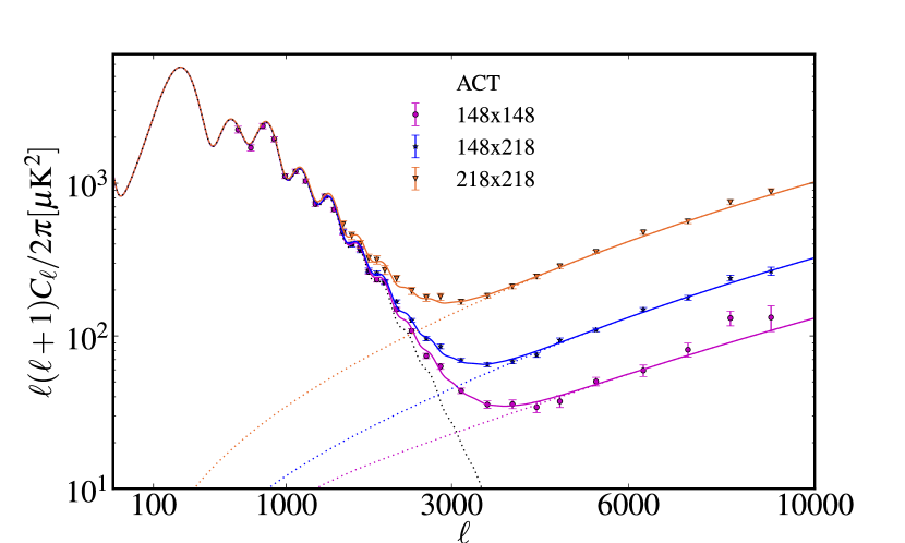
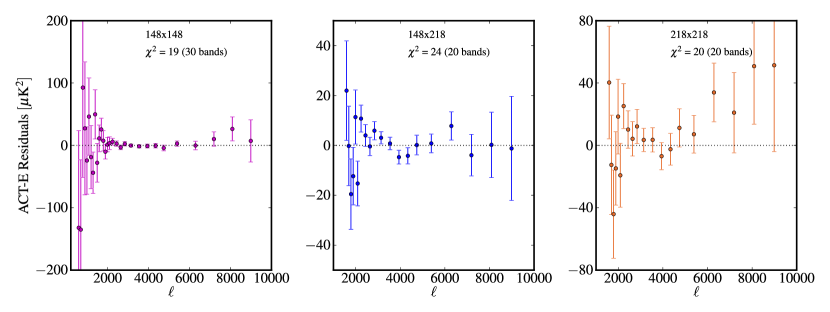
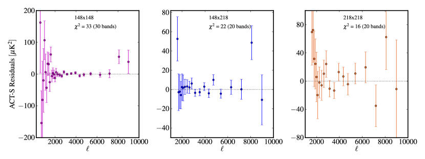
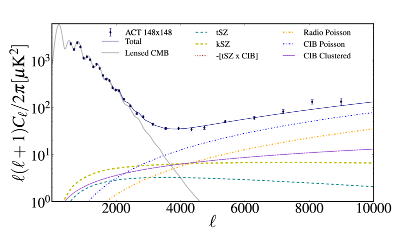
We find that the model provides a good fit to the ACT data over the full range of angular scales and frequencies. Figure 4 shows the total spectra (coadded over ACT-E and ACT-S, with the best-fitting Galactic cirrus component removed) decomposed into primary and secondary contributions. The SZ and foregrounds dominate at at 218 GHz, and at at 148 GHz. The goodness of fit is for dof (reduced , with PTE, for 710 data points and 13 parameters). This indicates a good overall fit, but localised deviations can be hard to identify using the over the full angular range. Figure 4 therefore shows the residual power after subtracting the best-fitting model; we do not observe any significant features, indicating that the model fits both the angular and frequency dependence of the data in both regions. There is a positive excess in the ACT-E residuals at the smallest scales at 218 GHz, but this is consistent with correlated beam error, accounted for in the covariance matrix.
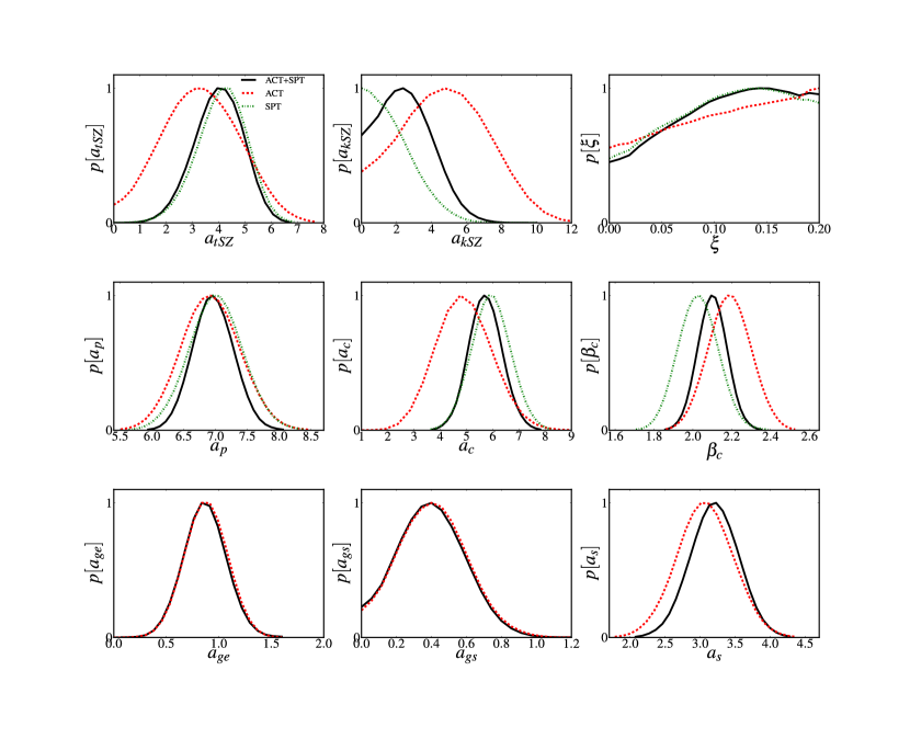
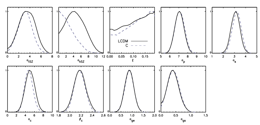
The marginalized distributions for the secondary parameters fitting the data are shown in Figure 5 and summarized in Table 2. The Poisson-like and clustered CIB power, and , are detected at high significance, with index consistent with Addison et al. (2012b) who find . The tSZ and kSZ power are individually seen at low significance, with an anti-correlation between and . The kSZ power peaks at a non-zero value, but the distribution is broad and consistent with zero. The total SZ power is detected at high significance. The tSZ-CIB correlation coefficient is unconstrained in the prior range , and is also unconstrained by ACT if allowed to vary over a broader range (e.g., ). The parameters for the power from radio sources and from Galactic cirrus are driven by their prior distributions. Sievers et al. (2013) present a physical interpretation of these parameters; the constraints are consistent with those found in the 1-year ACT analysis in Dunkley et al. (2011), with reduced errors.
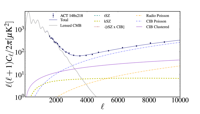
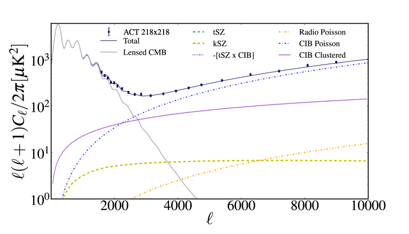
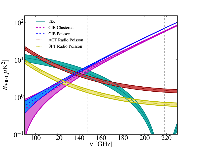
In Figure 6 we show the individual components that contribute to the 148 GHz and 218 GHz power spectra after removal of the best-fitting Galactic cirrus power. At 148 GHz there are contributions from all the components. At 218 GHz the secondary spectrum is dominated by dusty point sources, both clustered and Poisson. This is illustrated further in Figure 7, which shows the frequency dependence of the dominant components in our model at . The derived constraints on the CIB and radio source components, and the Galactic cirrus emission, at the ACT effective frequencies are also given in Table 3 to allow comparison with other models.
| Parameter | Priorbbfootnotemark: | ACTccfootnotemark: | SPT | ACT+SPT | |
| SZ | |||||
| ddfootnotemark: | |||||
| CIB | |||||
| tSZ-CIB | |||||
| Radio | — | ||||
| — | |||||
| Galactic cirruseefootnotemark: | — | ||||
| — | |||||
| Calibration | — | ||||
| — | — | ||||
| — | |||||
| — | — | ||||
| — | — | ||||
| — | — | ||||
| — | — | ||||
| best fit /dof | |||||
| PTE |
| ACT | SPT | ||||
|---|---|---|---|---|---|
| 148 GHz | 218 GHz | 95 GHz | 150 GHz | 220GHz | |
| CIB-P | 78 | ||||
| CIB-C | |||||
| Radio | |||||
| Gal-Eaafootnotemark: | |||||
| Gal-S | |||||
4.2. Combination with SPT
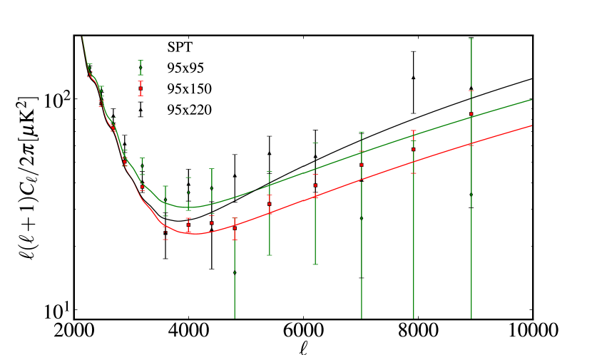
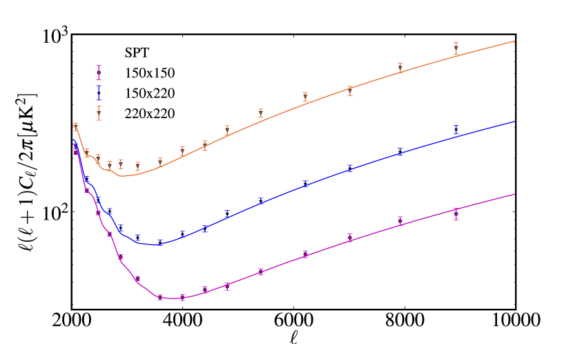
The same model also provides a good fit to the SPT spectra. The SPT data extend the frequency range to 95 GHz, adding three additional cross-spectra to the likelihood. We show the parameters estimated from SPT alone in Figure 5 and in Table 2; they are consistent with those from ACT, with shifts in and . The radio Poisson level is lower due to the greater number of radio sources masked in the SPT maps. The model is shown with the SPT spectra in Figure 8; the goodness of fit is for dof (reduced , PTE=0.77).
Given the consistency of the two datasets, we combine them to generate a joint likelihood; Figure 5 includes the secondary parameters derived from a joint fit. In this case there are ten foreground parameters, and seven calibration parameters. The tenth foreground parameter (not plotted) is for the Poisson radio sources in SPT. The goodness of fit of the joint model is , which can be compared to for the independent fit to each data set. This supports their consistency.
We report the derived constraints on the CIB and radio source components at the ACT and SPT effective frequencies for each band in Table 3. A difference of approximately 15% is expected between the CIB power at 148 GHz for ACT and 150 GHz for SPT, due to different effective bandpass frequencies and the strong CIB frequency dependence across the mm-wave bands.
4.3. Tests of the likelihood
| Model | Number of | ACTbbfootnotemark: |
|---|---|---|
| parametersaafootnotemark: | ||
| Fiducial | 9 | 0 |
| CIB index free | 10 | -4 |
| 10 | 0 | |
| CIB Poisson corr | 9 | 5 |
| CIB Clustered corr | 9 | 1 |
| CIB K | 9 | 1 |
| Fixed kSZ, | 8 | 3 |
| Altered kSZ shape | 9 | 1 |
| No tSZ-CIB corr, | 8 | 2 |
| No SZ | 6 | 21 |
| Radio index | 9 | 1 |
| No Galactic residual | 7 | 6 |
This model fits the ACT and SPT data, and includes our uncertainties about the physical components, with priors describing our knowledge from other observations. However, it is a simplified parameterization of the emission. We therefore consider a set of extensions or modifications to the model, and test how the goodness of fit to the ACT data is affected by an increase or decrease in parameters, or a change in the prior assumptions. In these tests, summarized in Table 4, we hold the cosmological model fixed at the best-fitting CDM parameters. A subset of these extensions are considered further in Sievers et al. (2013), testing their effect on the primary cosmological parameters.
The CIB appears to be well-fit currently by a power-law in angular scale, with . Addison et al. (2012b) find an uncertainty of in this scaling. If we allow the index to vary, we find no improvement in the fit, but parameter distributions for the CIB parameters and are broadened, as they are correlated with the power-law scaling. We also assume that the CIB emission is perfectly correlated among frequencies, in the range 95–220 GHz. Evidence for imperfect correlation was reported in Planck Collaboration XVIII et al. (2011). The effect of this assumption is tested by setting the correlation coefficient to in the model, choosing 0.8 for either the Poisson or clustered components, roughly corresponding to the degree of correlation between maps reported in Planck Collaboration XVIII et al. (2011). For the Poisson component we find that this degrades the goodness of fit by compared to the perfectly correlated case. We also assume a common frequency scaling of the clustered and Poisson terms. A different scaling in frequency may be expected if, for instance, the redshift dependence of the clustered and Poisson power is different, so a common index is not necessarily expected. Allowing it to vary independently does not significantly improve the goodness of fit, but does lead to a poorly constrained distribution for , and removes the detection of the CIB at 148 GHz. The index for the Poisson sources in this case, , is consistent with the joint index. Changing the effective dust temperature from K to K, consistent with the value obtained by Gispert et al. (2000) from a fit to the FIRAS CIB frequency spectrum, has no effect on the model, apart from a corresponding change in .
Exploring the SZ assumptions, we consider fixing the kSZ contribution to the linear theory estimate for a universe with , assuming homogeneous reionization. This degrades the goodness of fit of the model by only , indicating that the data cannot yet distinguish between homogenous and patchy reionization. Limiting the kSZ in this way also leads to tighter constraints on the tSZ power. Modifying instead the shape, we find that adding a patchy reionization template from Battaglia et al. (2012b) to the kSZ, which changes its shape, does not affect the other secondary parameters. Neglecting the tSZ-CIB cross-correlation also fits the data equally well for one fewer parameter. The dependence of the kSZ constraints on the model for the tSZ-CIB correlation is explored further in Sievers et al. (2013). If we neglect the SZ components altogether, setting and keeping only the CIB and Galactic components, the goodness of fit significantly worsens, with an increase of .
Our model imposes an a priori assumption on the frequency scaling of the extragalactic radio sources. We test the effect of changing the radio spectral index to , finding negligible effect on parameters and goodness of fit. There is also little effect from changing the prior on the power from Gralla et al. (2013) by 1, corresponding to a different model for the bright radio sources that lie above the detection threshold. Removing the prior altogether opens up degeneracies with other parameters, but does not significantly improve the goodness of fit.
Finally, we test the effect of removing the Galactic cirrus components; the goodness of fit worsens by and the clustered CIB level increases. This indicates a preference for Galactic cirrus at the confidence level.
5. CMB-only likelihood
Understanding the contribution of the secondary components to the ACT power spectra is vital for extracting the cosmological information, due to possible degeneracies between primary and secondary parameters. Values of the secondary parameters are also astrophysically interesting. However, if we are only interested in the cosmological parameters, a simplified likelihood is desirable.
We construct a CMB-only likelihood from ACT data as follows. Instead of using the ACT likelihood to estimate cosmological parameters, we take the intermediate step of estimating the CMB power spectrum in bandpowers, marginalizing over the possible contamination. This is a natural extension to forms of CMB data compression that have been adopted in earlier analyses (e.g., Bond, Jaffe, & Knox, 2000). Such ‘grand unified spectra’ were used in a number of subsequent papers to combine the results from various CMB experiments, marginalizing over a variety of nuisance parameters, e.g., in Sievers et al. (2003); Bond et al. (2003, 2004). At large scales, where contamination from SZ and point sources is negligible, the estimated CMB is simply an optimally combined average of the multi-frequency spectra as in e.g., Hinshaw et al. (2003). At smaller scales the CMB spectrum has additional uncertainty due to secondary contamination.
By marginalizing over nuisance parameters in the spectrum-estimation step, we can effectively decouple the primary CMB from non-CMB information. No additional nuisance parameters are then needed when estimating cosmological parameters.
5.1. Method: bandpowers via Gibbs sampling
To implement this method in practice, we estimate CMB bandpowers, marginalizing over the secondary parameters. We use the full multi-frequency likelihood from §3 to do this, but estimate CMB bandpowers instead of cosmological parameters.
We recall that the model for the theoretical power for a single cross-frequency, cross-season spectrum, , is written as
| (18) |
where is the secondary signal as in Eq. 4, and is a function of secondary parameters . Writing the spectrum in bandpowers, , where are the bandpower window functions, we write the model for the bandpowers in vector form as
| (19) |
where and are multi-frequency, multi-season vectors of length , where is the number of bandpowers, and is the number of cross-season and cross-frequency spectra ( for ACT-E, and for ACT-S). The secondary spectra differ between frequencies but not between seasons. The mapping matrix , with elements that are either 1 or 0, maps the CMB bandpower vector (of length ), which is the same at all frequencies and in all seasons, onto the –length data vector.
We want to estimate , marginalized over the secondary parameters, . The posterior distribution for , given the observed multi-frequency, multi-season spectra , can be written as
| (20) |
We find that Gibbs sampling provides an efficient way to map out the joint distribution , and to extract the desired marginalized distribution .
Gibbs sampling can be used in the special case that at least one conditional slice through a multi-dimensional distribution has a known form, and has been used, for example, to estimate the large-scale CMB power spectrum, and to marginalize over Galactic foregrounds (e.g., Wandelt et al., 2004; Jewell et al., 2004; Eriksen et al., 2004; Dunkley et al., 2009; Larson et al., 2011). Here, we split the joint distribution into two conditional distributions: , and . We write the multi-frequency likelihood for a single ACT region, from Eq. 15, as
| (21) | |||||
which is a multivariate Gaussian.
If is held fixed, the conditional distribution for the CMB bandpowers, , assuming a uniform prior for , is then also a Gaussian. It has a distribution given by
| (22) | |||||
The mean, , and covariance, , of this conditional distribution are obtained by taking the derivatives of the likelihood in Eq. 21 with respect to . This gives mean
| (23) |
and covariance
| (24) |
We can draw a random sample from this Gaussian distribution by taking the Cholesky decomposition of the covariance matrix, , and drawing a vector of Gaussian random variates . The sample is then given by .
If instead is held fixed, the conditional distribution for the secondary parameters, , is not a Gaussian, but can be sampled with the Metropolis algorithm that is used in the MCMC sampling in §4. To map out the full joint distribution for and we alternate a Gibbs sampling step, drawing a new vector of CMB bandpowers, , with a Metropolis step, drawing a trial vector of the secondary parameters .
We choose a uniform positive prior distribution for , and restrict the CMB bandpowers to be zero at , where the CMB power is expected to be less than 1 K2. About 100,000 steps are required for convergence of the joint distribution, assessed with the Dunkley et al. (2005) spectral test. The mean and covariance of the resulting marginalized bandpowers, , are then estimated following the standard MCMC prescription (e.g., Lewis & Bridle, 2002; Spergel et al., 2003).
5.1.1 Combining spectra from different regions
There is only one underlying CMB power spectrum, so this method could be used to estimate a single spectrum, or set of bandpowers, from the two ACT regions. However, the bandpower window functions are different for each region due to their distinct geometries. To easily conserve this information, we estimate the CMB bandpowers for ACT-E and ACT-S separately. Since the secondary parameters are common to both, the estimated CMB bandpowers will be correlated between the regions at small scales.
To estimate the joint distribution for the ACT-E and ACT-S bandpowers, we map out by taking sequential sampling steps from the conditional distributions:
| (25) |
The marginalized distribution for the CMB bandpowers, , with its associated covariance matrix, is then computed from the samples. This could be extended to include the SPT data, or data from Planck, for example.
5.1.2 Calibration factors
There are four ACT calibration factors. To minimize bin-to-bin correlations in the estimated CMB bandpowers due to calibration uncertainty, we divide out the 148 GHz calibrations for the two ACT spectra, estimating for the ACT-E bandpowers, and for ACT-S.
We then estimate the 148 GHz calibration factors, , , and relative 218/148 GHz calibration factors, , , as part of the secondary parameter set.
5.2. Marginalized CMB bandpowers
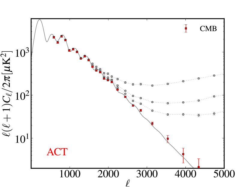
Figure 9 shows the estimated CMB bandpowers from the ACT-E and ACT-S spectra, co-added together and compared to the multi-frequency spectra. The bandpowers for each region are reported in Table 5. In this table we report the CMB spectra derived using the updated ‘v2’ multi-frequency spectra. Without assuming any cosmological model, the CMB bandpowers over the full angular range are remarkably consistent with the theoretical CDM model predicted by WMAP. The uncertainty on the bandpowers rises at scales smaller than , and the correlations between bandpowers increases.
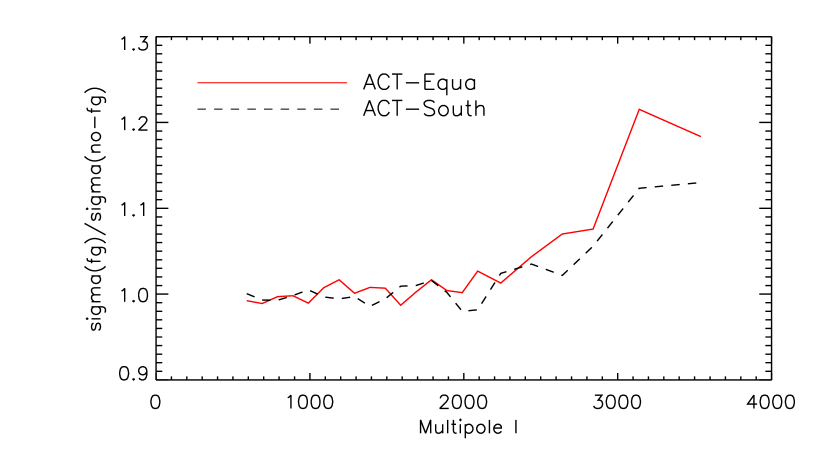
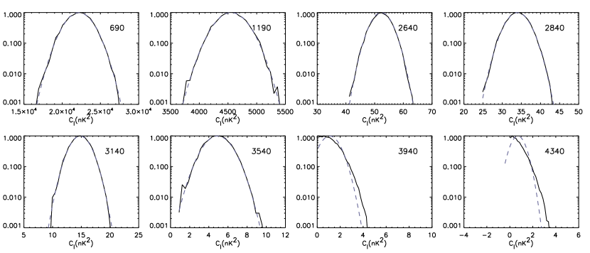
Figure 10 shows the effect of marginalization on the bandpower errors, using the ratio between the marginalized errors and the unmarginalized errors for a fixed secondary model. It is clear that by measuring the spectrum at multiple frequencies, the CMB can be successfully separated from secondary contamination out to scales . At scales there is little error inflation due to foreground uncertainty, and the errors are inflated by 20% (15%) by for the ACT-E (ACT-S) spectra. The marginalized distributions for the CMB bandpowers are well approximated by Gaussians for multipoles to band-center for ACT, as shown in the Appendix.
We compare the secondary parameters recovered in this model-independent sampling to the case where CDM is assumed. This comparison is shown in the Appendix; the parameters are consistent, with about a shift in the estimated kSZ power. We find that the CMB bandpowers are not strongly correlated with the secondary parameters until scales well into the Silk damping tail at ; a dominant correlation is then with the kSZ power due to its blackbody frequency dependence, and a smaller kSZ power – compensated by larger primary CMB power – is allowed when the CDM assumption is relaxed. The CMB bandpower covariance matrix conserves this correlation information.
| K2) | |||
|---|---|---|---|
| ACT-E | ACT-S | Coaddbbfootnotemark: | |
| 590 | |||
| 690 | |||
| 790 | |||
| 890 | |||
| 990 | |||
| 1090 | |||
| 1190 | |||
| 1290 | |||
| 1390 | |||
| 1490 | |||
| 1590 | |||
| 1690 | |||
| 1790 | |||
| 1890 | |||
| 1990 | |||
| 2090 | |||
| 2240 | |||
| 2440 | |||
| 2640 | |||
| 2840 | |||
| 3140 | |||
| 3540 | |||
| 11footnotetext: To compute a likelihood using these data, ACT-E and ACT-S should be used with the covariance matrix and bandpower window functions provided on LAMBDA. 22footnotetext: This coadds the ACT-E and ACT-S CMB bandpowers for plotting purposes. | |||
5.3. The CMB-only likelihood
We construct the CMB-only likelihood from the angular range where the CMB bandpowers are Gaussian, conservatively choosing . We do not use the bandpowers as they are increasingly non-Gaussian, due to the foreground marginalization, and are more strongly correlated with foreground parameters. The likelihood is given by
| (26) |
Here
| (27) |
where and are the marginalized mean and covariance matrix for the bandpowers, and is the lensed CMB spectrum generated from e.g., CAMB. We use 21 bandpowers for ACT-E and ACT-S in the range . A single calibration parameter for each region is marginalized over analytically, following Bridle et al. (2002). The prescription for using this likelihood is simple, as no extra nuisance parameters are needed.
To test the performance of this compressed likelihood, results are compared using the full multi-frequency likelihood, and the CMB-only likelihood. Cosmological parameters are estimated for the restricted CDM 6-parameter model, and a set of more extended models that probe the damping tail and peak shapes, including the running of the spectral index, the number of relativistic degrees of freedom , the lensing amplitude , and the variation in fine structure constant, . Parameter constraints using both likelihoods agree to , and are reported in Sievers et al. (2013). We conclude that this is an efficient alternative to the full likelihood for the typical extensions considered in cosmological analyses, although the full likelihood may give more optimal results for unusual models with features far into the damping tail.
6. Summary
In this paper we have presented a likelihood formalism to describe the ACT multi-frequency power spectra that includes contributions from SZ and foreground components in addition to the lensed CMB. We model the data including four late-time astrophysical components: thermal and kinetic SZ, emission from CIB galaxies, and emission from radio galaxies.
We have quantified these components using seven power spectra, splitting the CIB into a Poisson and clustered part, and including power from the cross-correlation between tSZ emission from clusters, and emission from CIB galaxies that also trace the large scale structure. Rather than a minimal model with the fewest parameters, we have sought a model that includes our uncertainties with priors describing our knowledge from additional observations. For example, while the data do not demand that we include the tSZ-CIB correlation, we are motivated to include it to avoid placing unphysically strong limits on the kSZ power.
Modeling these astrophysical components allows us to probe the primordial CMB fluctuations down to an angular resolution of 4’ using ACT. We have used the model to extract an estimate of the primordial CMB spectrum well into the Silk damping tail, marginalizing over the foreground uncertainty. This produces a simplified compressed likelihood for use in cosmological parameter estimation.
We find that data observed by the South Pole Telescope give results consistent with ACT, accounting for the different removal of radio point sources, and different degree of contamination by Galactic cirrus. SPT and ACT have very different instrument design and scan strategies, and their observations on the sky have limited overlap. The excellent agreement between the datasets is not only an important cross-check but is another demonstration of cosmic homogeneity.
References
- Addison et al. (2012a) Addison, G. E., Dunkley, J., & Bond, J. R. 2012a, ArXiv e-prints, 1210.6697
- Addison et al. (2012b) Addison, G. E. et al. 2012b, ApJ, 752, 120, 1108.4614
- Addison et al. (2012c) Addison, G. E., Dunkley, J., & Spergel, D. N. 2012c, MNRAS, 427, 1741, 1204.5927
- Battaglia et al. (2012a) Battaglia, N., Bond, J. R., Pfrommer, C., & Sievers, J. L. 2012a, ApJ, 758, 75, 1109.3711
- Battaglia et al. (2010) Battaglia, N., Bond, J. R., Pfrommer, C., Sievers, J. L., & Sijacki, D. 2010, ApJ, 725, 91, 1003.4256
- Battaglia et al. (2012b) Battaglia, N., Natarajan, A., Trac, H., Cen, R., & Loeb, A. 2012b, ArXiv e-prints, 1211.2832
- Bode et al. (2012) Bode, P., Ostriker, J. P., Cen, R., & Trac, H. 2012, ArXiv e-prints, 1204.1762
- Bond et al. (2004) Bond, J. R., Contaldi, C., Lewis, A., & Pogosyan, D. 2004, International Journal of Theoretical Physics, 43, 599, arXiv:astro-ph/0406195
- Bond et al. (2003) Bond, J. R., Contaldi, C. R., & Pogosyan, D. 2003, Phil. Trans. Roy. Soc. Lond., A361, 2435, astro-ph/0310735
- Bond et al. (2000) Bond, J. R., Jaffe, A. H., & Knox, L. 2000, ApJ, 533, 19, astro-ph/9808264
- Bridle et al. (2002) Bridle, S. L., Crittenden, R., Melchiorri, A., Hobson, M. P., Kneissl, R., & Lasenby, A. N. 2002, MNRAS, 335, 1193
- Connolly et al. (2002) Connolly, A. J. et al. 2002, ApJ, 579, 42, arXiv:astro-ph/0107417
- Das et al. (2011) Das, S. et al. 2011, ApJ, 729, 62, 1009.0847
- Das et al. (2013) Das, S., et al. 2013, submitted
- Dunkley et al. (2005) Dunkley, J., Bucher, M., Ferreira, P. G., Moodley, K., & Skordis, C. 2005, MNRAS, 356, 925, arXiv:astro-ph/0405462
- Dunkley et al. (2011) Dunkley, J. et al. 2011, ApJ, 739, 52, 1009.0866
- Dunkley et al. (2009) ——. 2009, ApJS, 180, 306, 0803.0586
- Dünner et al. (2012) Dünner, R. et al. 2012, ArXiv e-prints, 1208.0050
- Efstathiou & Migliaccio (2012) Efstathiou, G., & Migliaccio, M. 2012, MNRAS, 3051, 1106.3208
- Eriksen et al. (2004) Eriksen, H. K., Hansen, F. K., Banday, A. J., Górski, K. M., & Lilje, P. B. 2004, ApJ, 605, 14
- Finkbeiner et al. (1999) Finkbeiner, D. P., Davis, M., & Schlegel, D. J. 1999, ApJ, 524, 867, astro-ph/9905128
- Fowler et al. (2010) Fowler, J. W. et al. 2010, ApJ, 722, 1148, 1001.2934
- Giavalisco et al. (1998) Giavalisco, M., Steidel, C. C., Adelberger, K. L., Dickinson, M. E., Pettini, M., & Kellogg, M. 1998, ApJ, 503, 543, arXiv:astro-ph/9802318
- Gispert et al. (2000) Gispert, R., Lagache, G., & Puget, J. L. 2000, A&A, 360, 1, arXiv:astro-ph/0005554
- Gold et al. (2011) Gold, B. et al. 2011, ApJS, 192, 15, 1001.4555
- Gralla et al. (2013) Gralla, M., et al. 2013, in preparation
- Gruzinov & Hu (1998) Gruzinov, A., & Hu, W. 1998, ApJ, 508, 435, arXiv:astro-ph/9803188
- Hajian et al. (2011) Hajian, A. et al. 2011, ApJ, 740, 86, 1009.0777
- Hajian et al. (2012) ——. 2012, ApJ, 744, 40, 1101.1517
- Hall et al. (2010) Hall, N. R. et al. 2010, ApJ, 718, 632, 0912.4315
- Hauser et al. (1998) Hauser, M. G. et al. 1998, ApJ, 508, 25, arXiv:astro-ph/9806167
- Hinshaw et al. (2003) Hinshaw, G. et al. 2003, ApJS, 148, 135
- Iliev et al. (2007) Iliev, I. T., Mellema, G., Shapiro, P. R., & Pen, U.-L. 2007, MNRAS, 376, 534, arXiv:astro-ph/0607517
- Itoh et al. (1998) Itoh, N., Kohyama, Y., & Nozawa, S. 1998, ApJ, 502, 7, arXiv:astro-ph/9712289
- Jewell et al. (2004) Jewell, J., Levin, S., & Anderson, C. H. 2004, ApJ, 609, 1, arXiv:astro-ph/0209560
- Keisler et al. (2011) Keisler, R. et al. 2011, ApJ, 743, 28, 1105.3182
- Komatsu & Seljak (2002) Komatsu, E., & Seljak, U. 2002, MNRAS, 336, 1256
- Komatsu et al. (2011) Komatsu, E. et al. 2011, ApJS, 192, 18, 1001.4538
- Lagache et al. (2007) Lagache, G., Bavouzet, N., Fernandez-Conde, N., Ponthieu, N., Rodet, T., Dole, H., Miville-Deschênes, M.-A., & Puget, J.-L. 2007, ApJ, 665, L89, 0707.2443
- Larson et al. (2011) Larson, D. et al. 2011, ApJS, 192, 16, 1001.4635
- Lewis & Bridle (2002) Lewis, A., & Bridle, S. 2002, Phys. Rev. D, 66, 103511
- Lewis et al. (2000) Lewis, A., Challinor, A., & Lasenby, A. 2000, ApJ, 538, 473
- Lueker et al. (2010) Lueker, M. et al. 2010, ApJ, 719, 1045, 0912.4317
- Marriage et al. (2011) Marriage, T. A. et al. 2011, ApJ, 731, 100, 1007.5256
- McQuinn et al. (2005) McQuinn, M., Furlanetto, S. R., Hernquist, L., Zahn, O., & Zaldarriaga, M. 2005, ApJ, 630, 643, arXiv:astro-ph/0504189
- Mesinger et al. (2012) Mesinger, A., McQuinn, M., & Spergel, D. N. 2012, MNRAS, 422, 1403, 1112.1820
- Miville-Deschênes & Lagache (2005) Miville-Deschênes, M.-A., & Lagache, G. 2005, ApJS, 157, 302, arXiv:astro-ph/0412216
- Nolta et al. (2009) Nolta, M. R. et al. 2009, ApJS, 180, 296, 0803.0593
- Ostriker & Vishniac (1986) Ostriker, J. P., & Vishniac, E. T. 1986, ApJ, 306, L51
- Planck Collaboration I et al. (2011) Planck Collaboration I et al. 2011, A&A, 536, A1, 1101.2022
- Planck Collaboration XIX et al. (2011) Planck Collaboration XIX et al. 2011, A&A, 536, A19, 1101.2029
- Planck Collaboration XVIII et al. (2011) Planck Collaboration XVIII et al. 2011, A&A, 536, A18, 1101.2028
- Puget et al. (1996) Puget, J.-L., Abergel, A., Bernard, J.-P., Boulanger, F., Burton, W. B., Desert, F.-X., & Hartmann, D. 1996, A&A, 308, L5
- Reichardt et al. (2012) Reichardt, C. L. et al. 2012, ApJ, 755, 70, 1111.0932
- Sehgal et al. (2010) Sehgal, N. et al. 2010, ApJ, 709, 920, arXiv:0908.0540
- Sharp et al. (2010) Sharp, M. K. et al. 2010, ApJ, 713, 82, 0901.4342
- Shaw et al. (2010) Shaw, L. D., Nagai, D., Bhattacharya, S., & Lau, E. T. 2010, ApJ, 725, 1452, 1006.1945
- Shaw et al. (2012) Shaw, L. D., Rudd, D. H., & Nagai, D. 2012, ApJ, 756, 15, 1109.0553
- Shaw et al. (2009) Shaw, L. D., Zahn, O., Holder, G. P., & Doré, O. 2009, ApJ, 702, 368, 0903.5322
- Shirokoff et al. (2011) Shirokoff, E. et al. 2011, ApJ, 736, 61, 1012.4788
- Sievers et al. (2013) Sievers, J., et al. 2013, submitted
- Sievers et al. (2003) Sievers, J. L. et al. 2003, ApJ, 591, 599
- Sievers et al. (2009) ——. 2009, ArXiv e-prints, 0901.4540
- Silk (1968) Silk, J. 1968, ApJ, 151, 459
- Spergel et al. (2003) Spergel, D. N. et al. 2003, ApJS, 148, 175
- Story et al. (2012) Story, K. T. et al. 2012, ArXiv e-prints, 1210.7231
- Sunyaev & Zel’dovich (1970) Sunyaev, R. A., & Zel’dovich, Y. B. 1970, 7, 3
- Swetz et al. (2011) Swetz, D. S. et al. 2011, ApJS, 194, 41, 1007.0290
- Trac et al. (2011) Trac, H., Bode, P., & Ostriker, J. P. 2011, ApJ, 727, 94, 1006.2828
- Vieira et al. (2010) Vieira, J. D. et al. 2010, ApJ, 719, 763, 0912.2338
- Viero et al. (2009) Viero, M. P. et al. 2009, ApJ, 707, 1766, 0904.1200
- Wandelt et al. (2004) Wandelt, B. D., Larson, D. L., & Lakshminarayanan, A. 2004, Phys. Rev. D, 70, 083511, arXiv:astro-ph/0310080
- Zahn et al. (2012) Zahn, O. et al. 2012, ApJ, 756, 65, 1111.6386