Decays $B_{s}\rightarrow J/\psi+\eta$ and $B_{s}\rightarrow J/\psi+\eta^{\prime}$ in the framework of covariant quark model

Abstract

The covariant quark model represents an appropriate theoretical framework to describe the recent results on $B_{s}\rightarrow J/\psi+\eta$ and $B_{s}\rightarrow J/\psi+\eta^{\prime}$ decays from the Belle and LHCb collaborations. In this article we present the main features of the covariant quark model together with details on some of its aspects and methods, which we consider to be important. Further we apply the model specifically to the studied decay processes and give numerical results on decay widths as they follow from the model. We conclude that the model, with most of its parameters previously fixed from different processes, is able to incorporate the new experimental measurements. In particular, we found that the ratio of the branching fractions of the decays $B_{s}$ into $J/\psi+\eta^{\prime}$ and $J/\psi+\eta$ is equal to $R\approx 0.86$, in agreement with the data reported by Belle and LHCb collaborations.

I Introduction

The low energy region of quantum chromodynamics (QCD) is an interesting and challenging area of investigation nowadays. On one hand many accurate data exists in this domain, especially results from hadron spectroscopy and hadron decays, which might give a handle to understanding the quark dynamics inside hadrons. Presently the precision and the amount of these data continuously increases thanks to ongoing high-energy experiments and heavy-quark factories. On the other hand theoretical predictions encounter difficulties: since with decreasing energy the coupling constant increases, the perturbative approach (pQCD) looses its applicability and cannot provide valid results. Also lattice calculations are generally seen as not yet enough developed and precise to be considered as a well established low-energy solution of the QCD which would satisfactory explain its numerous features. Undoubtedly however, some theoretical description of hadron dynamics is needed at least for a correct description of physic and background measured in particle detectors. One thus has to rely on a model-dependent approach.

In the wake of the recent measurement of the branching fractions of $B_{s}$ meson decays into $J/\psi+\eta$ and $J/\psi+\eta^{\prime}$ made by Belle Li et al. (2012) and LHCb Aaij et al. (2013) collaborations, we perform the analysis of the above processes in the framework of the covariant quark model.

Theoretical facets of these decays in the context of exploring CP violation have been discussed in the papers Refs. Skands (2001); Colangelo et al. (2011); Di Donato et al. (2012); Fleischer et al. (2011). Two points are important in analyzing: $SU_{f}(3)$ breaking and $\eta-\eta^{\prime}$ mixing. There are attempts to include in addition the admixture of glueball in the $\eta-\eta^{\prime}$ mixing, see i.e. Liu et al. (2012).

The covariant quark model Branz et al. (2010) is an ambitious model with many appealing features. Its Lagrangian-based formulation leads to a full Lorentz invariance and, in the limit of large number of hadrons, it has only one free parameter per hadron. A distinctive feature of this approach is that the multiquark states, such as baryons (three quarks), tetraquarks (four quarks), etc., can be considered and described as rigorously as the simplest quark-antiquark systems (mesons). The model has wide application spectra and was already successfully used to describe different types of heavy hadron decays and other hadron-related observables. The last applications have been done for studying the properties of the $B_{s}$ meson Ivanov et al. (2012), the light baryons Gutsche et al. (2012), the heavy $\Lambda_{b}$ baryon Gutsche et al. (2013) and tetraquarks Dubnička et al. (2010, 2011). The results are reviewed in Ref. Ivanov (2013).

In Sec. II we briefly discuss the basic features of our approach. In Sec. III we give more details on the compositeness condition, the infrared confinement and calculational techniques. The calculation of the matrix elements of the decays $B_{s}\rightarrow J/\psi+\eta$ and $B_{s}\rightarrow J/\psi+\eta^{\prime}$ is performed in Sec. IV. In Sec. V the calculated results are reported and comparison with available experimental data is given. Finally, in Sec. VI we summarize our findings.

II Covariant quark model

The interaction Lagrangian (density) of the model

$$\mathrm{\mathcal{L}_{int}=g_{H}H\left(x\right)\cdot J_{H}\left(x\right)+H.c.}$$ (1)

is constructed from the hadron field $\mathrm{H\left(x\right)}$ and the quark current. The latter is in case of mesons written as

$$\mathrm{J_{M}\left(x\right)} \mathrm{=} \mathrm{\int dx_{1}\int dx_{2}F_{M}\left(x;x_{1},x_{2}\right)\times\bar{q}_{2}^{a}\left(x_{2}\right)\Gamma_{M}q_{1}^{a}\left(x_{1}\right)}$$ (2)

and makes appear that, within the model, the interaction is mediated only by the quarks and the gluons are absent. The form of the vertex function $\mathrm{F_{M}}$ is chosen such as to reflect the intuitive expectations about relative quark-hadron positions

$$\mathrm{F_{M}\left(x;x_{1},x_{2}\right)} \mathrm{=} \mathrm{\delta^{\left(4\right)}\left(x-w_{1}x_{1}-w_{2}x_{2}\right)\times\Phi_{M}\left[\left(x_{1}-x_{2}\right)^{2}\right],}$$ (3)

where we require $\mathrm{w_{1}+w_{2}=1}$. We actually adopt the most natural choice

$$\mathrm{w_{i}=\frac{m_{i}}{m_{1}+m_{2}},\>i=1,2}$$ (4)

where the barycenter of the hadron is identified with the barycenter of the quark system. The interaction strength $\mathrm{\Phi_{M}\left[\left(x_{1}-x_{2}\right)^{2}\right]}$ is assumed to have a Gaussian form which is in the momentum representation written as

$$\mathrm{\widetilde{\Phi}_{M}\left(-p^{2}\right)=\exp\left(\frac{p^{2}}{\Lambda_{M}^{2}}\right)}.$$ (5)

Here $\mathrm{\Lambda_{M}}$ is a hadron-related size parameter which is regarded as a free parameter of the model. Additional free parameters are the quark masses

$$\mathrm{m_{u,d}=0.235\>GeV,} \mathrm{m_{s}=0.424\>GeV,}$$

$$\mathrm{m_{c}=2.16\>GeV,} \mathrm{m_{b}=5.09\>GeV}$$ (6)

and a universal cut-off parameter $\mathrm{\lambda_{cut-off}}$, which is commented on in more details later in this text. The numerical values of these parameters as well as of size parameters for several hadrons were fixed by fitting the model to measurement data of simple quantities, such as leptonic decay constants and electromagnetic decay widths Ivanov et al. (2012). The value of the size parameter for $B_{s}$ meson is $\mathrm{\Lambda_{B_{s}}=1.95\>GeV}$. The model thus has in total $\mathrm{N_{H}+5}$ parameters: for each of $\mathrm{N_{H}}$ hadrons one $\Lambda$ parameter, four quark masses and one universal cut-off. The coupling constants $\mathrm{g_{M}}$ can be related to these parameters using the so-called compositeness condition, which is discussed in the following section.

III Compositeness condition, calculation methods and infrared confinement

In this section we give more details about some issues related to the model. As announced previously, one of them is the compositeness condition.

The quark fields as well as the hadron field enter the interaction Lagrangian of the model (1) as elementary although, in nature, the hadrons are compound of quarks. An effort was made in theoretical physics to find an appropriate description of composite particles. The authors of the references Salam (1962); Weinberg (1963) argue, that the hadron fields renormalization constant $\mathrm{Z_{H}^{\frac{1}{2}}}$ can be interpreted as the matrix element between the physical state and the corresponding bare state. The case $\mathrm{Z_{H}=0}$ thus corresponds to a state not containing the bare state and can be therefore properly interpreted as a bound state. This idea was used and introduced into the covariant quark model Efimov and Ivanov (1993, 1989). The renormalization constant is expressed through the derivative of the meson mass operator and takes the form

$$\mathrm{Z_{M}=1-\frac{3g_{M}^{2}}{4\pi^{2}}\tilde{\Pi}_{M}^{{}^{\prime}}\left(m_{M}^{2}\right)=0}.$$ (7)

The coupling constants are in this way eliminated as free parameters. This not only gives the model more predictive power but also helps to stabilize model predictions over wide spectra of hadron data. The first step in calculation of physical observables is thus the determination of couplings $\mathrm{g_{M}}$ of participating hadrons.

In the case of the pseudoscalar and vector mesons the derivative of the meson mass operator can be calculated in the following way

$$\mathrm{\widetilde{\Pi}^{\prime}_{P}(p^{2})} \mathrm{=} \mathrm{\frac{1}{2p^{2}}\,p^{\alpha}\frac{d}{dp^{\alpha}}\,\int\!\!\frac{d^{4}k}{4\pi^{2}i}\,\widetilde{\Phi}_{P}^{2}(-k^{2})\times{\rm tr}\biggl{[}\gamma^{5}S_{1}(k+w_{1}p)\gamma^{5}S_{2}(k-w_{2}p)\biggr{]}}\mathrm{}$$

$$\mathrm{=} \mathrm{\frac{1}{2p^{2}}\,\int\!\!\frac{d^{4}k}{4\pi^{2}i}\,\widetilde{\Phi}_{P}^{2}(-k^{2})\times\Big{\{}w_{1}\,{\rm tr}\biggl{[}\gamma^{5}S_{1}(k+w_{1}p)\!\not\!pS_{1}(k+w_{1}p)\gamma^{5}S_{2}(k-w_{2}p)\biggr{]}}$$

$$\mathrm{-w_{2}\,{\rm tr}\biggl{[}\gamma^{5}S_{1}(k+w_{1}p)\gamma^{5}S_{2}(k-w_{2}p)\!\not\!p\,S_{2}(k-w_{2}p)\biggr{]}\Big{\}},}$$

$$\mathrm{\widetilde{\Pi}^{\prime}_{V}(p^{2})} \mathrm{=} \mathrm{\frac{1}{3}\left(g_{\mu\nu}-\frac{p_{\mu}p_{\nu}}{p^{2}}\right)\times\frac{1}{2p^{2}}\,p^{\alpha}\frac{d}{dp^{\alpha}}\,\int\!\!\frac{d^{4}k}{4\pi^{2}i}\,\widetilde{\Phi}_{V}^{2}(-k^{2})\times{\rm tr}\biggl{[}\gamma^{\mu}S_{1}(k+w_{1}p)\gamma^{\nu}S_{2}(k-w_{2}p)\biggr{]}}$$ (8)

$$\mathrm{=} \mathrm{\frac{1}{3}\left(g_{\mu\nu}-\frac{p_{\mu}p_{\nu}}{p^{2}}\right)\frac{1}{2p^{2}}\,\int\!\!\frac{d^{4}k}{4\pi^{2}i}\times\widetilde{\Phi}_{V}^{2}(-k^{2})}$$

$$\mathrm{\times\Big{\{}w_{1}\,{\rm tr}\biggl{[}\gamma^{\mu}S_{1}(k+w_{1}p)\not\!p\>S_{1}(k+w_{1}p)\gamma^{\nu}S_{2}(k-w_{2}p)\biggr{]}}$$

$$\mathrm{-w_{2}\,{\rm tr}\biggl{[}\gamma^{\mu}S_{1}(k+w_{1}p)\gamma^{\nu}S_{2}(k-w_{2}p)\!\not\!p\,S_{2}(k-w_{2}p)\biggr{]}\Big{\}},}$$

where $\mathrm{\widetilde{\Phi}_{M}\left(-k^{2}\right)}$ is the Fourier transform of the vertex function $\mathrm{\Phi_{M}\left[\left(x_{1}-x_{2}\right)^{2}\right]}$ and $\mathrm{S_{i}(k)}$ is the quark propagator. We have used free fermion propagators for the quarks given by

$$\mathrm{S_{q}(k)=\frac{1}{m_{q}-\not\!k}}$$ (9)

with an effective constituent quark mass $\mathrm{m_{q}}$.

In computation of Feynman diagrams we use, in the momentum space, the Schwinger representation of the quark propagator

$$\mathrm{S_{q}(k)} \mathrm{=} \mathrm{\frac{m_{q}+\not\!k}{m_{q}^{2}-k^{2}}}$$ (10)

$$\mathrm{=} \mathrm{\left(m_{q}+\not\!k\right)\intop_{0}^{\infty}d\alpha\>e^{-\alpha\left(m^{2}-k^{2}\right)}}$$

The general form of a resulting Feynman diagrams is

$$\mathrm{\Pi\left(p_{1},\ldots,p_{m}\right)=\intop_{0}^{\infty}d^{n}\alpha\int\left[d^{4}k\right]^{\ell}\Phi\times\exp\left\{-\sum_{i=1}^{n}\alpha_{i}\left[m_{i}^{2}-\left(K_{i}+P_{i}\right)^{2}\right]\right\},}$$ (11)

where $\mathrm{K_{i}}$ represents a linear combination of loop momenta, $\mathrm{P_{i}}$ stands for a linear combination of external momenta and $\mathrm{\Phi}$ refers to the numerator product of propagators and vertex functions. The evaluation of these expressions can be much simplified if done in a smart way. One can use two operator identities, of which the first one

$$\mathrm{\int d^{4}k\>P\left(k\right)e^{2kr}} \mathrm{=}\mathrm{\int d^{4}k\>P\left(\frac{1}{2}\frac{\partial}{\partial r}\right)e^{2kr}}$$

$$\mathrm{=}\mathrm{P\left(\frac{1}{2}\frac{\partial}{\partial r}\right)\int d^{4}k\>e^{2kr}}$$ (12)

is suited for en elegant loop momenta integration. The second one

$$\mathrm{\intop_{0}^{\infty}d^{n}\alpha\>P\left(\frac{1}{2}\frac{\partial}{\partial r}\right)e^{-\frac{r^{2}}{a}}=\intop_{0}^{\infty}d^{n}\alpha\>e^{-\frac{r^{2}}{a}}P\left(\frac{1}{2}\frac{\partial}{\partial r}-\frac{r}{a}\right)\mathds{1},}$$ (13)

where $\mathrm{r=r\left(\alpha_{i}\right)}$ and $\mathrm{a=a\left(\Lambda_{M},\alpha_{i}\right)}$, simplifies the computation following the trace evaluation: the polynomial in the derivative operator which results from the trace can be applied to an identity, instead being applied to a more complicated exponential function.

The last point which remains to be discussed is the cut-off we apply in the integration over the Schwinger parameters. This integration is multidimensional with the limits from $0$ to $+\infty$. In order to arrive to a single cut-off parameter we firstly transform the integral over an infinite space into an integral over a simplex convoluted with only one-dimensional improper integral. For that purpose we use the $\delta$-function form of the identity

$$\mathrm{\mathds{1}=\intop_{0}^{\infty}dt\>\delta\left(t-\sum_{i=1}^{n}\alpha_{i}\right)}$$ (14)

from which follows

$$\Pi=\intop_{0}^{\infty}dt\>t^{n-1}\intop_{0}^{1}d^{n}\alpha\>\delta\left(t-\sum_{i=1}^{n}\alpha_{i}\right)\times W\left(t\alpha_{1},\ldots,t\alpha_{1}\right),$$ (15)

where $W$ represents the integrand of Schwinger parameters. The cut-off $\lambda$ is then introduced in a natural way

$$\intop_{0}^{\infty}dt\>t^{n-1}\ldots\rightarrow\intop_{0}^{1/\lambda^{2}}dt\>t^{n-1}\ldots.$$ (16)

Such a cut-off makes the integral to be an analytic function without any singularities. In this way all potential thresholds in the quark loop diagrams are removed together with corresponding branch points Branz et al. (2010). Within covariant quark model the cut-off parameter is universal for all processes and its value, as obtained from a fit to data, is

$$\mathrm{\lambda_{cut-off}=0.181\>GeV.}$$ (17)

The integrals are computed numerically.

IV Decays $B_{s}\rightarrow J/\psi+\eta$ and $B_{s}\rightarrow J/\psi+\eta^{\prime}$

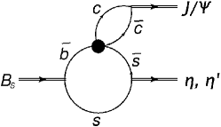
(a)

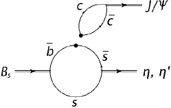
(b)

Figure 1: a) Diagram of $B_{s}\rightarrow J/\psi+\eta^{\left(\prime\right)}$ decay. b) Factorization of the diagram.

The diagram of the $B_{s}\rightarrow J/\psi+\eta^{\left(\prime\right)}$ decay is shown in Fig. 1a. The $\eta$ and $\eta^{\prime}$ particles are mixture of the light and the $s$-quark component. In the approximation $m_{u}=m_{d}\equiv m_{q}$ one can write their quark content as

$$\mathrm{\mathrm{\eta}} \mathrm{\mathrm{:}} \mathrm{\mathrm{-\frac{1}{\sqrt{2}}\sin\delta\left(u\bar{u}+d\bar{d}\right)-\cos\delta\left(s\bar{s}\right)}}$$ (18)

$$\mathrm{\mathrm{=-\sin\delta\left(q\bar{q}\right)-\cos\delta\left(s\bar{s}\right),}}$$

$$\mathrm{\mathrm{\eta^{\prime}}} \mathrm{:} \frac{1}{\sqrt{2}}\mathrm{\cos\delta\left(u\bar{u}+d\bar{d}\right)-\sin\delta\left(s\bar{s}\right)}$$ (19)

$$\mathrm{=\cos\delta\left(q\bar{q}\right)-\sin\delta\left(s\bar{s}\right),}$$

with

$$\mathrm{q\bar{q}=\frac{1}{\sqrt{2}}\left(u\bar{u}+d\bar{d}\right)}$$ (20)

and

$$\mathrm{\delta} \mathrm{=} \mathrm{\theta_{P}-\theta_{I},}$$ (21)

$$\mathrm{\theta_{I}=\arctan\frac{1}{\sqrt{2}}\approx 35.26^{\circ},}$$

$$\theta_{P}\approx-13.34^{\circ}.$$

The value of the pseudoscalar angle $\theta_{P}$ is deduced from the Ref. Ambrosino et al. (2007), where however a different convention is used for the mixing angle $\mathrm{\varphi_{P}}$. It can be related to ours by $\mathrm{\delta=\varphi_{P}-\pi/2}$.

We describe the decay only through the dominant $s$-quark contribution to the $\eta^{\left(\prime\right)}$ meson since the light quark one results from higher-order diagrams. The quark-hadron interaction is described by the Lagrangians from the Section II (see Appendix A.1) and we use an effective theory with four-quark interaction to describe the production of the $J/\psi$ particle. The Lagrangian of this interaction is written as

$$\mathrm{\mathcal{L}_{eff}=\frac{G_{F}}{\sqrt{2}}V_{cb}V_{cs}^{*}\sum_{i}C_{i}Q_{i},}$$ (22)

where $\mathrm{G_{F}}$ is the Fermi Coupling Constant, $\mathrm{V_{xy}}$ refers to the elements of the CKM matrix, $\mathrm{C_{i}}$ are the Wilson coefficients (Ref. Altmannshofer et al. (2009)) and $Q_{i}$ are operators listed in Appendix A.2. To each component of both $\eta$ and $\eta^{\prime}$ particles we associate a size parameter. So, in general, the description requires four free parameters $\mathrm{\Lambda_{\eta}^{q\bar{q}}}$, $\mathrm{\Lambda_{\eta}^{s\bar{s}}}$ , $\mathrm{\Lambda_{\eta^{\prime}}^{q\bar{q}}}$ and $\mathrm{\Lambda_{\eta^{\prime}}^{s\bar{s}}}$. We consider the mixing angle $\mathrm{\delta}$ as fixed although, in principle, it also might be varied to determine its most suited value within the covariant quark model. As a model-independent parameter it can be compared to other models and to data.

An important simplification in calculations comes from the evaluation of the $\mathrm{Q_{i}}$ operator matrix elements. In can be shown that the expression factorizes into a part that corresponds to the $\mathrm{B_{s}\rightarrow\eta^{\left(\prime\right)}}$ transition form factor and a part that is proportional to the decay constant of the $\mathrm{J/\psi}$ particle (Fig 1b and Appendix A.3).

It is readily seen from the Fig. 1b that only the strange quark component gives the contribution to the color-suppressed $B_{s}\rightarrow\eta^{\left(\prime\right)}$ decays. The invariant matrix element describing this decay is written as

$$\mathrm{M\left[B_{s}(p_{1})\to P_{s\bar{s}}(p_{2})+J/\psi(q)\right]=\frac{G_{F}}{\sqrt{2}}V_{cb}V_{cs}^{\dagger}C_{W}F_{+}^{B_{s}P_{s\bar{s}}}(q^{2})\,m_{J/\psi}f_{J/\psi}\,(p_{1}+p_{2})\cdot\epsilon_{J/\psi},}$$ (23)

where $\mathrm{q=p_{1}-p_{2}}$, $\mathrm{q\cdot\epsilon_{J/\psi}=0}$, $\mathrm{q^{2}=m_{J/\psi}^{2}}$ and the color factor $\mathrm{C_{W}}=\mathrm{C_{1}}+\xi\mathrm{C_{2}}+\mathrm{C_{3}}+\xi\mathrm{C_{4}}+\mathrm{C_{5}}+\xi\mathrm{C_{6}}$ with $\mathrm{\xi=1/N_{c}}$. The terms multiplied by the color factor $\mathrm{\xi}$ will be dropped in the numerical calculations according to the $\mathrm{1/N_{c}}$ expansion.

The leptonic decay constants of the pseudoscalar and vector mesons are defined by

$$\mathrm{N_{c}\,g_{P}\!\int\!\!\frac{d^{4}k}{(2\pi)^{4}i}\,\widetilde{\Phi}_{P}(-k^{2})\,{\rm tr}\biggl{[}O^{\,\mu}S_{1}(k+w_{1}p)\gamma^{5}S_{2}(k-w_{2}p)\biggr{]}} \mathrm{=} \mathrm{f_{P}p^{\mu},\quad p^{2}=m_{P}^{2},}$$

$$\mathrm{N_{c}\,g_{V}\!\int\!\!\frac{d^{4}k}{(2\pi)^{4}i}\,\widetilde{\Phi}_{V}(-k^{2})\,{\rm tr}\biggl{[}O^{\,\mu}S_{1}(k+w_{1}p)\not\!\epsilon_{V}S_{2}(k-w_{2}p)\biggr{]}} \mathrm{=} \mathrm{m_{V}f_{V}\epsilon_{V}^{\mu},\quad p^{2}=m_{V}^{2}.}$$ (24)

The form factors of the $\mathrm{P_{[\bar{q}_{3}q_{2}]}-P_{[\bar{q}_{1}q_{3}]}^{\,\prime}}$ transition are given by

$$\mathrm{\langle P_{[\bar{q}_{1}q_{3}]}^{\,\prime}(p_{2})\,|\,\bar{q}_{2}\,O^{\,\mu}\,q_{1}\,|P_{[\bar{q}_{3}q_{2}]}(p_{1})\rangle} \mathrm{=} \mathrm{N_{c}\,g_{P}\,g_{P^{\,{}^{\prime}}}\!\int\!\frac{d^{4}k}{(2\pi)^{4}i}\>\widetilde{\Phi}_{P}\Big{(}-(k+w_{13}p_{1})^{2}\Big{)}\,\widetilde{\Phi}_{P^{\,{}^{\prime}}}\Big{(}-(k+w_{23}p_{2})^{2}\Big{)}}$$ (25)

$$\qquad\mathrm{\times{\rm tr}\biggl{[}O^{\,\mu}\,S_{1}(k+p_{1})\,\gamma^{5}\,S_{3}(k)\,\gamma^{5}\,S_{2}(k+p_{2})\biggr{]}}$$

$$\mathrm{=} \mathrm{F_{+}(q^{2})\,P^{\,\mu}+F_{-}(q^{2})\,q^{\,\mu}}$$

where in addition to Eq. (4) we have introduced a two-subscript notation $\mathrm{w_{ij}=m_{j}/(m_{i}+m_{j})}$ such that $\mathrm{w_{ij}+w_{ji}=1}$. The calculation of the widths is straightforward. One has

$$\mathrm{\Gamma(B_{s}\to J/\psi+\eta)=\frac{G_{F}^{2}}{4\pi}|V_{cb}V_{cs}^{\dagger}|^{2}C_{W}^{2}\,f_{J/\psi}^{2}\,|\mathbf{q}_{\eta}|^{3}\cos^{2}\delta\left(F_{+}^{B_{s}\eta}(m_{J/\psi}^{2})\right)^{2},}$$

$$\mathrm{\Gamma(B_{s}\to J/\psi+\eta^{\prime})=\frac{G_{F}^{2}}{4\pi}|V_{cb}V_{cs}^{\dagger}|^{2}C_{W}^{2}\,f_{J/\psi}^{2}\,|\mathbf{q}_{\eta^{\prime}}|^{3}\sin^{2}\delta\left(F_{+}^{B_{s}\eta^{\prime}}(m_{J/\psi}^{2})\right)^{2},}$$ (26)

where $\mathrm{|{\mathbf{q}_{P}}|=\lambda^{1/2}(m_{B_{s}}^{2},m_{P}^{2},m_{J/\psi}^{2})/(2m_{B_{s}})}$ is the momentum of the outgoing particles in the rest frame of the decaying particle.

In addition to the Belle results, we need further data in order to over-constrain the model. We have chosen the following decays

$$\eta\rightarrow\gamma\gamma \varphi\rightarrow\eta\gamma$$

$$\eta^{\prime}\rightarrow\gamma\gamma \varphi\rightarrow\eta^{\prime}\gamma$$

$$\rho^{0}\rightarrow\eta\gamma B_{d}\rightarrow J/\psi+\eta$$

$$\omega\rightarrow\eta\gamma B_{d}\rightarrow J/\psi+\eta^{\prime}$$

$$\eta^{\prime}\rightarrow\omega\gamma$$ (27)

These processes have already been previously described by the covariant quark model Branz et al. (2010) and can be straightforwardly included into a global fit.

V Results and discussion

Observable	Covariant	Experiment		Other models
	quark model			Münz Munz et al. (1994)	Becchi Becchi and Morpurgo (1965)	Jaus Jaus (1991)
$\Gamma_{\eta\rightarrow\gamma\gamma}$	$\mathrm{0.380\>keV}$	$\mathrm{0.511\pm 0.028\>keV}$	Babusci et al. (2013)	$\mathrm{0.440\>keV}$	-	$\mathrm{0.485\>keV}$
$\mathrm{\Gamma_{\eta^{\prime}\rightarrow\gamma\gamma}}$	$\mathrm{3.74\>keV}$	$\mathrm{4.34\pm 0.14\>keV}$	Beringer et al. (2012)	$\mathrm{2.90\>keV}$	-	$\mathrm{2.90\>keV}$
$\mathrm{\Gamma_{\rho^{0}\rightarrow\eta\gamma}}$	$\mathrm{53.07\>keV}$	$\mathrm{44.73\pm 2.99\>keV}$	Beringer et al. (2012)	-	$\mathrm{44\>keV}$	$\mathrm{59\>keV}$
$\mathrm{\Gamma_{\omega\rightarrow\eta\gamma}}$	$\mathrm{6.21\>keV}$	$\mathrm{3.91\pm 0.34\>keV}$	Beringer et al. (2012)	-	$\mathrm{6.4\>keV}$	$\mathrm{8.7\>keV}$
$\mathrm{\Gamma_{\eta^{\prime}\rightarrow\omega\gamma}}$	$\mathrm{9.49\>keV}$	$\mathrm{5.47\pm 0.63\>keV}$	Beringer et al. (2012)	-	-	$\mathrm{4.8\>keV}$
$\mathrm{\Gamma_{\varphi\rightarrow\eta\gamma}}$	$\mathrm{42.59\>keV}$	$\mathrm{58.90\pm 2.45\>keV}$	Beringer et al. (2012)	-	$\mathrm{304\>keV}$	$\mathrm{55.3\>keV}$
$\mathrm{\Gamma_{\varphi\rightarrow\eta^{\prime}\gamma}}$	$\mathrm{0.276\>keV}$	$\mathrm{0.281\pm 0.015\>keV}$	Beringer et al. (2012)	-	-	$\mathrm{0.57\>keV}$
$\mathrm{{\cal B}_{B_{d}\rightarrow J/\psi+\eta}}$	$\mathrm{16.5\times 10^{-6}}$	$\mathrm{\left(12.3\pm 1.9\right)\times 10^{-6}}$	Chang et al. (2012)	-	-	-
$\mathrm{{\cal B}_{B_{d}\rightarrow J/\psi+\eta^{\prime}}}$	$\mathrm{12.2\times 10^{-6}}$	$\mathrm{<7.4\times 10^{-6}}$	Chang et al. (2012)	-	-	-
$\mathrm{{\cal B}_{B_{s}\rightarrow J/\psi+\eta}}$	$\mathrm{4.67\times 10^{-4}}$	$\mathrm{\left(5.10\pm 1.12\right)\times 10^{-4}}$	Li et al. (2012)	-	-	-
$\mathrm{{\cal B}_{B_{s}\rightarrow J/\psi+\eta^{\prime}}}$	$\mathrm{4.04\times 10^{-4}}$	$\mathrm{\left(3.71\pm 0.95\right)\times 10^{-4}}$	Li et al. (2012)	-	-	-

Table 1: Decay widths and branching fractions for selected processes: model predictions and data.

The optimal model parameters (in $\mathrm{GeV}$)

$$\mathrm{\Lambda_{\eta}^{q\bar{q}}=0.881,\quad\Lambda_{\eta}^{s\bar{s}}=1.973}$$

$$\mathrm{\Lambda_{\eta^{\prime}}^{q\bar{q}}=0.257,\quad\Lambda_{\eta^{\prime}}^{s\bar{s}}=2.797}$$ (28)

were obtained from a $\mathrm{\chi^{2}}$ fit to the data. The corresponding description of the data by the covariant quark model is shown in Table 1.

First, we would like to discuss the ratio of the branching fractions of $B_{s}\to J/\psi+\eta^{\prime}$ and $B_{s}\to J/\psi+\eta$ decays which has been measured by both, Belle Li et al. (2012) and LHCb Aaij et al. (2013) collaborations. They reported the following values for this ratio

$$R \equiv \frac{\Gamma(B_{s}\to J/\psi+\eta^{\prime})}{\Gamma(B_{s}\to J/\psi+\eta)}=\begin{cases}0.73\pm 0.14\pm 0.02&\mathrm{Belle}\;[1]\\ 0.90\pm 0.09_{-0.02}^{+0.06}&\mathrm{LHCb}\;[2]\end{cases}$$ (29)

As follows from the Eq. 26 the ratio $R$ is defined by

$$R^{\,{\rm theor}}=\underbrace{\frac{|\mathbf{q}_{\eta^{\prime}}|^{3}}{|\mathbf{q}_{\eta}|^{3}}\tan^{2}\delta}_{\approx 1.04}\times\underbrace{\left(\frac{F_{+}^{B_{s}\eta^{\prime}}}{F_{+}^{B_{s}\eta}}\right)^{2}}_{\approx 0.83}\approx 0.86.$$ (30)

One can see that the nontrivial dependence of the form factor $\mathrm{F_{+}}$ on the $\eta$ and $\eta^{\prime}$ masses and size parameters provides a reduction of the model independent result $1.04$ to $0.86$.

The interpretation of the results might by done in several steps. Firstly, one observes that all model predictions are of the order of the experimental numbers. Majority of them have the relative error smaller then 30%, when compared to the data. The most important relative error is 73% in case of $\mathrm{\Gamma_{\eta^{\prime}\rightarrow\omega\gamma}}$, still significantly smaller then factor two. The latter case actually suggests one might want to consider the possibility of a gluonium content of the $\eta^{\left(\prime\right)}$ meson, as discussed in the Ref. Ambrosino et al. (2007) (and other references therein). On the other hand one must admit that, when the experimental errors are taken into account, the model prediction are usually quite outside the error intervals. Here one can argue in two ways. Firstly, the model is only an approximation to the first-principle theory. One thus, from beginning, does not expect the model to be fully accurate. Consequently, the goodness of the model when interpreted through the data error intervals depends on the data precision measurement. Every approximate model becomes “very bad” when the data becomes very precise. So the point of view based on the error intervals might not be the most suited one.

An optional criterion might be a comparison to the experimental needs. Experiments usually need a model that allows for an appropriate correction of detector effects. In fact they usually need more models so as to be able to establish a systematic error related to the data correction. We think that within this logic, the results of the covariant quark model make the model fully acceptable and legitimate is development and eventual use.

Yet, an additional approach to rate the model is to compare it to other existing models Jaus (1991); Munz et al. (1994); Becchi and Morpurgo (1965); Dorokhov et al. (2011). We have chosen some of not very numerous works, that give explicit numbers for a set of observables overlapping with those chosen by us. When comparing processes in common (Table 1), none of this models describes the data better than ours (if total the $\mathrm{\chi^{2}}$ is calculated). This fact confirms, that the covariant quark model is a very competitive one among the available models.

Finally, one can still await further confirmation and more precision in the experimental data, especially in the case of recent results obtained by a single collaboration which have not yet been independently cross-checked. The final picture concerning the data description by the model might still change.

VI Summary

We have calculated the matrix elements and branching fractions of the decays of $B_{s}$ into $J/\psi+\eta^{\prime}$ and $J/\psi+\eta$ in the framework of the covariant quark model. We have used the model parameters which have been fixed in our previous papers except the size parameters characterizing the distributions of non-strange and strange quarks within the $\eta$ and $\eta^{\prime}$. We fix them by fitting the available experimental data on two-body electromagnetic decays involving the $\eta$ and $\eta^{\prime}$ and the above $B_{s}$ decay. In particular, we have found that the ratio of the branching fractions of the decays $B_{s}$ into $J/\psi+\eta^{\prime}$ and $J/\psi+\eta$ is equal to $R\approx 0.86$ in agreement with the data reported by Belle and LHCb collaborations.

Appendix A Expressions and Formulas

We make use of this Appendix to display longer formulas referred in the text.

A.1 Lagrangian of the model

The Lagrangian (density) is written as

$$\mathrm{\mathcal{L}=\mathcal{L}_{B_{S}}+\mathcal{L}_{\eta}+\mathcal{L}_{J/\psi}+\mathcal{L}_{eff}}$$

with $\mathrm{\mathcal{L}_{eff}}$ being given in the text.

$$\mathrm{\mathcal{L}_{B_{S}}\left(x\right)=g_{B_{S}}\overline{B}_{S}^{0}\left(x\right)\iint dx_{1}dx_{2}\delta\left(x-w_{b}x_{1}-w_{s}x_{2}\right)\phi_{B_{S}}\left[\left(x_{1}-x_{2}\right)^{2}\right]\bar{b}\left(x_{1}\right)i\gamma^{5}s\left(x_{2}\right)\>+\>h.\>c.}$$

$$\mathrm{\mathcal{L}_{\eta}\left(x\right)=g_{\eta}\eta\left(x\right)\iint dx_{1}dx_{2}\delta\left(x-\frac{1}{2}x_{1}-\frac{1}{2}x_{2}\right)\phi_{\eta}\left[\left(x_{1}-x_{2}\right)^{2}\right]}\\ \mathrm{\times\left\{-\frac{1}{\sqrt{2}}\sin\left(\delta\right)\left[\bar{u}\left(x_{1}\right)i\gamma^{5}u\left(x_{2}\right)+\bar{d}\left(x_{1}\right)i\gamma^{5}d\left(x_{2}\right)\right]-\cos\left(\delta\right)\left[\bar{s}\left(x_{1}\right)i\gamma^{5}s\left(x_{2}\right)\right]\right\}}$$

$$\mathrm{\mathcal{L}_{\eta^{\prime}}\left(x\right)=g_{\eta^{\prime}}\eta^{\prime}\left(x\right)\iint dx_{1}dx_{2}\delta\left(x-\frac{1}{2}x_{1}-\frac{1}{2}x_{2}\right)\phi_{\eta^{\prime}}\left[\left(x_{1}-x_{2}\right)^{2}\right]}\\ \mathrm{\times\left\{\frac{1}{\sqrt{2}}\cos\left(\delta\right)\left[\bar{u}\left(x_{1}\right)i\gamma^{5}u\left(x_{2}\right)+\bar{d}\left(x_{1}\right)i\gamma^{5}d\left(x_{2}\right)\right]-\sin\left(\delta\right)\left[\bar{s}\left(x_{1}\right)i\gamma^{5}s\left(x_{2}\right)\right]\right\}}$$

$$\mathrm{\mathcal{L}_{J/\psi}=g_{\psi}\psi_{\mu}\left(x\right)\iint dx_{1}dx_{2}\delta\left(x-\frac{1}{2}x_{1}-\frac{1}{2}x_{2}\right)\phi_{\psi}\left[\left(x_{1}-x_{2}\right)^{2}\right]\bar{c}\left(x_{1}\right)\gamma^{\mu}c\left(x_{2}\right)}$$

A.2 Four-quark vertex operators

The four-quark operators read as follows

$$\mathrm{Q_{1}=\left(\bar{c}_{a_{1}}b_{a_{2}}\right)_{V-A}\left(\bar{s}_{a_{2}}c_{a_{1}}\right)_{V-A}} Q_{4}=\left(\bar{s}_{a_{1}}b_{a_{2}}\right)_{V-A}\left(\bar{c}_{a_{2}}c_{a_{1}}\right)_{V-A}$$

$$\mathrm{\mathrm{Q_{2}=\left(\bar{c}_{a_{1}}b_{a_{1}}\right)_{V-A}\left(\bar{s}_{a_{2}}c_{a_{2}}\right)_{V-A}}} \mathrm{Q_{5}=\left(\bar{s}_{a_{1}}b_{a_{1}}\right)_{V-A}\left(\bar{c}_{a_{2}}c_{a_{2}}\right)_{V+A}}$$

$$\mathrm{Q_{3}=\left(\bar{s}_{a_{1}}b_{a_{1}}\right)_{V-A}\left(\bar{c}_{a_{2}}c_{a_{2}}\right)_{V-A}} Q_{6}=\left(\bar{s}_{a_{1}}b_{a_{2}}\right)_{V-A}\left(\bar{c}_{a_{2}}c_{a_{1}}\right)_{V+A}$$

with

$$\mathrm{\left(\bar{\psi}\psi\right)_{V-A}=\bar{\psi}O^{\mu}\psi,\;O^{\mu}=\gamma^{\mu}\left(1-\gamma^{5}\right)\qquad\left(\bar{\psi}\psi\right)_{V+A}=\bar{\psi}O_{+}^{\mu}\psi,\;O_{+}^{\mu}=\gamma^{\mu}\left(1+\gamma^{5}\right).}$$

A.3 Some elements on factorization

For the $\eta$ particle and the operator $\mathrm{Q_{1}}$, the time-product matrix element is written as

$$\mathrm{\left\langle T\left\{\left[\bar{b}\left(x_{1}^{B}\right)i\gamma^{5}s\left(x_{2}^{B}\right)\right]C_{1}Q_{1}\left(x^{w}\right)\left[\bar{s}\left(x_{1}^{\eta}\right)i\gamma^{5}s\left(x_{2}^{\eta}\right)\right]\left[\bar{c}\left(x_{1}^{\psi}\right)\hat{\epsilon}_{\psi}c\left(x_{2}^{\psi}\right)\right]\right\}\right\rangle_{0}.}$$

This, after evaluating the contractions and color indices, leads to

$$\mathrm{\left\langle T\left\{\ldots Q_{1}\ldots\right\}\right\rangle_{0}} \mathrm{=} \mathrm{-C_{1}N_{c}^{2}\epsilon_{\psi,\nu}\times Tr\left[S_{b}\left(x^{w}-x_{1}^{B}\right)\gamma^{5}S_{s}\left(x_{2}^{B}-x_{1}^{\eta}\right)\gamma^{5}S_{s}\left(x_{2}^{\eta}-x^{w}\right)O^{\mu}\right]}$$

$$\mathrm{\times Tr\left[S_{c}\left(x^{w}-x_{1}^{\psi}\right)\gamma^{\nu}S_{c}\left(x_{2}^{\psi}-x^{w}\right)O^{\mu}\right],}$$

where $\mathrm{S}$ is a propagator, index $\mathrm{w}$ refers to the position of the four-quark interaction and $\mathrm{\epsilon_{\psi,\nu}}$ is the $\mathrm{J/\psi}$ polarization vector. The structure of the expression makes visible the factorization into a “$\mathrm{B_{s}-\eta}$” and “$\mathrm{J/\psi}$” part. When actually comparing the two parts to the expressions from Ivanov et al. (2012), one recognizes the form factor and the decay constant. Situation is analogical for $\eta^{\prime}$ and other operators.

Further, very simple relations exist between the matrix elements for different operators. One has

$$\left\langle T\left\{\ldots Q_{2,4,6}\ldots\right\}\right\rangle_{0}=\frac{1}{N_{c}}\left\langle T\left\{\ldots Q_{1,3,5}\ldots\right\}\right\rangle_{0}.$$