ŁL \DeclareBoldMathCommand\GG \DeclareBoldMathCommand\gg \DeclareBoldMathCommand\vlossℓ \DeclareBoldMathCommand\ww \DeclareBoldMathCommand˙⋅ \newindextodotodtndTODO List \newindexfixmefixfndFIXME List
Follow the Leader If You Can, Hedge If You Must
Abstract
Follow-the-Leader (FTL) is an intuitive sequential prediction strategy that guarantees constant regret in the stochastic setting, but has terrible performance for worst-case data. Other hedging strategies have better worst-case guarantees but may perform much worse than FTL if the data are not maximally adversarial. We introduce the FlipFlop algorithm, which is the first method that provably combines the best of both worlds.
As part of our construction, we develop AdaHedge, which is a new way of dynamically tuning the learning rate in Hedge without using the doubling trick. AdaHedge refines a method by Cesa-Bianchi, Mansour, and Stoltz (2007), yielding slightly improved worst-case guarantees.
By interleaving AdaHedge and FTL, the FlipFlop algorithm achieves regret within a constant factor of the FTL regret, without sacrificing AdaHedge’s worst-case guarantees.
AdaHedge and FlipFlop do not need to know the range of the losses in advance; moreover, unlike earlier methods, both have the intuitive property that the issued weights are invariant under rescaling and translation of the losses. The losses are also allowed to be negative, in which case they may be interpreted as gains.
Keywords: Hedge, Learning Rate, Mixability, Online learning, Prediction with Expert Advice
1 Introduction
We consider sequential prediction in the general framework of Decision Theoretic Online Learning (DTOL) or “the Hedge setting” (Freund and Schapire, 1997), which is a variant of “prediction with expert advice” (Vovk, 1998). Our goal is to develop a sequential prediction algorithm that performs well not only on adversarial data, which is the scenario most studies worry about, but also when the data are easy, as is often the case in practice. Specifically, with adversarial data, the worst-case regret (defined below) for any algorithm is , where is the number of predictions to be made. Algorithms such as Hedge, which have been designed to achieve this lower bound, typically continue to suffer regret of order , even for easy data, where the regret of the more intuitive but less robust Follow-the-Leader (FTL) algorithm (also defined below) is bounded. Here, we present the first algorithm which, up to constant factors, provably achieves both the regret lower bound in the worst case, and a regret not exceeding that of FTL. Below, we first describe the Hedge setting. Then we introduce FTL, discuss sophisticated versions of Hedge from the literature, and give an overview of the results and contents of this paper.
1.1 Overview
In the hedge setting, a learner has to decide each round on a weight vector over “experts”. (This term derives from the strongly related prediction with expert advice paradigm (Littlestone and Warmuth, 1994; Vovk, 1998; Cesa-Bianchi and Lugosi, 2006).) Nature then reveals a -dimensional vector containing the losses of the experts . Learner’s loss is the dot product , which can be interpreted as the expected loss if Learner uses a mixed strategy and chooses expert with probability . We denote cumulative versions of a quantity by capital letters, and vectors are in bold face. Thus, denotes the cumulative loss of expert up to the present round , and is Learner’s cumulative loss (the “Hedge loss”).
Learner’s performance is evaluated in terms of her regret, which is the difference between her cumulative loss and the cumulative loss of the best expert:
A simple and intuitive strategy for the Hedge setting is Follow-the-Leader (FTL), which puts all weight on the expert(s) with the smallest loss so far. More precisely, we will define the weights for FTL to be uniform on the set of leaders , which is often just a singleton. FTL works very well under many circumstances, for example in stochastic scenarios where the losses are independent and identically distributed (i.i.d.). In particular, the regret for Follow-the-Leader is bounded by the number of times the leader is overtaken by another expert (Lemma 9), which in the i.i.d. case almost surely happens only a finite number of times (by the uniform law of large numbers), provided the mean loss of the best expert is smaller than the mean loss of the other experts. As demonstrated by the experiments in Section 5, many more sophisticated algorithms can perform significantly worse than FTL.
The problem with FTL is that it breaks down badly when the data are antagonistic. For example, if one out of two experts incurs losses while the other incurs opposite losses , the regret for FTL is about (this scenario is further discussed in Section 5.1). This has prompted the development of a multitude of alternative algorithms that provide better worst-case regret guarantees.
The seminal strategy for the learner is called Hedge (Freund and Schapire, 1997, 1999). Its performance crucially depends on a parameter called the learning rate. Hedge can be interpreted as a generalisation of FTL, which is recovered in the limit for . In many analyses, the learning rate is changed from infinity to a lower value that optimizes some upper bound on the regret. Doing so requires precognition of the number of rounds of the game, or of some property of the data such as the eventual loss of the best expert . The simplest way to address this issue is to use the so-called doubling trick: setting a budget on the relevant statistic, and restarting the algorithm with a double budget when the budget is depleted (Cesa-Bianchi and Lugosi, 2006; Cesa-Bianchi et al., 1997; Hazan and Kale, 2008); can then be optimised for each individual block in terms of the budget. Better bounds, but harder analyses, are typically obtained if the learning rate is adjusted each round based on previous observations, see e.g. (Cesa-Bianchi and Lugosi, 2006; Auer et al., 2002).
The Hedge strategy presented by Cesa-Bianchi, Mansour, and Stoltz (2007) is very closely related to the approach described here. The relevant algorithm, which we refer to as CBMS, is defined in (16) in Section 4.2 of their paper. Its regret satisfies111The leading constant of 4 was later improved to approximately 2.63 in (Gerchinovitz, 2011, Remark 2.2), essentially by using Lemma 2 below. Our approach allows a further reduction to 2.
| (1) |
where is the range of observed losses; if all losses are nonnegative, this is the maximum loss attained by any expert at any time. Thus, in the worst case this algorithm has a regret of order , but it performs much better when the loss of the best expert is close to either 0 or .
The goal of this work is to develop a strategy that retains this worst-case bound, but has even better guarantees for easy data: its performance should never be substantially worse than that of Follow-the-Leader. At first glance, this may seem like a trivial problem: simply take both FTL and some other hedging strategy with good worst-case guarantees, and combine the two by using FTL or Hedge recursively. To see why such approaches do not work, suppose that FTL achieves regret , while the safe hedging strategy achieves regret . We would only be able to prove that the regret of the combined strategy compared to the best original expert satisfies , where is the worst-case regret guarantee for the combination method, e.g. (1). In general, either or may be close to zero, while at the same time both algorithms have loss close to , so that . That is, the overhead of the combination method will dominate the regret!
We address this issue in two stages. First, in Section 2, we develop AdaHedge, which is a refinement of the CBMS strategy of Cesa-Bianchi et al. (2007) for which we can obtain similar bounds, including (1), but with a factor improvement of the dominant term (Theorem 8). Like CMBS, the learning rate is tuned in terms of a direct measure of past performance. However, AdaHedge not only recovers the “fundamental” regret bounds of CMBS, but it has the intuitive property that the weights it issues are themselves invariant to translation and rescaling of the losses (see Section 4). The analysis of AdaHedge is also surprisingly clean. A preliminary version of this strategy was presented at NIPS (van Erven et al., 2011).
Second, in Section 3, we build on AdaHedge to develop the FlipFlop approach, which alternates between FTL and AdaHedge. For this strategy we can guarantee
where is the regret guarantee for AdaHedge; Theorem 14 provides a precise statement. Thus, FlipFlop is the first algorithm that provably combines the benefits of Follow-the-Leader with robust behaviour for antagonistic data.
A key concept in the design and analysis of our algorithms is what we call the mixability gap, introduced in Section 2.1. This quantity also appears in earlier works, and seems to be of fundamental importance in both the current Hedge setting as in stochastic settings. We elaborate on this in Section 6.2 where we provide the big picture underlying this research and we briefly indicate how it relates to practical work such as (Devaine et al., 2012).
1.2 Related Work
As mentioned, AdaHedge is a refinement of the strategy analysed by Cesa-Bianchi et al. (2007), which is itself more sophisticated than most earlier approaches, with two notable exceptions. First, by slightly modifying the weights, and tuning the learning rate in terms of the cumulative empirical variance of the best expert, Hazan and Kale (2008) are able to obtain a bound that multiplicatively dominates (1). However, their method requires the doubling trick, and as demonstrated by the experiments in Section 5, it does not achieve the benefits of FTL. Second, Chaudhuri, Freund and Hsu (2009) describe a strategy called NormalHedge that can efficiently compete with the best -quantile of experts; their bound is incomparable with the bound for AdaHedge. In the experimental section we discuss the performance of these approaches compared to AdaHedge and FlipFlop.
Other approaches to sequential prediction include defensive forecasting (Vovk et al., 2005), and Following the Perturbed Leader (Kalai and Vempala, 2003). These radically different approaches also allow competing with the best -quantile, see (Chernov and Vovk, 2010) and (Hutter and Poland, 2005); the latter article also considers nonuniform weights on the experts.
The “safe MDL” and “safe Bayesian” algorithms by Grünwald (2011, 2012) share the present work’s focus on the mixability gap as a crucial part of the analysis, but are concerned with the stochastic setting where losses are not adversarial but i.i.d. FlipFlop, safe MDL and safe Bayes can all be interpreted as methods that attempt to choose a learning rate that keeps the mixability gap small (or, equivalently, that keep the Bayesian posterior or Hedge weights “concentrated”).
1.3 Outline
In the next section we present and analyse AdaHedge. Then, in Section 3, we build on AdaHedge to develop the FlipFlop strategy. The analysis closely parallels that of AdaHedge, but with extra complications at each of the steps. Both algorithms are initially analysed for normalised losses, which take values in the interval . In Section 4 we extend their analysis to unnormalised losses. Then we compare AdaHedge and FlipFlop to existing methods in experiments with artificial data in Section 5. Finally, Section 6 contains a discussion, with ambitious suggestions for future work.
2 AdaHedge
In this section, we present and analyse the AdaHedge strategy. The behaviour of AdaHedge does not change under scaling or translation of the losses. However, to keep the analysis simple, we will initially assume throughout this and the next section that all losses are normalised to the unit interval, i.e. . Unnormalised losses are treated in Section 4, by a reduction to the normalised case.
To introduce our notation and proof strategy, we start with the simplest possible analysis of vanilla Hedge, and then move on to refine it for AdaHedge.
2.1 Basic Hedge Analysis for Constant Learning Rate
Following Freund and Schapire (1997) we define the Hedge or exponential weights strategy as the choice of weights
| (2) |
where is the uniform distribution, is a normalizing constant, and is a parameter of the algorithm called the learning rate. If and one imagines to be the negative log-likelihood of a sequence of observations, then is the Bayesian posterior probability of expert and is the marginal likelihood of the observations. Consequently, like in Bayesian inference, the weights can be updated multiplicatively, i.e. we have .
The loss incurred by Hedge in round is , and our goal is to obtain a good bound on the cumulative Hedge loss . To this end, it turns out to be technically convenient to approximate by the mix loss
| (3) |
which accumulates to . This approximation is a standard tool in the literature. For example, the mix loss corresponds to the loss of Vovk’s (1998; 2001) Aggregating Pseudo Algorithm, and tracking the evolution of is a crucial ingredient in the proof of Theorem 2.2 of Cesa-Bianchi and Lugosi (2006).
The definitions of Hedge and the mix loss may both be extended to by letting tend to . In the case of Hedge, we then find that becomes a uniform distribution on the set of experts that have incurred smallest cumulative loss before time . That is, Hedge with reduces to Follow-the-Leader, with ties broken by dividing the probability mass uniformly. For the mix loss, we find that the limiting case as tends to is .
In our approximation of the Hedge loss by the mix loss , we call the approximation error the mixability gap. Bounding this quantity is a standard part of the analysis of Hedge-type algorithms (see, for example, Lemma 4 of Cesa-Bianchi et al. (2007)) and it also appears to be a fundamental notion in sequential prediction even when only so-called mixable losses are considered (Grünwald, 2011, 2012); see also Section 6.2. We let denote the cumulative mixability gap, so that the regret for Hedge may be decomposed as
| (4) |
Here may be thought of as the regret under the mix loss and is the cumulative approximation error when approximating the Hedge loss by the mix loss. Throughout the paper, our proof strategy will be to analyse these two contributions to the regret, and , separately. The following lemma, which is proved in Appendix A, collects a few basic properties:
Lemma 1 (Mix Loss with Constant Learning Rate)
For any learning rate
-
1.
Mix loss is less than Hedge loss () so that . Moreover, for losses in the range , we have and , so that also .
-
2.
Cumulative mix loss telescopes: .
-
3.
Cumulative mix loss approximates the loss of the best expert: .
-
4.
The cumulative mix loss is nonincreasing in .
In order to obtain a bound for Hedge, one can use the following well-known bound on the mixability gap, which is obtained using Hoeffding’s bound on the cumulant generating function (Cesa-Bianchi and Lugosi, 2006, Lemma A.1):
| (5) |
from which . Together with the bound from mix loss property #3 this leads to
| (6) |
The bound is optimized for , which equalizes the two terms. This leads to a bound on the regret of , matching the lower bound on worst-case regret from the textbook by Cesa-Bianchi and Lugosi (2006, Sections 2.2 and 3.7). We can use this tuned learning rate if the time horizon is known in advance; to deal with the situation where it it is not, the doubling trick can be used, at the cost of a worse constant factor in the leading term of the regret bound.
In the remainder of this section, we introduce the AdaHedge strategy, and refine the steps of the analysis above to obtain a better regret bound.
2.2 AdaHedge Analysis
In the previous section, we split the regret for Hedge into two parts: and , and we obtained a bound for both. The learning rate was then tuned to equalise these two bounds. The main distinction between AdaHedge and other Hedge approaches is that AdaHedge does not consider an upper bound on in order to obtain this balance: instead it aims to equalize and . As the cumulative mixability gap is monotonically increasing and can be observed on-line, it is possible to adapt the learning rate directly based on .
Perhaps the easiest way to achieve this is by using the doubling trick: each subsequent block uses half the learning rate of the previous block, and a new block is started as soon as the observed cumulative mixability gap exceeds the bound on the mix loss , which ensures these two quantities are equal at the end of each block. This is the approach taken in an earlier version of AdaHedge (van Erven et al., 2011). However, we can achieve the same goal much more elegantly, by decreasing the learning rate with time as follows:
| (7) |
(Note that .) The definitions (2) and (3) of the weights and the mix loss are modified to use this new learning rate:
| (8) |
with . Note that the multiplicative update rule for the weights no longer applies when the learning rate varies with ; the last three results of Lemma 1 are also no longer valid. Later we will also consider other algorithms to determine variable learning rates; to avoid confusion the considered algorithm is always specified in the superscript in our notation. See Table 1 for reference.
From now on, AdaHedge will be defined as the Hedge algorithm with learning rate defined by (7). For concreteness, a matlab implementation appears in Figure 1.
Loss vector for time Cumulative loss of the best expert Weights played at time Hedge loss Mix loss Mixability gap Loss variance at time Regret at time A capital letter denotes the cumulative value, e.g. . The “alg” in the superscript refers to the algorithm that defines the learning rate used at each time step: “” represents Hedge with fixed learning rate ; “ah” denotes AdaHedge, defined in (7); “ftl” denotes Follow-the-Leader (), and “ff” denotes FlipFlop, defined in (14).
Our learning rate is similar to that of Cesa-Bianchi et al. (2007), but it is always higher, and as such may exploit easy sequences of losses more aggressively. Moreover our tuning of the learning rate simplifies the analysis, leading to tighter results; the essential new technical ingredients appear as lemmas 3 and 5 below.
We analyse the regret for AdaHedge like we did in the previous section for a fixed learning rate: we again consider and separately. This time, both legs of the analysis become slightly more involved. Luckily, a good bound can still be obtained with only a small amount of work. First we show that the mix loss is bounded by the mix loss we would have incurred if we would have used the final learning rate all along (Kalnishkan and Vyugin, 2005, Lemma 3):
Lemma 2
Let dec be any strategy for choosing the learning rate such that Then the cumulative mix loss for dec does not exceed the cumulative mix loss for the strategy that uses the last learning rate from the start: .
We can now show that the two contributions to the regret are still balanced.
Lemma 3
The AdaHedge regret is .
Proof As for all (by mix loss property #1), the cumulative mixability gap is nondecreasing. Consequently, the AdaHedge learning rate as defined in (7) is nonincreasing in . Thus Lemma 2 applies to ; together with mix loss property #3 and (7) this yields
Substitution into the trivial decomposition yields the result.
% Returns the losses of AdaHedge.
% l(t,k) is the loss of expert k at time t
function h = adahedge(l)
    [T, K]  = size(l);
    h       = nan(T,1);
    L       = zeros(1,K);
    Delta   = 0;

    for t = 1:T
        eta = log(K)/Delta;
        [w, Mprev] = mix(eta, L);
        h(t) = w * l(t,:)’;
        L = L + l(t,:);
        [~, M] = mix(eta, L);
        delta = max(0, h(t)-(M-Mprev));
        % (max clips numeric Jensen violation)
        Delta = Delta + delta;
    end
end
% Returns the posterior weights and mix loss
% for learning rate eta and cumulative loss
% vector L, avoiding numerical instability.
function [w, M] = mix(eta, L)
    mn = min(L);
    if (eta == Inf) % Limit behaviour: FTL
        w = L==mn;
    else
        w = exp(-eta .* (L-mn));
    end
    s = sum(w);
    w = w / s;
    M = mn - log(s/length(L))/eta;
end
The remaining task is to establish a bound on . As before, we start with a bound on the mixability gap in a single round, but rather than (5), we use Bernstein’s bound on the mixability gap in a single round to obtain a result that is expressed in terms of the variance of the losses, .
Lemma 4 (Bernstein’s Bound)
Let denote the finite learning rate chosen for round by any algorithm “alg”. For losses in the range , the mixability gap satisfies
| (9) |
Further, .
Proof
This is Bernstein’s bound (Cesa-Bianchi and Lugosi, 2006, Lemma A.5) on
the cumulative generating function, applied to the random variable
with distributed according to .
Bernstein’s bound is more sophisticated than (5), because it expresses that the mixability gap is small not only when is small, but also when all experts have approximately the same loss, or when the weights are concentrated on a single expert.
The next step is to use Bernstein’s inequality to obtain a bound on the cumulative mixability gap . In the analysis of Cesa-Bianchi et al. (2007) this is achieved by first applying Bernstein’s bound for each individual round, and then using a telescoping argument to obtain a bound on the sum. With our learning rate (7) it is convenient to reverse these steps: we first telescope, which can now be done with equality, and subsequently apply a stricter version of Bernstein’s inequality.
Lemma 5
For losses in the range , AdaHedge’s cumulative mixability gap satisfies
Proof In this proof we will omit the superscript “ah”. Using the definition of the learning rate (7) and (from mix loss property #1), we get
| (10) |
The only inequality in this equation replaces by , which is of no concern: the resulting term adds to the regret bound. We will now show
| (11) |
This supersedes the bound used by Cesa-Bianchi et al. (2007). Even though at first sight circular, this form has two major advantages. Inclusion of the overhead will only affect smaller order terms of the regret, but admits a significant reduction of the leading constant. This gain directly percolates to our regret bounds below. Additionally (11) holds for all , which simplifies tuning considerably.
First note that (11) is clearly valid if . Assuming that is finite, we can obtain this result by rewriting Bernstein’s bound (9) as follows:
Remains to show that for all . After rearranging, we find this to be the case if
Taylor expansion of the left-hand side around zero reveals that
for some
, from which the result follows.
The proof is completed by plugging (11) into (10).
Combination of these results yields the following natural regret bound, analogous to Theorem 5 of Cesa-Bianchi et al. (2007).
Theorem 6
For losses in the range , AdaHedge’s regret is bounded by
Proof Lemma 5 is of the form
| (12) |
with and nonnegative numbers. Solving for then gives
which by Lemma 3 implies that
| (13) |
Plugging in the values and from Lemma 5 completes the proof.
This first regret bound for AdaHedge is difficult to interpret, because the cumulative loss variance depends on the actions of the AdaHedge strategy itself (through the weights ). Below, we will derive a second regret bound for AdaHedge that depends only on the data. However, AdaHedge has one important property that is captured by this first result that is no longer expressed by the worst-case bound we will derive below. Namely, if the data are easy in the sense that there is a clear best expert, say , then the weights played by AdaHedge will concentrate on that expert. If as increases, then the loss variance must decrease: . Thus, Theorem 6 suggests that the AdaHedge regret may be bounded if the weights concentrate on the best expert sufficiently quickly. This turns out to be the case: we can prove that the regret is indeed bounded for the stochastic setting where the loss vectors are independent, and for all and any . This is an important feature of AdaHedge when it is used as a stand-alone algorithm, and we provide a proof for the previous version of the strategy in (van Erven et al., 2011). See Section 5.4 for an example of concentration of the AdaHedge weights. We will not pursue this further here because the Follow-the-Leader strategy also incurs bounded loss in that case; we rather focus attention on how to successfully compete with FTL in Section 3.
We now proceed to derive a bound that depends only on the data, using the same approach as the one taken by Cesa-Bianchi et al. (2007). We first bound the cumulative loss variance as follows:
Lemma 7
Suppose . Then, for losses in the range , the cumulative loss variance for AdaHedge satisfies
Proof The sum of variances is bounded by
where the first inequality is provided by Lemma 4, and the second is Jensen’s. Subsequently using (by assumption) and (by Lemma 3) yields
which was to be shown.
This can be combined with Lemma 5 and 3 to obtain the following bound, which improves the dominant term of Corollary 3 of Cesa-Bianchi et al. (2007) by a factor of 2:
Theorem 8
For losses in the range , AdaHedge’s regret is bounded by
Proof
If , then and the result is clearly
valid. But if , we can bound using
Lemma 7 and plug the result into
Lemma 5 to get an inequality of the
form (12) with and . Following the steps of the proof
of Theorem 6 with these modified values for
and we arrive at the desired result.
This is the best known bound for a Hedge algorithm where the regret is expressed in terms of the loss rate of the best expert. Note that the bound is maximized for , in which case the dominant term reduces to . This matches the best known result of the same form (Gerchinovitz, 2011), and improves upon the results of (Cesa-Bianchi and Lugosi, 2006) by a factor . Alternatively, we can simplify our regret bound using to obtain a dominant term of . This also improves the best known result (Auer et al., 2002) by a factor of . In both cases, our analysis is more direct.
Note that the regret is small when the best expert either has a very low loss rate, or a very high loss rate. The latter is important if the algorithm is to be used for the scenario where we are provided with a sequence of bounded gain vectors rather than losses: we can translate the gains into losses using , and then run AdaHedge. The bound expresses that we incur small regret even if the best expert has a very small gain.
In the next section, we show how we can compete with FTL while maintaining these excellent guarantees up to a constant factor.
3 FlipFlop
AdaHedge balances the cumulative mixability gap and the mix loss regret by reducing as necessary. But, as we observed previously, if the data are not hopelessly adversarial we might not need to worry about the mixability gap: as Lemma 4 expresses, is also small if the variance of the loss under the weights is small, which is the case if the weight on the best expert becomes close to one.
AdaHedge is able to exploit such a lucky scenario to an extent: as explained in the discussion that follows Theorem 6, if the weight of the best expert goes to one quickly, AdaHedge will have a small cumulative mixability gap, and therefore, by Lemma 3, a small regret. This happens, for example, in the stochastic setting with independent, identically distributed losses, when a single expert has the smallest expected loss. Similarly, in the experiment of Section 5.4, the AdaHedge weights concentrate sufficiently quickly for the regret to be bounded.
There is the potential for a nasty feedback loop, however. Suppose there are a small number of difficult early trials, during which the cumulative mixability gap increases relatively quickly. AdaHedge responds by reducing the learning rate (7), with the effect that the weights on the experts become more uniform. As a consequence, the mixability gap in future trials may be larger than what it would have been if the learning rate had stayed high, leading to further unnecessary reductions of the learning rate, and so on. The end result may be that AdaHedge behaves as if the data are difficult and incurs substantial regret, even in cases where the regret of Hedge with a fixed high learning rate, or of Follow-the-Leader, is bounded! Precisely this phenomenon occurs in the experiment in Section 5.2 below: AdaHedge’s regret is close to the worst-case bound, whereas FTL hardly incurs any regret at all.
It appears, then, that we must either hope that the data are easy enough that we can make the weights concentrate quickly on a single expert, by not reducing the learning rate at all; or we fear the worst and reduce the learning rate as much as we need to be able to provide good guarantees. We cannot really interpolate between these two extremes: an intermediate learning rate may not yield small regret in favourable cases and may at the same time destroy any performance guarantees in the worst case.
It is unclear a priori whether we can get away with keeping the learning rate high, or that it is wiser to play it safe using AdaHedge. The most extreme case of keeping the learning rate high, is the limit as tends to , for which Hedge reduces to Follow-the-Leader. In this section we work out a strategy that combines the advantages of FTL and AdaHedge: it retains AdaHedge’s worst-case guarantees up to a constant factor, but its regret is also bounded by a constant times the regret of FTL (Theorem 14). Perhaps surprisingly, this is not easy to achieve. To see why, imagine a scenario where the average loss of the best expert is substantial (say, about per round), whereas the regret of either Follow-the-Leader or AdaHedge, is small. Since our combination has to guarantee a similarly small regret, it has only a very limited margin for error. We cannot, for example, simply combine the two algorithms by recursively plugging them into Hedge with a fixed learning rate, or into AdaHedge: the performance guarantees we have for those methods of combination are too weak. Even if both FTL and AdaHedge yield small regret on the original problem, choosing the actions of FTL for some rounds and those of AdaHedge for the other rounds may fail, because the regret is not necessarily increasing, and we may end up picking each algorithm precisely in those rounds where the other one is better.
These considerations motivate the FlipFlop strategy (superscript: “ff”) described in this section, where we carefully alternate between the optimistic FTL strategy, and the worst-case-proof AdaHedge to get the best of both worlds.
3.1 Exploiting Easy Data by Following the Leader
We first investigate the potential benefits of FTL over AdaHedge. Lemma 9 below identifies the circumstances under which FTL will perform well, which is when the number of leader changes is small. It also shows that the regret for FTL is equal to the cumulative mixability gap when FTL is interpreted as a Hedge strategy with infinite learning rate.
Lemma 9
Let be an indicator for a leader change at time : define if or if there exists an expert such that while , and otherwise. Let be the total number of leader changes up to time . Then, for losses in the range , the FTL regret satisfies
Proof We have by mix loss property #3, and consequently .
To bound , notice that, for any such that , all leaders remained leaders and incurred identical loss. It follows that and hence . By bounding for all other we obtain
as required.
We see that the regret for FTL is bounded by the number of leader changes. This is a natural measure of the difficulty of the problem, because it remains small whenever a single expert makes the best predictions on average, even in the scenario described above, in which AdaHedge gets caught in a feedback loop. One easy example where FTL outperforms AdaHedge is when the losses are , , , , …Then the FTL regret is at most one, whereas AdaHedge’s performance is close to the worst case bound. This scenario is discussed further in the experiments, Section 5.2.
3.2 FlipFlop
In the following analysis we will assume, as before, that the losses satisfy ; see Section 4 for discussion of the general case. FlipFlop is a Hedge strategy in the sense that it uses exponential weights defined by (8), but the learning rate now alternates between infinity, such that the algorithm behaves like FTL, and the AdaHedge value, which decreases as a function of the mixability gap accumulated over the rounds where AdaHedge is used. In Definition 10 below, we will specify the “flip” regime , which is the subset of times where we follow the leader by using an infinite learning rate, and the “flop” regime , which is the set of times where the learning rate is determined by AdaHedge (mnemonic: the position of the bar refers to the value of the learning rate). We accumulate the mixability gap, the mix loss and the variance for these two regimes separately:
| (flip) | ||||||||
| (flop) | ||||||||
We also change the learning rate from its definition for AdaHedge in (7) to the following, which differentiates between the two regimes of the strategy:
| (14) |
Note that while the learning rates are defined separately for the two regimes, the exponential weights (8) of the experts are still always determined using the cumulative losses over all rounds. We also point out that, for rounds , the learning rate is not equal to , because it uses instead of . For this reason, the FlipFlop regret may be either better or worse than the AdaHedge regret; our results below only preserve the regret bound up to a constant factor. In contrast, we do compete with the actual regret of FTL.
It remains to define the “flip” regime and the “flop” regime , which we will do by specifying the times at which to switch from one to the other. FlipFlop starts optimistically, with an epoch of the “flip” regime, which means it follows the leader, until becomes too large compared to . At that point it switches to an epoch of the “flop” regime, and keeps using until becomes too large compared to . Then the process repeats with the next epochs of the “flip” and “flop” regimes. The regimes are determined as follows:
Definition 10 (FlipFlop’s Regimes)
Let and be parameters of the algorithm. Then
-
•
FlipFlop starts in the “flip” regime.
-
•
If is the earliest time since the start of a “flip” epoch where , then the transition to the subsequent “flop” epoch occurs between rounds and . (Recall that during “flip” epochs increases in whereas is constant.)
-
•
Vice versa, if is the earliest time since the start of a “flop” epoch where , then the transition to the subsequent “flip” epoch occurs between rounds and .
This completes the definition of the FlipFlop strategy. See Figure 2 for a matlab implementation.
% Returns the losses of FlipFlop
% l(t,k) is the loss of expert k at time t; phi ¿ 1 and alpha ¿ 0 are parameters
function h = flipflop(l, alpha, phi)
    [T, K]  = size(l);
    h       = nan(T,1);
    L       = zeros(1,K);
    Delta  = [0 0];
    scale  = [phi/alpha alpha];
    regime = 1; % 1=FTL, 2=AH

    for t = 1:T
        if regime==1, eta = Inf; else eta = log(K)/Delta(2); end
        [w, Mprev] = mix(eta, L);
        h(t) = w * l(t,:)’;
        L = L + l(t,:);
        [~, M] = mix(eta, L);
        delta = max(0, h(t)-(M-Mprev));
        Delta(regime) = Delta(regime) + delta;
        if Delta(regime) ¿ scale(regime) * Delta(3-regime)
          regime = 3-regime;
        end
    end
end
The analysis proceeds much like the analysis for AdaHedge. We first show that, analogously to Lemma 3, the FlipFlop regret can be bounded in terms of the cumulative mixability gap; in fact, we can use the smallest cumulative mixability gap that we encountered in either of the two regimes, at the cost of slightly increased constant factors. This is the fundamental building block in our FlipFlop analysis. We then proceed to develop analogues of Lemmas 5 and 7, whose proofs do not have to be changed much to apply to FlipFlop. Finally, all these results are combined to bound the regret of FlipFlop in Theorem 14, which is the main result of this paper.
Lemma 11 (FlipFlop version of Lemma 3)
Suppose the losses take values in . Then the following two bounds hold simultaneously for the regret of the FlipFlop strategy with parameters and :
| (15) | ||||
| (16) |
Proof The regret can be decomposed as
| (17) |
Our first step will be to bound the mix loss in terms of the mix loss of the auxiliary strategy that uses for all . As is nonincreasing, we can then apply Lemma 2 and mix loss property #3 to further bound
| (18) |
Let denote the times just before the epochs of the “flip” regime begin, i.e. round is the first round in the -th “flip” epoch. Similarly let denote the times just before the epochs of the “flop” regime begin, where we artificially define if the algorithm is in the “flip” regime after rounds. These definitions ensure that we always have . For the mix loss in the “flop” regime we have
| (19) |
Let us temporarily write to avoid double superscripts. For the “flip” regime, the properties in Lemma 1, together with the observation that does not change during the “flip” regime, give
| (20) |
From the definition of the regime changes (Definition 10), we know the value of very accurately at the time of a change from a “flop” to a “flip” regime:
By unrolling from low to high , we see that
Adding up (19) and (20), we therefore find that the total mix loss is bounded by
| (21) |
where the last inequality uses (18). Combination with (17) yields
| (22) |
Our next goal is to relate and : by construction of the regimes, they are always within a constant factor of each other. First, suppose that after trials we are in the th epoch of the “flip” regime, that is, we will behave like FTL in round . In this state, we know from Definition 10 that is stuck at the value that prompted the start of the current epoch; this pinpoints its value up to one. At the same time, we know that is large enough to have prompted the start of the st flop epoch, but not large enough to trigger the next regime change. From this we can deduce the following bounds:
| On the other hand, if after rounds we are in the th epoch of the “flop” regime, then a similar reasoning yields | ||||
In both cases, it follows that
The two bounds of the lemma are obtained by plugging first one, then
the other of these bounds into (22).
Lemma 12 (FlipFlop version of Lemma 5)
Suppose the losses take values in . Then the cumulative mixability gap for the “flop” regime is bounded by the cumulative variance of the losses for the “flop” regime:
Proof
The proof is analogous to the proof of Lemma 5,
with instead of , instead of , and
using instead of
. Furthermore,
we only need to sum over the rounds in the “flop” regime, because
does not change during the “flip” regime.
We could use this result to prove an analogue of Theorem 6 for FlipFlop, but this would be tedious; we therefore proceed directly to bound the variance in terms of the loss rate of the best expert. The following Lemma provides the equivalent of Lemma 7 for FlipFlop. It can probably be strengthened to improve the lower order terms; we provide the version that is easiest to prove.
Lemma 13 (FlipFlop version of Lemma 7)
Suppose . Then, for losses in the range , the cumulative loss variance for FlipFlop with parameters and satisfies
Proof The sum of variances satisfies
where the first inequality simply adds the variances for FTL rounds (which are often all zero), the second is Lemma 4, and the third is Jensen’s inequality. Subsequently using (by assumption) and, from Lemma 11, , where denotes the right hand side of the bound (16), we find
which was to be shown.
Theorem 14 (Main Theorem, FlipFlop version of Theorem 8)
Suppose the losses take values in . Then the regret for FlipFlop with doubling parameters and simultaneously satisfies the bounds
where and .
This shows that, up to a multiplicative factor in the regret, FlipFlop is always as good as the best of Follow-the-Leader and AdaHedge’s bound. Of course, if AdaHedge significantly outperforms its bound, it is not guaranteed that FlipFlop will outperform the bound in the same way.
In the experiments in Section 5 we demonstrate that the multiplicative factor is not just an artifact of the bounds, but can actually be observed on simulated data.
For the second inequality, note that means the regret is negative, in which case the result is clearly valid. We may therefore assume w.l.o.g. that and apply Lemma 13. Combination with Lemma 12 yields
where . We now solve this quadratic inequality as in (12) and relax it using for nonnegative numbers to obtain
In combination with Lemma 11, this yields the
second bound of the theorem.
Finally, we propose to select the parameter values that minimize the constant factor in front of the leading terms of these regret bounds.
Corollary 15
The parameter values and approximately minimize the worst of the two leading factors in the bounds of Theorem 14. The regret for FlipFlop with these parameters is simultaneously bounded by
Proof
The leading factors and are respectively
increasing and decreasing in . They are equalized for
. The analytic
solution for the minimum of in is too
long to reproduce here, but it is approximately equal to , at which point .
4 Invariance to Rescaling and Translation
In the previous two sections, we have assumed, for simplicity, that the losses were translated and normalised to take values in the interval . Although this is a common assumption in the literature, it requires a priori knowledge of the range of the losses. One would therefore prefer algorithms that do not require the losses to be normalised. As discussed by Cesa-Bianchi et al. (2007), the regret bounds for such algorithms should not change when losses are translated (because this does not change the regret) and should scale by when the losses are scaled by a factor (because the regret scales by ). They call such regret bounds fundamental and show that most of the methods they introduce satisfy such fundamental bounds.
Here we go even further: it is not just our bounds that are fundamental, but also our algorithms, which do not change their output weights if the losses are scaled or translated.
Theorem 16
Both AdaHedge and FlipFlop are invariant to translation and rescaling of the losses. Starting with losses , obtain rescaled, translated losses by picking any and arbitrary reals , and setting for and . Both AdaHedge and FlipFlop issue the exact same sequence of weights on as they do on .
Proof We annotate any quantity with a prime to denote that it is defined with respect to the data set . We omit the algorithm name from the superscript. First consider AdaHedge. We will prove the following relations by induction on :
| (23) |
For , these are valid since , , and are uniform. Now assume towards induction that (23) is valid for some . We can then compute the following values from their definition: ; ; . Thus, the mixability gaps are also related by the scale factor . From there we can reestablish the induction hypothesis for the next round: we have , and . For the weights we get , which means the two must be equal since both sum to one. Thus the relations of (23) are also valid for time , proving the result for AdaHedge.
For FlipFlop, if we assume regime changes occur at the same times
for and , then similar reasoning reveals
; ,
,
, and
. Remains to check that the regime changes do indeed
occur at the same times. Note that in Definition 10,
the “flop” regime is started when ,
which is equivalent to testing since both
sides of the inequality are scaled by . Similarly, the
“flip” regime starts when , which is
equivalent to the test .
Making our bounds fundamental is a simple corollary of Theorem 16. For AdaHedge the result is a slight improvement of the bound (1) for the CBMS algorithm by Cesa-Bianchi et al. (2007).
Corollary 17
Fix arbitrary losses in , and let
be the minimal loss in round and the scale of the losses, respectively. Then, without modification, AdaHedge and FlipFlop satisfy the regret bounds
| and | ||||
where is the optimally translated loss of the best expert, and and are the same constants as in Theorem 14.
Proof
Define the normalised losses ,
and let , and respectively denote
the regret of AdaHedge, FlipFlop and Follow-the-Leader when run on
these losses. Also let denote the corresponding loss of the best expert. Then
we have and
by Theorem 16 also , and . The corollary
follows by plugging these identities into the bounds obtained by
applying Theorems 8 and
14 to the normalised losses
.
5 Experiments
We performed four experiments on artificial data, designed to clarify how the learning rate determines performance in a variety of Hedge algorithms. We have kept the experiments as simple as possible: the data are deterministic, and involve two experts. In each case, the data consist of one initial hand-crafted loss vector, followed by a sequence of 999 loss vectors which are either or . The data are generated by sequentially appending the loss vector that brings the cumulative loss difference closer to a target , where indexes a particular experiment. Each is a nondecreasing function with ; intuitively, it expresses how much better expert 2 is than expert 1 as a function of time. The functions change slowly enough that our construction has the property for all .
For each experiment, we first plot , the regret of the Hedge algorithm as a function of the fixed learning rate . We subsequently plot the regret as a function of the time , for each of the following algorithms “alg”:
-
1.
Follow-the-Leader (Hedge with learning rate ),
-
2.
Hedge with fixed learning rate ,
-
3.
Hedge with the learning rate that optimizes the worst-case bound (6) (); we will call this algorithm “safe Hedge” for brevity,
-
4.
AdaHedge,
-
5.
FlipFlop,
-
6.
Hazan and Kale’s 2008 algorithm, using the fixed learning rate that optimises the bound provided in their paper.
-
7.
NormalHedge, described by Chaudhuri et al. (2009).
Note that the safe Hedge strategy (the third item above) can only be used in practice if the horizon is known in advance. Hazan and Kale’s algorithm (the sixth item) additionally requires precognition of the losses incurred by the various actions up until . In practice these algorithms would have to be used in conjunction with the doubling trick, which would result in substantially worse, and harder to interpret, results.
We include algorithms 6 and 7 because, as we explained in Section 1.2, they are the state of the art in Hedge-style algorithms. To reduce clutter, we omit results for the algorithm described in Cesa-Bianchi et al. (2007); its behaviour is very similar to that of AdaHedge. Below we provide an exact description of each experiment, and discuss the results.
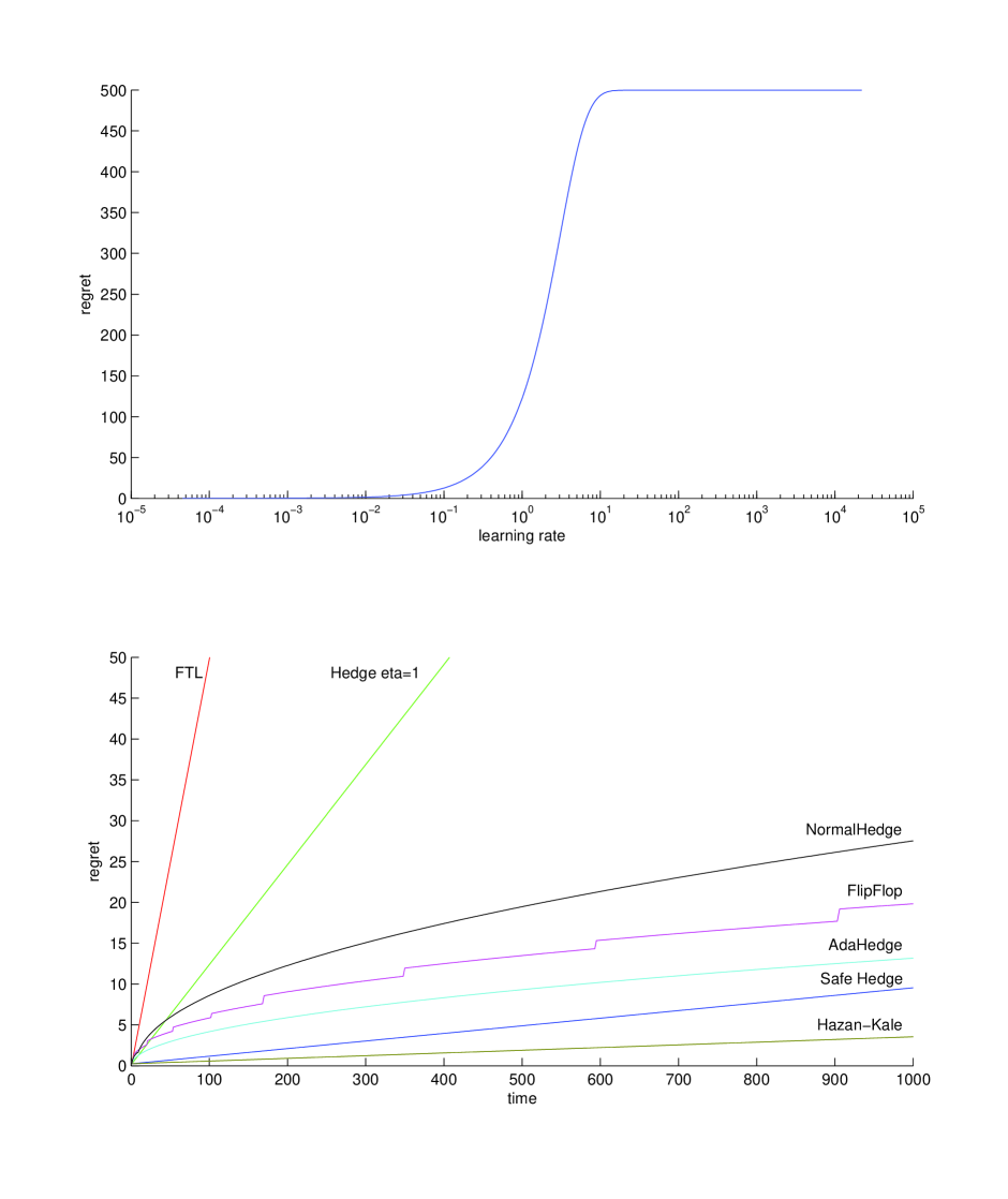
5.1 Experiment 1. Worst case for FTL
The experiment is defined by , and . This yields a loss matrix that starts as follows:
These data are the worst case for FTL: each round, the leader incurs loss one, while each of the two individual experts only receives a loss once every two rounds. Thus, the FTL regret increases by one every two rounds and ends up around 500. For any learning rate , the weights used by the Hedge algorithm are repeated every two rounds, so the regret increases by the same amount every two rounds: the regret increases linearly in for every fixed that does not vary with . However, the constant of proportionality can be reduced greatly by reducing the value of , as the top graph in Figure 3 shows: for , the regret becomes negligible for any less than about . Thus, in this experiment, a learning algorithm must reduce the learning rate to shield itself from incurring an excessive overhead.
The bottom graph in Figure 3 shows the expected breakdown of the FTL algorithm; Hedge with fixed learning rate also performs quite badly. When is reduced to the value that optimises the worst-case bound, the regret becomes competitive with that of the other algorithms. Note that Hazan and Kale’s algorithm has the best performance; this is because its learning rate is tuned in relation to the bound proved in the paper, which has a relatively large constant in front of the leading term. As a consequence the algorithm always uses a relatively small learning rate, which turns out to be helpful in this case but harmful in later experiments.
The FlipFlop algorithm behaves as theory suggests it should: its regret increases alternately like the regret of AdaHedge and the regret of FTL. The latter performs horribly, so during those intervals the regret increases quickly, on the other hand the FTL intervals are relatively short-lived so they do not harm the regret by more than a constant factor.
The NormalHedge algorithm still has acceptable performance, although it is relatively large in this experiment; we have no explanation for this but in fairness we do observe good performance of NormalHedge in the other three experiments as well as in numerous further unreported simulations.
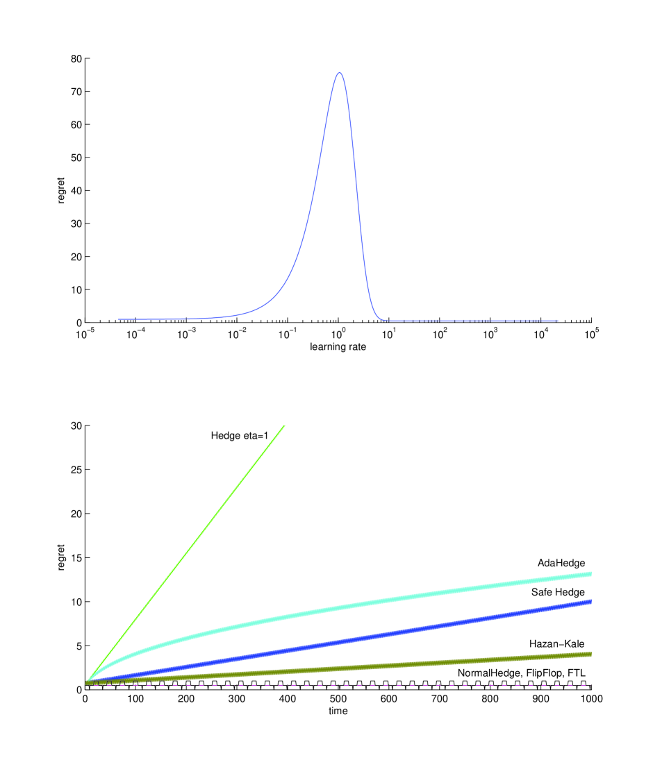
5.2 Experiment 2. Best case for FTL
The second experiment is defined by , and . The induced loss matrix starts as follows:
These data look very similar to the first experiment, but as the top graph in Figure 4 illustrates, because of this small change, it is now viable to reduce the regret by using a very large learning rate. In particular, since there are no leader changes after the first round, FTL incurs a regret of only .
As in the first experiment, the regret increases linearly in for every fixed (provided it is less than ); but now the constant of linearity is large only for learning rates close to . Once FlipFlop enters the FTL regime for the second time, it stays there indefinitely, which results in bounded regret. We observe that NormalHedge adapts in the same way to these data. The behaviour of the other algorithms is very similar to the first experiment, and as a consequence their regret grows without bound.
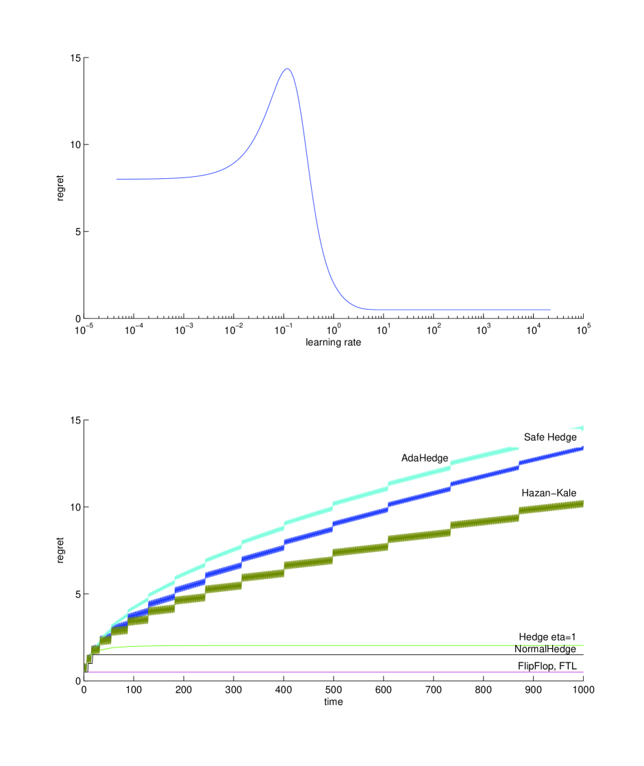
5.3 Experiment 3. Weights do not concentrate in AdaHedge
The third experiment uses , and . The first few loss vectors are the same as in the previous experiment, but every now and then there are two loss vectors in a row, so that the first expert gradually falls behind the second in terms of performance. By , the first expert has accumulated 508 loss, while the second expert has only 492.
For any fixed learning rate , the weights used by Hedge now concentrate on the second expert. We know from Lemma 4 that the mixability gap in any round is bounded by a constant times the variance of the loss under the weights played by the algorithm; as these weights concentrate on the second expert, this variance must go to zero. One can show that this happens quickly enough for the cumulative mixability gap to be bounded for any fixed that does not vary with or depend on . From (4) we have
So in this scenario, as long as the learning rate is kept fixed, we will eventually learn the identity of the best expert. However, if the learning rate is very small, this will happen so slowly that the weights still have not converged by . Even worse, the top graph in Figure 5 shows that for intermediate values of the learning rate, not only do the weights fail to converge on the second expert sufficiently quickly, but they are sensitive enough to increase the overhead incurred each round.
For this experiment, it really pays to use a large learning rate rather than a safe small one. Thus FTL, Hedge with , FlipFlop and NormalHedge perform excellently, while safe Hedge, AdaHedge and Hazan and Kale’s algorithm incur a substantial overhead. Extrapolating the trend in the graph, it appears that the overhead of these algorithms is not bounded. This is possible because the three algorithms with poor performance use a learning rate that decreases as a function of . As a concequence the used learning rate may remain too small for the weights to concentrate. For the case of AdaHedge, this is an example of the “nasty feedback loop” described in Section 3.
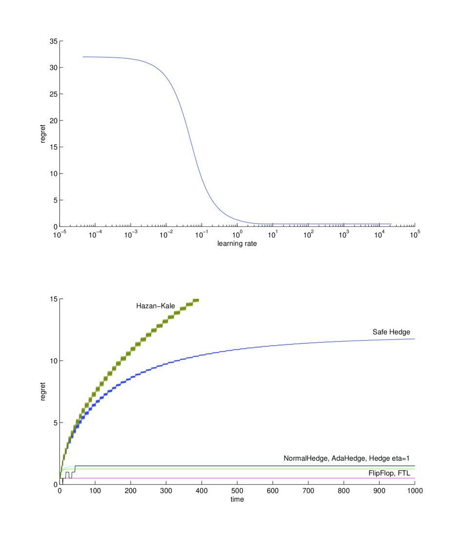
5.4 Experiment 4. Weights do concentrate in AdaHedge
The fourth and last experiment uses , and . The losses are comparable to those of the third experiment, but the performance gap between the two experts is somewhat larger. By , the two experts have loss 532 and 468, respectively. It is now so easy to determine which of the experts is better that the top graph in Figure 6 is nonincreasing: the larger the learning rate, the better.
The algorithms that managed to keep their regret bounded in the previous experiment obviously still perform very well, but it is clearly visible that AdaHedge now achieves the same. As discussed below Theorem 6, this happens because the weight concentrates on the second expert quickly enough that AdaHedge’s regret is bounded in this setting. Thus, while the previous experiment shows that AdaHedge can be tricked into reducing the learning rate while it would be better not to do so, the present experiment shows that on the other hand, sometimes AdaHedge does adapt really nicely to easy data, in contrast to algorithms that are tuned in terms of a worst-case bound.
6 Discussion and Conclusion
The main contributions of this work are twofold. First, we develop a new hedging algorithm called AdaHedge. The analysis simplifies existing results and we obtain improved bounds (Theorems 6 and 8). Moreover, AdaHedge is the first sophisticated Hedge algorithm that is “fundamental”, i.e. its weights are invariant under translation and scaling of the losses (Section 4). Second, we explain in detail why it is difficult to tune the learning rate such that good performance is obtained both for easy and for hard data, and we address the issue by developing the FlipFlop algorithm. FlipFlop never performs much worse than the Follow-the-Leader strategy, which works very well on easy data (Lemma 9), but it also retains a worst-case bound similar to the bound for AdaHedge (Theorem 14). As such, this work may be seen as solving a special case of a more general question. Below we briefly address this question and then place this work in a broader context, which provides an ambitious agenda for future work.
6.1 General Question: Competing with Hedge for any fixed learning rate
FlipFlop has regret to within a multiplicative constant of Hedge with learning rate (FTL) and Hedge with a variable, nonincreasing learning rate which achieves optimal regret in the worst-case. It is now natural to ask whether we can design a “Universal Hedge” algorithm that can compete with Hedge with any fixed learning rate . That is, for all , the regret up to time of Universal Hedge should be within a constant factor of the regret incurred by Hedge run with the fixed that minimizes the Hedge loss . This appears to be a difficult question, and maybe such an algorithm does not even exist. Yet even partial results (such as an algorithm that competes with or with a factor that increases slowly, say, logarithmically, in ) would already be of significant interest.
In this regard, it is interesting to note that in practical applications, the learning rates chosen by sophisticated versions of Hedge do not always perform very well; higher learning rates often do better. This is noted by Devaine et al. (2012), who resolve this issue by adapting the learning rate sequentially in an ad-hoc fashion which works well in their application, but for which they can provide no guarantees. A Universal Hedge algorithm would adapt to the optimal learning rate-with-hindsight. FlipFlop is a first step in this direction. Indeed, it already has some of the properties of such an ideal algorithm: under some conditions we can show that if Hedge achieves bounded regret using any learning rate, then FTL, and therefore FlipFlop, also achieves bounded regret:
Theorem 18
Fix any . For experts with losses in we have
The proof is in Appendix B. While the second implication remains valid for more experts and other losses, we currently do not know if the first implication continues to hold as well.
6.2 The Big Picture
Broadly speaking, a “learning rate” is any single scalar parameter controlling the relative weight of the data and a prior regularization term in a learning task. Such learning rates pop up in batch settings as diverse as -regularized regression such as Lasso and Ridge, standard Bayesian nonparametric and PAC-Bayesian inference (Zhang, 2006; Audibert, 2004; Catoni, 2007), and — as in this paper — in sequential prediction. In batch settings one may sometimes set the learning rate by cross-validation, but this does not always come with theoretical guarantees, and cannot easily be extended to the sequential prediction setting. In a Bayesian approach, one can set the learning rate by treating it as just another parameter, equipping it with a prior and marginalizing or determining the MAP value; it is known that this can fail dramatically however, if all the models under consideration are wrong (Grünwald, 2012). All the applications just mentioned are similar in that they can formally be seen as variants of Bayesian inference — Bayesian MAP in Lasso and Ridge, randomized drawing from the posterior (“Gibbs sampling”) in the PAC-Bayesian setting and Hedge in the setting of this paper. An ideal method for adapting the learning rate would work in all such cases. We currently have methods that are guaranteed to work for a few special cases (see Table 2). It is encouraging that all these methods are based on the same, apparently fundamental, quantity, the mixability gap as defined before Lemma 1: they all employ different techniques to ensure a learning rate under which the posterior is concentrated and hence the mixability gap is small. This gives some hope that the approach can be taken even further.
method mode complexity setting minimizes competes with best in: predicts/ estimates FlipFlop sequential finite worst-case regret averages prediction safe two-part MDL (Grünwald, 2011) batch countably infinite stochastic, i.i.d. excess risk point safe Bayes (Grünwald, 2012) batch completely arbitrary stochastic, i.i.d. excess risk averages
In Table 2, “complexity” refers to the maximum number of actions/experts in the DTOL setting of FlipFlop and the maximum number of predictors (e.g. classifiers, regression functions) with prior support in the stochastic setting. In the stochastic setting we invariably assume that data are of the form and the goal is to predict based on . is defined as the set . The Safe Bayes and MDL algorithms may even be capable of competing with the best . While we currently do not know whether this is the case, we note that, in the stochastic setting, being able to compete with the best is already satisfactory: it implies that one can achieve minimax optimal risk convergence rates in a variety of settings, e.g. if a Tsybakov margin condition holds (Grünwald, 2012).
The safe two-part MDL estimator produces point estimates of the best available predictors; analogously to FlipFlop, the safe Bayesian estimator averages all predictors according to its posterior. The two “safe” algorithms can deal with arbitrary loss functions as long as the loss is almost surely bounded. If the data are sampled from a distribution with bounded support, this even holds if the loss function is itself unbounded.
All this suggests a major goal for future work: extending the worst-case approach of this paper to the settings that are currently dealt with only in the stochastic case. First, as already explained above, we would like to be able to compete with all in some set that contains a whole range rather than just two values. Second, we would like to compete with the best in a setting with a countably infinite number of experts equipped with an arbitrary prior mass function . Third, as an ultimate goal, we would like to develop a method that can compete with the best with completely arbitrary sets of experts equipped with some prior distribution . The second and third goal require a slight modification of the type of results in this paper: currently, our results all start with the basic identity and bound (6), repeated here for convenience:
For the case of infinitely many experts, this should be replaced by the following identity and inequality, which hold simultaneously for all distributions on the set of experts; the idea is to choose so as to get a useful bound.
| (24) |
where for convenience we defined , the expected value of the cumulative loss under distribution . Here is a user-defined prior distribution on the set of experts, analogous to our probability mass function , and denotes the KL divergence between two distributions on experts. The inequality is trivial; the equality is a well-known result both in the sequential prediction and the PAC-Bayesian literature; see e.g. Zhang (2006). To make (6.2) more concrete, consider a countable set of experts, fix an expert and take to be a point mass on . Then and becomes equal to , so (6.2) can be further rewritten as
We hope that using this bound, analogously to our use of (6) in the current paper, one can prove bounds similar to those appearing in Theorem 8 and 14, with all occurrences of and replaced by and . Here can be thought of as a ‘comparator’ expert, and the bounds should hold uniformly for all but get progressively weaker for with small initial prior weight . For the case of uncountable sets of experts, the hope is again to prove results similar to Theorem 8 and 14, but now based on (6.2). Such results would give strong worst-case performance bounds on huge, “nonparametric” sets of experts such as Gaussian process models. Currently such worst-case bounds exist for the logarithmic loss (Kakade et al., 2006), but not for any other loss function.
Acknowledgments
We would like to thank Wojciech Kotłowski and Gilles Stoltz for critical feedback. This work was supported in part by the IST Programme of the European Community, under the PASCAL Network of Excellence, IST-2002-506778 and by NWO Rubicon grants 680-50-1010 and 680-50-1112.
A Proof of Lemma 1
The result for follows from as a limiting case, so we may assume without loss of generality that . Then is obtained by using Jensen’s inequality to move the logarithm inside the expectation, and and follow by bounding all losses by their minimal and maximal values, respectively. The next two items are analogues of similar basic results in Bayesian probability. Item 2 generalizes the chain rule of probability :
For the third item, use item 2 to write
The lower bound is obtained by bounding all from below by ; for the upper bound we drop all terms in the sum except for the term corresponding to the best expert and use .
For the last item, let be any two learning rates. Then Jensen’s inequality gives
This completes the proof.
B Proof of Theorem 18
Suppose that FTL has unbounded regret. We argue that Hedge with fixed must have unbounded regret as well. First remove all trials where both experts suffer the same loss, as these trials do not change the regret of either FTL or Hedge. Abbreviate . We say that a leader change happens at when , that is, crosses zero at . Since FTL has unbounded regret, there are infinitely many leader changes.
We call a point-pair a local extremum if the losses in trials and are opposite, i.e. . Observe that a leader change can not be a local extremum. Over a local extremum, Hedge suffers loss but the best expert only suffers loss . The regret of Hedge is hence decreased when the trials and are removed. Iterated removal of local extrema leads to the sequence
The regret of Hedge on this sequence is linear in . To see this, observe that over one period the loss of the best expert increases by , while the loss of Hedge increases by
Hence the Hedge regret is unbounded on the original loss sequence.
References
- Audibert (2004) Jean-Yves Audibert. PAC-Bayesian statistical learning theory. PhD thesis, Université Paris VI, 2004.
- Auer et al. (2002) Peter Auer, Nicolò Cesa-Bianchi, and Claudio Gentile. Adaptive and self-confident on-line learning algorithms. Journal of Computer and System Sciences, 64:48–75, 2002.
- Catoni (2007) Olivier Catoni. PAC-Bayesian Supervised Classification. Lecture Notes-Monograph Series. IMS, 2007.
- Cesa-Bianchi and Lugosi (2006) Nicolò Cesa-Bianchi and Gábor Lugosi. Prediction, learning, and games. Cambridge University Press, 2006.
- Cesa-Bianchi et al. (1997) Nicolò Cesa-Bianchi, Yoav Freund, David Haussler, David P. Helmbold, Robert E. Schapire, and Manfred K. Warmuth. How to use expert advice. Journal of the ACM, 44(3):427–485, 1997.
- Cesa-Bianchi et al. (2007) Nicolò Cesa-Bianchi, Yishay Mansour, and Gilles Stoltz. Improved second-order bounds for prediction with expert advice. Machine Learning, 66(2/3):321–352, 2007.
- Chaudhuri et al. (2009) Kamalika Chaudhuri, Yoav Freund, and Daniel Hsu. A parameter-free hedging algorithm. In Advances in Neural Information Processing Systems 22 (NIPS 2009), pages 297–305, 2009.
- Chernov and Vovk (2010) Alexey V. Chernov and Vladimir Vovk. Prediction with advice of unknown number of experts. In Peter Grünwald and Peter Spirtes, editors, UAI, pages 117–125. AUAI Press, 2010.
- Devaine et al. (2012) Marie Devaine, Pierre Gaillard, Yannig Goude, and Gilles Stoltz. Forecasting electricity consumption by aggregating specialized experts; a review of the sequential aggregation of specialized experts, with an application to Slovakian and French country-wide one-day-ahead (half-)hourly predictions. Machine Learning, 2012. To appear.
- Freund and Schapire (1997) Yoav Freund and Robert E. Schapire. A decision-theoretic generalization of on-line learning and an application to boosting. Journal of Computer and System Sciences, 55:119–139, 1997.
- Freund and Schapire (1999) Yoav Freund and Robert E. Schapire. Adaptive game playing using multiplicative weights. Games and Economic Behavior, 29:79–103, 1999.
- Gerchinovitz (2011) Sébastien Gerchinovitz. Prédiction de suites individuelles et cadre statistique classique: étude de quelques liens autour de la régression parcimonieuse et des techniques d’agrégation. PhD thesis, Université Paris-Sud, 2011.
- Grünwald (2011) Peter Grünwald. Safe learning: bridging the gap between Bayes, MDL and statistical learning theory via empirical convexity. In Proceedings of the 24th International Conference on Learning Theory (COLT 2011), pages 551–573, 2011.
- Grünwald (2012) Peter Grünwald. The safe Bayesian: learning the learning rate via the mixability gap. In Proceedings of the 23rd International Conference on Algorithmic Learning Theory (ALT 2012), 2012.
- Hazan and Kale (2008) Elad Hazan and Satyen Kale. Extracting certainty from uncertainty: Regret bounded by variation in costs. In Proceedings of the 21st Annual Conference on Learning Theory (COLT), pages 57–67, 2008.
- Hutter and Poland (2005) Marcus Hutter and Jan Poland. Adaptive online prediction by following the perturbed leader. Journal of Machine Learning Research, 6:639–660, 2005.
- Kakade et al. (2006) Sham Kakade, Matthias Seeger, and Dean Foster. Worst-case bounds for Gaussian process models. In Proceedings of the 2005 Neural Information Processing Systems Conference (NIPS 2005), 2006.
- Kalai and Vempala (2003) Adam Kalai and Santosh Vempala. Efficient algorithms for online decision. In Proceedings of the 16st Annual Conference on Learning Theory (COLT), pages 506–521, 2003.
- Kalnishkan and Vyugin (2005) Yuri Kalnishkan and Michael V. Vyugin. The weak aggregating algorithm and weak mixability. In Proceedings of the 18th Annual Conference on Learning Theory (COLT), pages 188–203, 2005.
- Littlestone and Warmuth (1994) Nick Littlestone and Manfred K. Warmuth. The weighted majority algorithm. Information and Computation, 108(2):212–261, 1994.
- van Erven et al. (2011) Tim van Erven, Peter Grünwald, Wouter M. Koolen, and Steven de Rooij. Adaptive hedge. In Advances in Neural Information Processing Systems 24 (NIPS 2011), pages 1656–1664, 2011.
- Vovk (1998) Vladimir Vovk. A game of prediction with expert advice. Journal of Computer and System Sciences, 56(2):153–173, 1998.
- Vovk (2001) Vladimir Vovk. Competitive on-line statistics. International Statistical Review, 69(2):213–248, 2001.
- Vovk et al. (2005) Vladimir Vovk, Akimichi Takemura, and Glenn Shafer. Defensive forecasting. In Proceedings of AISTATS 2005, 2005. Archive version available at http://www.vovk.net/df.
- Zhang (2006) Tong Zhang. Information theoretical upper and lower bounds for statistical estimation. IEEE Transactions on Information Theory, 52(4):1307–1321, 2006.