Phase Structure in a Dynamical Soft-Wall Holographic QCD Model

Abstract

We consider the Einstein-Maxwell-dilaton system with an arbitrary kinetic gauge function and a dilaton potential. A family of analytic solutions is obtained by the potential reconstruction method. We then study its holographic dual QCD model. The kinetic gauge function can be fixed by requesting the linear Regge spectrum of mesons. We calculate the free energy to obtain the phase diagram of the holographic QCD model and interpret our result as the heavy quarks system by comparing the recent lattice QCD simulation. We finally obtain the equations of state in our model.

I Introduction

To study phase structure of QCD is a challenging and important task. It is well known that QCD is in the confinement and chiral symmetry breaking phase for the low temperature and small chemical potential, while it is in the deconfinement and chiral symmetry restored phase for the high temperature and large chemical potential. Thus it is widely believed that there exists a phase transition between these two phases. To obtain the phase transition line in the $T-\mu$ phase diagram is a rather difficult task because the QCD coupling constant becomes very strong near the phase transition region and the conventional perturbative method does not work well. Moreover, with the nonzero physical quark masses presented, part of the phase transition line will weaken to a crossover for a range of temperature and chemical potential that makes the phase structure of QCD more complicated. Locating the critical point where the phase transition converts to a crossover is another challenging work. For a long time, lattice QCD is the only method to attack these problems. Although lattice QCD works well for zero density, it encounters the sign problem when considering finite density, i.e. $\mu\neq 0$. However, the most interesting region in the QCD phase diagram is at finite density. The most concerned subjects, such as heavy-ion collisions and compact stars in astrophysics, are all related to QCD at finite density. Recently, lattice QCD has developed some techniques to solve the sign problem, such as reweighting method, imaginary chemical potential method and the method of expansion in $\mu/T$. Nevertheless, these techniques are only able to deal with the cases of small chemical potentials and quickly lost control for the larger chemical potential. See 1009.4089 for a review of the current status of lattice QCD.

On the other hand, using the idea of AdS/CFT duality from string theory, one is able to study QCD in the strongly coupled region by studying its weakly coupled dual gravitational theory, i.e. holographic QCD. The models which are directly constructed from string theory are called the top-down models. The most popular top-down models are D3-D7 0306018 ; 0311270 ; 0304032 ; 0611099 model and D4-D8 (Sakai-Sugimoto) model 0412141 ; 0507073 . In these top-down holographic QCD models, confinement and chiral symmetry phase transitions in QCD have been addressed and been translated into geometric transformations in the dual gravity theory. Meson spectrums and decay constants have also been calculated and compared with the experimental data with surprisingly consistency. Although the top-down QCD models describe many important properties in realistic QCD, the meson spectrums obtained from those models can not realize the linear Regge trajectories. To solve this problem, another type of holographic models have been developed, i.e. bottom-up models, such as the hard wall model 0501128 and the later refined soft-wall model 0602229 . In the original soft-wall model, the IR correction of the dilaton field was put by hand to obtain the linear Regge behavior of the meson spectrum. However, since the fields configuration is put by hand, it does not satisfy the equations of motion. To get a fields configuration which is both consistent with the equation of motions and realizes the linear Regge trajectory, dynamical soft-wall models were constructed by introduce a dilaton potential 0801.4383 ; 0806.3830 consistently. Later on, the Einstein-dilaton and Einstein-Maxwell-dilaton models have been widely studied numerically 0804.0434 ; 1006.5461 ; 1012.1864 ; 1108.2029 ; 1201.0820 . By potential reconstruction method, analytic solutions can be obtained in the Einstein-dilaton model 1103.5389 and similarly in the Einstein-Maxwell-dilaton model 1201.0820 ; 1209.4512 .

In this paper, we consider the Einstein-Maxwell-dilaton system with an arbitrary kinetic gauge function and a dilaton potential. A family of analytic solutions are obtained by the potential reconstruction method. We then study its holographic dual QCD model. The kinetic gauge function can be fixed by requesting the meson spectrums satisfy the linear Regge trajectories. We study the thermodynamics of the Einstein-Maxwell-dilaton background and calculate the free energy to obtain the phase diagram of the holographic QCD model. By comparing our result with the recent lattice QCD simulations, we interpret our system as the model for the heavy quarks system. We finally compute the different equation of states in our model and discuss their behaviors. The behavior of the equations of state is consistent with our interpretation of the heavy quarks.

The paper is organized as follows. In section II, we consider the Einstein-Maxwell-dilaton system with a dilaton potential as well as a gauge kinetic function. By potential reconstruction method, we obtain a family of analytic solutions with arbitrary gauge kinetic function and warped factor. We then fix the gauge kinetic function by requesting the meson spectrums to realize the linear Regge trajectories. By choosing a proper warped factor, we obtain the final form of our analytic solution. In section III, we study the thermodynamics of our gravitational background and compute the free energy to get the phase diagram. From the phase diagram, we argue that our background is dual to QCD with heavy quarks and interpret the black hole phase transition as the deconfinement phase transition in QCD. We finally plot the equations of state in our background to compare with that in QCD. We conclude our result in section IV.

II Einstein-Maxwell-Dilaton System

We consider a 5-dimensional Einstein-Maxwell-dilaton system with probe matters. The action of the system have two parts, the background part and the matter part,

$$S=S_{b}+S_{m}.$$ (2.1)

In string frame, the background action includes a gravity field $g_{\mu\nu}^{s}$, a Maxwell field $A_{\mu}$ and a neutral dilatonic scalar field $\phi_{s}$,

$$S_{b}=\dfrac{1}{16\pi G_{5}}\int d^{5}x\sqrt{-g^{s}}e^{-2\phi_{s}}\left[{R}_{s}-{\frac{f_{s}\left(\phi_{s}\right)}{4}F^{2}}+4\partial_{\mu}\phi_{s}\partial^{\mu}\phi_{s}-V_{s}\left(\phi_{s}\right)\right],$$ (2.2)

where $f_{s}\left(\phi_{s}\right)$ is the gauge kinetic function associated to the Maxwell field $A_{\mu}$ and $V_{s}\left(\phi_{s}\right)$ is the potential of the dilaton field. One should note that the function $f_{s}\left(\phi_{s}\right)$ is a positive-definite function. The explicit forms of the gauge kinetic function $f_{s}\left(\phi_{s}\right)$ and the dilaton potential $V_{s}\left(\phi_{s}\right)$ are not given ad hoc and will be solved consistently with the background.

The matter action includes the flavor fields $\left({A}_{\mu}^{L},{A}_{\mu}^{R}\right)$, which we will treat as probe, describing the degree of freedom of mesons on the 4d boundary,

$$S_{m}=-\dfrac{1}{16\pi G_{5}}\int d^{5}x\sqrt{-g^{s}}e^{-2\phi_{s}}{\frac{f_{s}\left(\phi_{s}\right)}{4}}\left({F_{L}^{2}+F_{R}^{2}}\right),$$ (2.3)

where ${G}_{5}$ is the coupling constant for the flavor field strength ${F}_{\mu\nu}{=\partial}_{\mu}A_{\nu}-{\partial}_{\nu}A_{\mu}$ and $f_{s}\left(\phi_{s}\right)$ is the gauge kinetic function associated to the flavor field. The gauge kinetic function of the flavor field in the matter action is not necessary to be the same as that of the Maxwell field in the background action [2.2] in general, but here we set them equal for simplicity.

In the above, we have defined our model in string frame in which it is natural to write the boundary conditions as we will see when solving the background in the next section. However, to study the thermodynamics of QCD at finite temperature, it is convenient to solve the equations of motion and study the equations of state in Einstein frame. To transform the action from string frame to Einstein frame, we make the following ”standard” transformations,

$$\phi_{s}=\sqrt{\dfrac{3}{8}}\phi\text{, \ \ }g_{\mu\nu}^{s}=g_{\mu\nu}{e}^{\sqrt{\tfrac{2}{3}}\phi}\text{, \ \ }f_{s}\left(\phi_{s}\right)=f\left(\phi\right){e}^{\sqrt{\tfrac{2}{3}}\phi}\text{, \ \ }V_{s}\left(\phi_{s}\right)={e}^{-\sqrt{\tfrac{2}{3}}\phi}V\left(\phi\right).$$ (2.4)

The background and the matter actions become, in Einstein frame,

$$S_{b} =\dfrac{1}{16\pi G_{5}}\int d^{5}x\sqrt{-g}\left[{R-\frac{f\left(\phi\right)}{4}F^{2}}-\dfrac{1}{2}\partial_{\mu}\phi\partial^{\mu}\phi-V\left(\phi\right)\right],$$ (2.5)

$$S_{m} =-\dfrac{1}{16\pi G_{5}}\int d^{5}x\sqrt{-g}{\frac{f\left(\phi\right)}{4}}\left({F_{V}^{2}+F_{\tilde{V}}^{2}}\right).$$ (2.6)

where we have written the flavor fields ${A}^{L}$ and ${A}^{R}$ in terms of the vector meson and pseudovector meson fields $V$ and $\tilde{V}$,

$${A}^{L}=V+\tilde{V}\text{, \ \ }{A}^{R}=V-\tilde{V}.$$ (2.7)

The equations of motion can be derived from the actions (2.5) and (2.6) as

$$\nabla^{2}\phi =\frac{\partial V}{\partial\phi}+\frac{1}{4}\frac{\partial f}{\partial\phi}\left(F^{2}+{F_{V}^{2}+F_{\tilde{V}}^{2}}\right),$$ (2.8)

$$\nabla_{\mu}\left[f(\phi)F^{\mu\nu}\right] ={{0,}}$$ (2.9)

$$\nabla_{\mu}\left[f(\phi)F_{V}^{\mu\nu}\right] ={{0,}}$$ (2.10)

$$\nabla_{\mu}\left[f(\phi)F_{\tilde{V}}^{\mu\nu}\right] ={0,}$$ (2.11)

$$R_{\mu\nu}-\frac{1}{2}g_{\mu\nu}R =\frac{f(\phi)}{2}\left(F_{\mu\rho}F_{\nu}^{\rho}-\frac{1}{4}g_{\mu\nu}F^{2}+\left\{{F_{V},F_{\tilde{V}}}\right\}\right)+\frac{1}{2}\left[\partial_{\mu}\phi\partial_{\nu}\phi-\frac{1}{2}g_{\mu\nu}\left(\partial\phi\right)^{2}-g_{\mu\nu}V\right].$$ (2.12)

In the next section, we will solve the above equations of motion under some physical boundary conditions and constraints.

II.1 The gravitational Background

In this section, we will solve the background of the Einstein-Maxwell-dilaton system defined in the last section. We first turn off the probe flavor field $V$ and $\tilde{V}$ in the equations of motion (2.8-2.12), which reduce to

$$\nabla^{2}\phi =\frac{\partial V}{\partial\phi}+\frac{F^{2}}{4}\frac{\partial f}{\partial\phi},$$ (2.13)

$$\nabla_{\mu}\left[f(\phi)F^{\mu\nu}\right] ={{0,}}$$ (2.14)

$$R_{\mu\nu}-\frac{1}{2}g_{\mu\nu}R =\frac{f(\phi)}{2}\left(F_{\mu\rho}F_{\nu}^{\rho}-\frac{1}{4}g_{\mu\nu}F^{2}\right)+\frac{1}{2}\left[\partial_{\mu}\phi\partial_{\nu}\phi-\frac{1}{2}g_{\mu\nu}\left(\partial\phi\right)^{2}-g_{\mu\nu}V\right].$$ (2.15)

Because we are interested in the black hole solutions, we consider the following form of the metric in Einstein frame,

$$ds^{2} =\dfrac{L^{2}e^{2A\left(z\right)}}{z^{2}}\left[-g(z)dt^{2}+\frac{dz^{2}}{g(z)}+d\vec{x}^{2}\right],$$ (2.16)

$$\phi =\phi\left(z\right)\text{, \ \ }A_{\mu}=A_{t}\left(z\right),$$ (2.17)

where $z=0$ corresponds to the conformal boundary of the 5d spacetime. We will set the radial $L$ of $AdS_{5}$ space to be unit in the following of this paper.

Using the ansatz of the metric, the Maxwell field and the dilaton field (2.16, 2.17), the equations of motion and constraints for the background fields become

$$\phi^{\prime\prime}+\left(\frac{g^{\prime}}{g}+3A^{\prime}-\dfrac{3}{z}\right)\phi^{\prime}+\left(\frac{z^{2}e^{-2A}A_{t}^{\prime 2}f_{\phi}}{2g}-\frac{e^{2A}V_{\phi}}{z^{2}g}\right) =0,$$ (2.18)

$$A_{t}^{\prime\prime}+\left(\frac{f^{\prime}}{f}+A^{\prime}-\dfrac{1}{z}\right)A_{t}^{\prime} =0,$$ (2.19)

$$A^{\prime\prime}-A^{\prime 2}+\dfrac{2}{z}A^{\prime}+\dfrac{\phi^{\prime 2}}{6} =0,$$ (2.20)

$$g^{\prime\prime}+\left(3A^{\prime}-\dfrac{3}{z}\right)g^{\prime}-e^{-2A}z^{2}fA_{t}^{\prime 2} =0,$$ (2.21)

$$A^{\prime\prime}+3A^{\prime 2}+\left(\dfrac{3g^{\prime}}{2g}-\dfrac{6}{z}\right)A^{\prime}-\dfrac{1}{z}\left(\dfrac{3g^{\prime}}{2g}-\dfrac{4}{z}\right)+\dfrac{g^{\prime\prime}}{6g}+\frac{e^{2A}V}{3z^{2}g} =0.$$ (2.22)

We should notice that only four of the above five equations are independent. In the following, we will solve the equations (2.19-2.22), and leave the equation (2.18) as a constraint for a consistent check.

To solve the background, we need to specify the boundary conditions. Near the horizon $z=z_{H}$, we require

$$A_{t}\left(z_{H}\right)=g\left(z_{H}\right)=0,$$ (2.23)

due to the physical requirement that $A_{\mu}A^{\mu}=g^{tt}A_{0}A_{0}$ must be finite at $z=z_{H}$.

Near the boundary $z\rightarrow 0$, we require the metric in string frame to be asymptotic to $AdS_{5}$, thus

$$ds_{z\rightarrow 0}^{2}=g_{\mu\nu}^{s}\left(z\rightarrow 0\right)dx^{\mu}dx^{\nu}=\dfrac{1}{z^{2}}\left[-dt^{2}+dz^{2}+d\vec{x}^{2}\right].$$ (2.24)

This boundary condition, in Einstein frame, becomes,

$$A\left(0\right)=-\sqrt{\dfrac{1}{6}}\phi\left(0\right)\text{, \ \ }g\left(0\right)=1.$$ (2.25)

Since we do not assume the form of the dilaton potential $V\left(\phi\right)$, which should be solved consistently from the equations of motion, we will treat the dilaton potential as a function of $z$, i.e. $V\left(z\right)$, when we solve the equations of motion. With the above boundary conditions (2.23) and (2.25), the equations of motion (2.19-2.22) can be analytically solved as

$$\phi^{\prime}\left(z\right) =\sqrt{-6\left(A^{\prime\prime}-A^{\prime 2}+\dfrac{2}{z}A^{\prime}\right)},$$ (2.26)

$$A_{t}\left(z\right) =\sqrt{\dfrac{-1}{\int_{0}^{z_{H}}y^{3}e^{-3A}dy\int_{y_{g}}^{y}\dfrac{x}{e^{A}f}dx}}\int_{z_{H}}^{z}\dfrac{y}{e^{A}f}dy,$$ (2.27)

$$g\left(z\right) =1-\dfrac{\int_{0}^{z}y^{3}e^{-3A}dy\int_{y_{g}}^{y}\dfrac{x}{e^{A}f}dx}{\int_{0}^{z_{H}}y^{3}e^{-3A}dy\int_{y_{g}}^{y}\dfrac{x}{e^{A}f}dx},$$ (2.28)

$$V\left(z\right) =-3z^{2}ge^{-2A}\left[A^{\prime\prime}+3A^{\prime 2}+\left(\dfrac{3g^{\prime}}{2g}-\dfrac{6}{z}\right)A^{\prime}-\dfrac{1}{z}\left(\dfrac{3g^{\prime}}{2g}-\dfrac{4}{z}\right)+\dfrac{g^{\prime\prime}}{6g}\right],$$ (2.29)

where we have used the boundary conditions to fix most of the integration constants. The only undetermined integration constant $y_{g}$ will be related to the chemical potential $\mu$ in the following way. We expand the field $A_{t}\left(z\right)$ near the boundary at $z=0$ to get

$$A_{t}\left(0\right)=\sqrt{\dfrac{-1}{\int_{0}^{z_{H}}y^{3}e^{-3A}dy\int_{y_{g}}^{y}\dfrac{x}{e^{A}f}dx}}\left(-\int_{0}^{z_{H}}\dfrac{y}{e^{A}f}dy+\dfrac{1}{e^{A\left(0\right)}f\left(0\right)}z^{2}+\cdots\right).$$ (2.30)

Using the AdS/CFT dictionary, we can define the chemical potential in our system as

$$\mu=-\sqrt{\dfrac{-1}{\int_{0}^{z_{H}}y^{3}e^{-3A}dy\int_{y_{g}}^{y}\dfrac{x}{e^{A}f}dx}}\int_{0}^{z_{H}}\dfrac{y}{e^{A}f}dy,$$ (2.31)

in which $y_{g}$ can be solved in term of the chemical potential $\mu$ once the gauge kinetic function $f\left(z\right)$ and the warped factor $A\left(z\right)$ are given. Put the solution (2.26-2.29) into the constraint (2.18), it is straightforward to verify that the above solutions are consistent with the constraint.

We note that the solutions (2.26-2.29) depend on two arbitrary functions, i.e. the gauge kinetic function $f\left(z\right)$ and the warped factor $A\left(z\right)$. Different choices of the functions $f\left(z\right)$ and $A\left(z\right)$ will give different physically allowed backgrounds. Thus we have just found a family of analytic solutions for the Einstein-Maxwell-dilaton system. We will use the freedom of choosing functions $f\left(z\right)$ and $A\left(z\right)$ to satisfy some extra important physical constraints.

II.2 Vector Meson Spectrum

In a theory with linear confinement like QCD, the spectrum of the squared mass $m_{n}^{2}$ of mesons is expected to grow as $n$ at zero temperature and zero density. This is known as the linear Regge trajectories 0507246 . In the method of AdS/QCD duality, this issue was first addressed in 0602229 by modifying the dilaton field in the IR region with a $z^{2}$ term, i.e. the soft-wall model. In 0602229 , the $z^{2}$ term was added by hand to the dilaton field. It means that the fields configuration used in the soft-wall model is not a solution of the Einstein equations. Dynamically generating the $z^{2}$ term by consistently solving the Einstein equations has been considered in several later works 1103.5389 ; 1104.4182 by including a proper dilaton potential. At finite temperature and density, the temperature dependent meson spectrum has been studied in 0703172 ; 0903.2316 ; 0911.2298 ; 1107.2738 ; 1112.5923 ; 1209.4198 with the AdS thermal gas background replaced by the charged AdS black hole background.

In the previous section, we consistently solved the equations of motion (2.18-2.22) for the Einstein-Maxwell-dilaton system. The analytic solutions depend on two arbitrary functions, the gauge kinetic function $f\left(z\right)$ and the warped factor $A\left(z\right)$. In this section, we will study the meson spectrum in our background and constrain the functions of $f\left(z\right)$ and $A\left(z\right)$ by requesting the vector meson spectrums satisfy the linear Regge trajectories at zero temperature and zero density.

We consider a 5d probe vector field $V$ whose action has been written down in (2.6),

$$S_{m}=-\dfrac{1}{16\pi G_{5}}\int d^{5}x\sqrt{-g}{\frac{f\left(\phi\right)}{4}F_{V}^{2}}.$$ (2.32)

To get the meson spectrum, we study the vector field $V$ in the charged AdS black hole background which we have obtained in the previous section,

$$ds^{2} =\dfrac{e^{2A\left(z\right)}}{z^{2}}\left[-g(z)dt^{2}+\frac{dz^{2}}{g(z)}+d\vec{x}^{2}\right]$$ (2.33)

$$A_{\mu} =A_{t}\left(z\right)dt.$$ (2.34)

The equation of motion of the vector field $V$ has been derived in (2.10) as

$$\nabla_{\mu}\left[f\left(\phi\right)F_{V}^{\mu\nu}\right]={{0.}}$$ (2.35)

Following 0602229 , we first use the gauge invariance to fix the gauge $V_{z}=0$, then the equation of motion of the transverse vector field $V_{\mu}$ $\left(\partial^{\mu}V_{\mu}=0\right)$ in the background (2.33) reduces to

$$\dfrac{1}{g}\nabla^{2}V_{i}+V_{i}^{\prime\prime}+\left(\dfrac{g^{\prime}}{g}+\dfrac{f^{\prime}}{f}+A^{\prime}-\dfrac{1}{z}\right)V_{i}^{\prime}=0,$$ (2.36)

where the prime is the derivative of $z$. We next perform the Fourier transformation for the vector field $V_{i}$ as

$$V_{i}\left(x,z\right)=\int\dfrac{d^{4}k}{\left(2\pi\right)^{4}}e^{ik\cdot x}v_{i}\left(z\right),$$ (2.37)

where $k=\left(\omega,\vec{p}\right)$ and the functions $v_{i}\left(z\right)$ satisfy the eigen-equations

$$-v^{\prime\prime}_{i}-\left(\dfrac{g^{\prime}}{g}+\dfrac{f^{\prime}}{f^{\prime}}+A^{\prime}-\dfrac{1}{z}\right)v^{\prime}_{i}=\left(\dfrac{\omega^{2}}{g^{2}}-\dfrac{p^{2}}{g}\right)v_{i}.$$ (2.38)

Redefining the functions $v_{i}\left(z\right)$ with

$$v_{i}=\left(\dfrac{z}{e^{A}fg}\right)^{1/2}\psi_{i}\equiv X\psi_{i},$$ (2.39)

brings the equation of motion (2.38) into the form of the Schrödinger equation

$$-\psi^{\prime\prime}_{i}+U\left(z\right)\psi_{i}=\left(\dfrac{\omega^{2}}{g^{2}}-\dfrac{p^{2}}{g}\right)\psi_{i},$$ (2.40)

where the potential function is

$$U\left(z\right)=\dfrac{2X^{\prime 2}}{X^{2}}-\dfrac{X^{\prime\prime}}{X}.$$ (2.41)

In the case of zero temperature and zero chemical potential, we expect that the discrete spectrum of the vector mesons obeys the linear Regge trajectories. At $\mu=0$, the metric of the zero temperature background (thermal gas) coincides with the black hole metric in the limit of zero size, i.e. $z_{H}\rightarrow\infty$, which corresponds to $g\left(z\right)=1$. In the zero size black hole limit, the Schrödinger equation reduces to

$$-\psi^{\prime\prime}_{i}+U\left(z\right)\psi_{i}=m^{2}\psi_{i},$$ (2.42)

where $-m^{2}=k^{2}=-\omega^{2}+p^{2}$. To produce the discrete mass spectrum with the linear Regge trajectories, the potential $U\left(z\right)$ should be in certain forms. Following 0602229 , a simple choice is to fix the gauge kinetic function as $f\left(z\right)=e^{\pm cz^{2}-A\left(z\right)}$, then the potential becomes

$$U\left(z\right)=-\dfrac{3}{4z^{2}}-c^{2}z^{2}.$$ (2.43)

The Schrödinger equations (2.40) with the above potential (2.43) have the discrete eigenvalues

$$m_{n}^{2}=4cn,$$ (2.44)

which is linear in the energy level $n$ as we expect for the vector spectrum at zero temperature and zero density. At finite temperature and finite density, $g\left(z\right)\neq 1$, the masses of the vector mesons solved from the Eq. (2.40) will depend on the temperature and density. For the case of small enough temperature and density, Eq. (2.40) can be solved perturbatively to get the mass shift from the linear Regge trajectories 1209.4198 ; 1112.5923 ; 1107.2738 ; 0801.4383 . For large temperature and density, the method of spectral functions is useful. The study of temperature and density dependent vector mass spectrum is in progress.

Once we fixed the gauge kinetic function $f=e^{\pm cz^{2}-A\left(z\right)}$, the Eq.(2.31) can be solved to get the integration constant $y_{g}$ in term of the chemical potential $\mu$ explicitly as

$$e^{cy_{g}^{2}}=\dfrac{\int_{0}^{z_{H}}y^{3}e^{-3A}e^{cy^{2}}dy}{\int_{0}^{z_{H}}y^{3}e^{-3A}dy}+\dfrac{\left(1-e^{cz_{H}^{2}}\right)^{2}}{2c\mu^{2}\int_{0}^{z_{H}}y^{3}e^{-3A}dy}.$$ (2.45)

Put the integration constant $y_{g}$ back into the solution (2.26-2.29), we can finally write down our solution as

$$\phi^{\prime}\left(z\right) =\sqrt{-6\left(A^{\prime\prime}-A^{\prime 2}+\dfrac{2}{z}A^{\prime}\right)},$$ (2.46)

$$A_{t}\left(z\right) =\mu\dfrac{e^{cz^{2}}-e^{cz_{H}^{2}}}{1-e^{cz_{H}^{2}}},$$ (2.47)

$$g\left(z\right) =1+\dfrac{1}{\int_{0}^{z_{H}}y^{3}e^{-3A}dy}\left[\dfrac{2c\mu^{2}}{\left(1-e^{cz_{H}^{2}}\right)^{2}}\left|\begin{array}[c]{cc}\int_{0}^{z_{H}}y^{3}e^{-3A}dy&\int_{0}^{z_{H}}y^{3}e^{-3A}e^{cy^{2}}dy\\ \int_{z_{H}}^{z}y^{3}e^{-3A}dy&\int_{z_{H}}^{z}y^{3}e^{-3A}e^{cy^{2}}dy\end{array}\right|-\int_{0}^{z}y^{3}e^{-3A}dy\right],$$ (2.50)

$$V\left(z\right) =-3z^{2}ge^{-2A}\left[A^{\prime\prime}+3A^{\prime 2}+\left(\dfrac{3g^{\prime}}{2g}-\dfrac{6}{z}\right)A^{\prime}-\dfrac{1}{z}\left(\dfrac{3g^{\prime}}{2g}-\dfrac{4}{z}\right)+\dfrac{g^{\prime\prime}}{6g}\right].$$ (2.51)

Now we have fixed all the integration constants by either satisfying the boundary conditions (2.23) and (2.25) or relating to the chemical potential $\mu$. The final solution (2.46-2.51) depends only on the warped factor $A\left(z\right)$. The choice of $A\left(z\right)$ is arbitrary provided it satisfies the boundary condition (2.25). In the next sections, we will make a simple choice of $A\left(z\right)$ and use it to study the phase structure in its holographic QCD model.

III Phase Structure

We will study the phase structure for the black hole background which we obtained in the last section (2.46-2.51). The phase transitions in the black hole background correspond to the phase transitions in its holographic QCD theory by AdS/QCD duality.

III.1 Fixing the Warped Factor

To be concrete, we fix the warped factor $A\left(z\right)$ in our solution in a simple form as

$$A\left(z\right)=-\dfrac{c}{3}z^{2}-bz^{4},$$ (3.1)

where the parameters $b$ and $c$ will be determined by later. It is easy to show that this choice of $A\left(z\right)$ satisfies the boundary condition (2.25) by Eq. (2.46). There are many more complicated choices for the function of $A\left(z\right)$, but we will show that our simple choice already educes abundant phenomena in QCD.

Once we choose the function of $A\left(z\right)$ up to the parameters $b$ and $c$, our solution (2.46-2.51) is completely fixed. Expanding the dilaton field and the dilaton potential near the boundary $z=0$, respectively,

$$\phi\left(z\right) =2\sqrt{3c}z+\dfrac{2\left(c^{2}+30b\right)}{9\sqrt{3c}}z^{3}+\cdots,$$ (3.2)

$$V =-12-18cz^{2}+\cdots,$$ (3.3)

we can write the dilaton potential in terms of the dilaton field $\phi$ as the expected form from the AdS/CFT dictionary,

$$V=-12+\dfrac{\Delta\left(\Delta-4\right)}{2}\phi^{2}+\cdots,\Delta=3.$$ (3.4)

The conformal dimension $\Delta=3$ satisfies the BF bound $2<\Delta<4$ implying that our gravitational background is stable. Furthermore, the dilaton satisfying the BF bound corresponds to a local, gauge invariant operator in 4d QCD possibly. One should note that the dilaton in our work is different from that in the references 1201.0820 ; 1103.5389 ; 1209.4512 , where the dictionary between the dilaton and gauge invariant operator in field theory are not clear. In our case, we combine the effects of quarks and gluon which absorbed by dilaton potential.

We fix the parameter $c$ by fitting our mass formula $m_{n}^{2}=4c\left(n+1\right)$ to the lowest two quarkonium states,

$$m_{J/\psi}=3.096GeV\text{,\ \ }m_{\psi^{\prime}}=3.685GeV,$$ (3.5)

For $c\simeq 1.16GeV^{2}$, we have

$$m_{1}=3.046GeV\text{,\ \ }m_{2}=3.731GeV,$$ (3.6)

which are consistent with the experimental data within $1\%$. The parameter $b$ will be determined later by comparing the the lattice QCD result of the phase transition temperature at zero chemical potential.

III.2 Black Hole Thermodynamics

Using the black hole metric we obtained

$$ds^{2}=\dfrac{e^{2A\left(z\right)}}{z^{2}}\left[-g(z)dt^{2}+\frac{dz^{2}}{g(z)}+d\vec{x}^{2}\right],$$ (3.7)

it is easy to calculate the Hawking-Bekenstein entropy

$$s=\dfrac{area\left(z_{H}\right)}{4}=\dfrac{e^{3A\left(z_{H}\right)}}{4z_{H}^{3}},$$ (3.8)

and the Hawking temperature

$$T=\dfrac{\kappa}{2\pi}=\dfrac{z_{H}^{3}e^{-3A\left(z_{H}\right)}}{4\pi\int_{0}^{z_{H}}y^{3}e^{-3A}dy}\left[1-\dfrac{2c\mu^{2}\left(e^{cz_{H}^{2}}\int_{0}^{z_{H}}y^{3}e^{-3A}dy-\int_{0}^{z_{H}}y^{3}e^{-3A}e^{cy^{2}}dy\right)}{\left(1-e^{cz_{H}^{2}}\right)^{2}}\right].$$ (3.9)

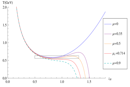
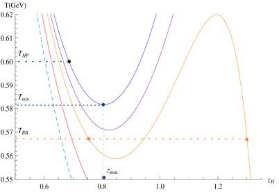
( a )                                                                 ( b )

Figure 1: The temperature v.s. horizon at the different chemical potentials $\mu=0,0.35,0.5,0.714,0.9GeV$ are plotted. We enlarge the rectangle region in (a) into (b) to see the detailed structure. At $\mu=0$, there is a global minimum $T_{\min}$; for $0<\mu<\mu_{c}\simeq 0.714GeV$, the minimum becomes local and eventually disappears for $\mu\geq\mu_{c}$.

We plot the temperature $T$ v.s. horizon $z_{H}$ at different chemical potentials in FIG. 1. At $\mu=0$, the temperature has a global minimum $T_{\min}$ at $z_{H}=z_{\min}$. For $z_{H}>z_{\min}$, the black hole solutions are thermodynamically unstable. Below the temperature $T_{\min}$, there is no black hole solution and we expect a Hawking-Page phase transition happens at a temperature $T_{HP}\gtrsim T_{\min}$ where the black hole background transits to a thermal gas background. For $0<\mu<\mu_{c}\simeq 0.714GeV$, the temperature has a local minimum/maximum temperature $T_{\mu\min}/T_{\mu\max}$ at $r_{H}=r_{\min}/r_{\max}$ and decreases to zero at a finite size of horizon. The black holes between $r_{\min}$ and $r_{\max}$ are thermodynamically unstable. We expect a similar Hawking-Page phase transition happens at a temperature $T_{HP}\gtrsim T_{\mu\min}$. In addition, since the thermodynamically stable black hole solutions exist even when the temperature below $T_{\mu\min}$, we also expect a black hole to black hole phase transition happens at a temperature $T_{BB}\in\left[T_{\mu\min},T_{\mu\max}\right]$, where the large black hole transits to a small black hole. The values of $T_{HP}$ and $T_{BB}$ will determine the true vacuum state, thermal gas or small black hole, in which the system will stay eventually. Finally, for $\mu>\mu_{c}$, the temperature monotonously decreases to zero and there is no black hole to black hole phase transition anymore, which implies that there is a second order phase transition happens at $\mu=\mu_{c}$, i.e. the critical point.

To determine the phase transition temperatures $T_{HP}$ and $T_{BB}$, we compute the free energy from the first law of thermodynamics in grand canonical ensemble,

$$F=\epsilon-Ts-\mu\rho.$$ (3.10)

Changes in the free energy of a system with constant volume are given by

$$dF=-sdT-\rho d\mu.$$ (3.11)

At fixed values of the chemical potential $\mu$, the free energy can be evaluated by the integral 0812.0792

$$F=-\int sdT.$$ (3.12)

We can fix the integration constant in the above integral (3.12) by considering the zero chemical potential case. At $\mu=0$, the metric of the zero temperature background (thermal gas) coincides with the black hole metric in the limit of zero size, i.e. $z_{H}\rightarrow\infty$, where we expect that the free energy of the black hole background also coincides with the free energy of the thermal gas background which we can choose to be zero. Thus we require $F\left(z_{H}\rightarrow\infty\right)=0$ and obtain that

$$F=\int_{z_{H}}^{\infty}s\dfrac{dT}{dz_{H}}dz_{H}.$$ (3.13)

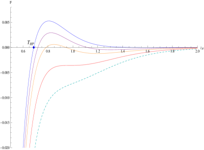
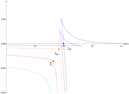
( a )                                                         ( b )

Figure 2: (a) The free energy v.s. horizon at the different chemical potentials $\mu=0,0.35,0.5,0.71,0.9$. At $\mu=0$, we normalized that the free energy vanishes when $z_{H}\rightarrow\infty$. For $\mu<\mu_{c}\simeq 0.71$, the free energy has a maximum; for $\mu\geq\mu_{c}$, the free energy becomes monotonous. (b) The free energy v.s. temperature at the different chemical potentials. At $\mu=0$, we normalized that the free energy vanishes when $z_{H}\rightarrow\infty$. For $\mu<\mu_{c}$, the free energy has a maximum; for $\mu\geq\mu_{c}$, the free energy becomes monotonous.

With the choice of $A\left(z\right)$ in (3.1), the integral in (3.13) can be performed to get the free energy of the black hole at fixed chemical potentials. We plot the free energy v.s. horizon at different chemical potentials in FIG. 2. We have normalized the free energy of the black holes by requiring it to vanish (or equal to the free energy of the thermal gas) at $z_{H}\rightarrow\infty$. Therefore, the black hole background is favored for the negative value of the free energy and the thermal gas background is favored for the positive value of the free energy. At $\mu=0$, the free energy starts from a large negative value at small $z_{H}$ to a positive maximum value and then decreases to zero at $z_{H}\rightarrow\infty$. The free energy intersecting the $x$-axis implies that there exists a Hawking-Page phase transition from the black hole to the thermal gas background at $T_{HP}$. For $0<\mu<\mu_{c}$, besides a maximum value, the free energy has a local minimum value, which implies a black hole to black hole phase transition. For $\mu\geq\mu_{c}$, the free energy becomes monotonous and no phase transition exists.

The phase structure is more transparent in the plot of free energy v.s. temperature in FIG. 2. At $\mu=0$, the free energy increase from a negative value with a large temperature to zero at $T=T_{HP}$ where the black hole transits to the thermal gas background which is thermodynamically stable for $T<T_{HP}$. At finite $\mu$, the free energy behaves as the expected swallow-tailed shape. For $0<\mu<\mu_{c}$, the curve of free energy intersects with itself at $T=T_{BB}$ where the large black hole transits to the small black hole background. We found that the free energy of the black hole is always less than that of the thermal gas, i.e. $F_{\text{black hole}}<F_{\text{thermal gas}}=0$. Therefore the thermodynamic system will always favor the small black hole background other than the thermal gas background when $T<T_{BB}$. When we increase the chemical potential $\mu$ from zero to $\mu_{c}$, the loop of the swallow-tailed shape shrinks to disappear at $\mu=\mu_{c}$, where the background undergoes a second phase transition. For $\mu>\mu_{c}$, the curve of the free energy increases smoothly from higher temperature to lower temperature.

Figure 3: The phase diagram in $T$ and $\mu$ plane. At small $\mu$, the system undergoes a first order phase transition at finite $T$. The first order phase transition stops at the critical point $\left(\mu_{c},T_{c}\right)\simeq\left(0.714GeV,0.528GeV\right)$, where the phase transition becomes second order. For $\mu>\mu_{c}$, the system weaken to a sharp but smooth crossover.

We plot the phase diagram of our holographic QCD model in FIG. 3. At $\mu=0$, the system undergoes a black hole to thermal gas first order phase transition at $T=T_{HP}$. For $0<\mu<\mu_{c}$, the system undergoes a large black hole to small black hole first order phase transition at $T_{BB}$. The phase transition temperature $T_{BB}$ approaches to $T_{HP}$ at $\mu\rightarrow 0$ that makes the phase diagram continuous at $\mu=0$. By comparing the phase transition temperature at $\mu=0$ to the lattice QCD simulation of $T_{HP}\simeq 0.6GeV$ in 1111.4953 , we fix the parameter $b\simeq 0.273GeV^{4}$. The first order phase transition stops at the critical point $\left(\mu_{c},T_{c}\right)$, where the phase transition becomes second order. For $\mu>\mu_{c}$, the system has a sharp but smooth crossover.

The phase diagram of our holographic QCD model in FIG. 3 is not expected from the common picture of QCD phase diagram, in which the transition is crossover for the small chemical potential $\mu$ and sharpens to the first order phase transition beyond a critical $\mu_{c}$. Then question is how to interpret our result? To explain our result, we need to look at the phase structure of QCD more carefully. Lattice QCD provides many useful information about the phase diagram of QCD at least at $\mu=0$. For finite density, lattice QCD suffers the well-known sign problem. However, several perturbative methods such as reweighting, complex chemical potential and expansions in $\mu/T$ etc. have been developed in lattice QCD to compute the physical quantities at finite density. Despite that these methods only work for small chemical potential $\mu$, they can help us to understand the whole picture of QCD phase diagram.

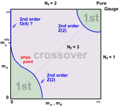
Figure 4: Schematic phase transition behavior of three flavor QCD for different choices of quark masses at zero density 1009.4089 .

FIG. 4 shows the schematic phase transition behavior of three flavor QCD for different choices of quark masses at $\mu=0$ 1009.4089 . We can see that, the order of the phase transition at $\mu=0$ depends on the quark masses. There are two limit regions where the phase transition is first order at $\mu=0$. One of them is near the chiral limit, i.e. $m_{u}=m_{d}=m_{s}=0$. The other is near the decoupling limit, i.e. $m_{u}=m_{d}=m_{s}\rightarrow\infty$. Thus there are two possibilities to interpret the phase diagram of our holographic QCD model.

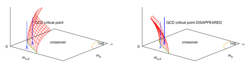
Figure 5: The chiral critical surfaces in the case of positive (left) and negative (right) curvature from lattice QCD 1009.4089 .

The first possibility is to interpret our result as for the light quarks (near the point of chiral limit) and the phase transition is the chiral symmetry breaking phase transition. For a not very large chemical potential $\mu$, lattice calculation shows that the chiral critical line separating the crossover from the first order phase transition regions expands as increasing the chemical potential $\mu$ to form a chiral critical surface. The sign of the curvature of the critical surface is crucial to determine the phase structure at finite $\mu$. In FIG. 5, the chiral critical surfaces in the case of positive and negative curvature are showed. In the interpretation of the light quarks, the mass point locates near the origin. The first order transition will be preserved for any finite $\mu$ if the curvature of the chiral critical surface is positive, while it will becomes a crossover at a finite chemical potential $\mu_{c}$ if the curvature of the chiral critical surface is negative. Recent lattice calculations shows that the curvature of the chiral critical surface is more like negative 0607017 ; 1009.4089 that is consistent with the phase diagram of our holographic QCD model.

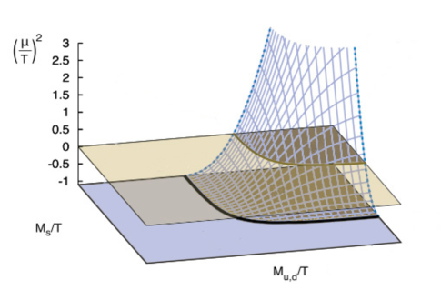
Figure 6: The deconfinement critical surface from lattice QCD 1111.4953 .

The other possibility is to interpret our result as for the heavy quarks (near the point of decoupling limit) and the phase transition is the deconfinement phase transition. Similar to the chiral critical line, lattice calculation shows that the deconfinement critical line separating the crossover from the first order phase transition regions expands as increasing the chemical potential $\mu$ to form a deconfinement critical surface. FIG. 6 shows the recent result of the deconfinement critical surface from lattice QCD 1111.4953 . In our interpretation of heavy quarks, the mass point locates near the infinite mass point. The first order phase transition at $\mu=0$ will becomes a crossover at a finite chemical potential $\mu_{c}$ and it is consistent with the phase diagram of our holographic QCD model. The phase transition for heavy quarks has been extensively studied recently by using lattice QCD method 1009.4089 ; 1011.4747 ; 1106.0974 ; 1111.4953 ; 1202.6113 ; 1207.3005 ; 1210.7994 .

Among the two possible interpretations of our holographic QCD model,  we will focus on the heavy quark interpretation in the rest of our paper. The reason is that, for the light quarks, the lattice QCD simulation has almost confirmed that the physical point of light quarks mass locates in the crossover region at zero chemical potential in FIG. 4. While for the heavy quarks, the lattice QCD does not give any constraint yet and the physical point of the heavy quarks mass has great possibility to locate in the first order region at zero chemical potential. Furthermore, if we re-examine the gravity side more carefully, we realize that we did not take into account the backreaction from the matter fields when we solved our gravitational background. We only consider the baryon number chemical potential, but not the dynamical quarks. This means that we are considering the quenched limit of the heavy quarks.

To interpret our result as for the heavy quarks with the deconfinement phase transition, there is still a problem in the gravity side. It is widely believed that the deconfinement phase transition in the field theory side is dual to the Hawking-Page phase transition in the gravity side. Hawking-Page phase transition is the transition between black hole and thermal gas backgrounds. However, in our gravity background, the phase transition is between a large black hole and a small black hole backgrounds for non-zero chemical potential. Thus it sounds inconsistent to consider that the black hole to black hole phase transition in the gravity side is dual to the deconfinement phase transition in QCD. Our resolution for this problem is that, although it is thermodynamically stable, the small black hole is dynamical unstable. On the other hand, the gauge group in realistic QCD is $SU\left(N\right)\sim SU\left(3\right)$. Thus we have to consider the finite $N$ effect in the gravity side. If we still require that the gravity limit held, this is merely to consider the finite string coupling constant by including the loop correction, i.e. the quantum effect. It is well-known that small black holes are quantum mechanically unstable and will quickly evaporate away by quantum radiation. Therefore, right after the phase transition of a large black hole to a small black hole, the small black hole will continue to evaporate away quickly to a thermal gas background. In this sense, the black hole to black hole phase transition can be interpreted as the deconfinement phase transition in the dual QCD theory.

In our heavy quarks interpretation, an important question is where the critical point is, i.e. the point where the first order phase transition cease to become a crossover in the phase diagram FIG. 3. Locating the critical point is a crucial job to understand the phase structure of QCD. As we have seen in FIG. 2, the critical point is the point where the self-intersection disappears. We thus obtain the critical point as $\left(\mu_{c},T_{c}\right)\simeq\left(0.714GeV,0.528GeV\right)$. To justify the critical point we got, we expand the the function $A_{t}\left(z\right)$ in Eq.(2.47) near the boundary $z\rightarrow 0$ as

$$A_{t}\left(z\right)=\mu\dfrac{e^{cz^{2}}-e^{cz_{H}^{2}}}{1-e^{cz_{H}^{2}}}=\mu+\dfrac{2c\mu}{1-e^{cz_{H}^{2}}}z^{2}+\cdots,$$ (3.14)

from which the baryon $\rho$ density can be read off as

$$\rho=-\dfrac{2c\mu}{1-e^{cz_{H}^{2}}}.$$ (3.15)

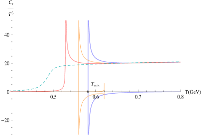
( a )                                                                 ( b )

Figure 7: (a) The baryon density $\rho$ v.s. the chemical potential $\mu$. The curve is single-valued for $T>T_{c}$, while it is multi-valued for $T<T_{c}$. At $T=T_{c}$, the slope becomes infinite at $\mu=\mu_{c}$. (b) The specific heat $C_{V}$ v.s. Temperature. The negative value of $C_{V}$ corresponds to the thermodynamically instability. For $\mu<\mu_{c}$, $C_{V}$ is negative for a range of $T$. For $\mu>\mu_{c}$, the specific heat is always positive implying no phase transition.

We plot the baryon density $\rho$ v.s. the chemical potential $\mu$ in (a) of FIG. 7. For $T<T_{c}$, the baryon density $\rho$ is single-valued which indicates that there is no phase transition. While for $T>T_{c},$ $\rho$ is multi-valued which indicates that there is a phase transition at certain value of the chemical potential $\mu$. At the critical temperature $T=T_{c}$, the slope of the $\rho-\mu$ curve becomes infinite at the critical chemical potential $\mu_{c}$. The behavior of the baryon number $\rho\left(\mu\right)$ near the critical temperature $T_{c}$ is consistent with the result we obtained from the free energy.

The susceptibility is defined as

$$\chi=\left(\dfrac{\partial\rho}{\partial\mu}\right)_{T},$$ (3.16)

which is just the slope in (a) of FIG. 7. For $T<T_{c}$, the susceptibility is always positive, $\chi>0$ implies that the black hole with any chemical potential value is thermodynamically stable. On the other hand, for $T<T_{c}$, $\chi$ could be negative for a range of $\mu$ where the black hole is thermodynamically unstable. At $T=T_{c}$, $\chi\rightarrow\infty$ at $\mu=\mu_{c}$ which indicates that a phase transition happens around there.

The similar behavior of the susceptibility $\chi$ can be seen from the plot of the specific heat $C_{V}$ v.s. the temperature $T$ in (b) of FIG. 7, where the specific heat $C_{V}$ is defined as

$$C_{V}=T\left(\dfrac{\partial s}{\partial T}\right)_{\mu}.$$ (3.17)

We note that, in the $C_{V}-T$ diagram, the negative value of the specific heat corresponds to the thermodynamically instability. For $\mu>\mu_{c}$, the specific heat is always positive, $C_{V}>0$ implies that the black hole with any temperature is thermodynamically stable. While for $0<\mu<\mu_{c}$, $C_{V}$ could be negative for a range of $T$ where the black hole is thermodynamically unstable. At $\mu=0$, there is a minimum temperature $T_{\min}$ for the black hole solutions where the specific heat diverges. The Hawking-Page like phase transition happens at a temperature slightly above $T_{\min}$ at $T_{HP}$.

III.3 Equations of State

The speed of sound is defined as

$$c_{s}^{2}=\dfrac{\partial\ln T}{\partial\ln s}.$$ (3.18)

Figure 8: The squared of speed of sound $c_{s}^{2}$ v.s. temperature. For $\mu<\mu_{c}$, $c_{s}^{2}$ is negative for a range of $T$ implying dynamical instability and there is a phase transition. For $\mu>\mu_{c}$, $c_{s}^{2}$ becomes smooth and always positive. At $\mu=\mu_{c}$, $c_{s}^{2}$ touches the $x$-axis at $T=T_{c}$ where the phase transition transfers to a crossover.

FIG. 8 plots the squared of speed of sound $c_{s}^{2}$ v.s. the temperature $T$. For $0<\mu<\mu_{c}$, the speed of sound is imaginary for a range of temperature, indicating a Gregory-Laflamme instability 9301052 ; 9404071 . This is related to the general version of Gubser-Mitra conjecture 0009126 ; 0011127 ; 0104071 , i.e. the dynamical stability of a horizon is equivalent to the thermodynamic stability. In our system, the negative specific heat implies thermodynamically unstable. While the imaginary speed of sound implies the amplitude of the fixed momentum sound wave would increase exponentially with time, reflecting the dynamical instability. Roughly speaking, $C_{V}<0$ is equivalent to $c_{s}^{2}<0$ in our system. For $\mu>\mu_{c}$, the speed of sound behaves as a sharp but smooth crossover. At the critical point $\mu=\mu_{c}$, a second order phase transition happens where $c_{s}^{2}$ goes to $0$ at the critical temperature $T_{c}$ but never becomes negative. In all the case, $c_{s}^{2}$ approaches the comformal limit $1/3$ at very high temperature as expected.

We plot other equations of state in FIG. 9. The entropy of our black hole solution has been calculated in (3.8) and is plotted in (a) of FIG. 9. At $\mu=0$, there is a minimum temperature $T_{\min}$ for the black hole solutions. The black hole solutions with very low entropy and high temperature always have negative specific heat and are thermodynamically unstable and the black hole will transit to the thermal gas through a Hawking-Page phase transition. For $0<\mu<\mu_{c}$, the entropy is multi-valued for a region of temperature which indicates a phase transition between high entropy and low entropy black holes. For $\mu\geq\mu_{c}$, the entropy is single-valued and there is no phase transition. The similar phase behaviors have been discussed in 0804.0434 for a holographic QCD model with different values of parameters tuned by hand.

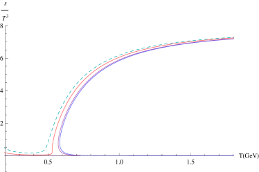
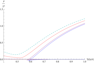
( a )                                                         ( b )

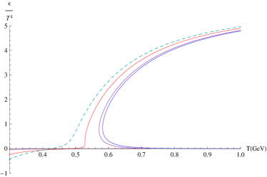
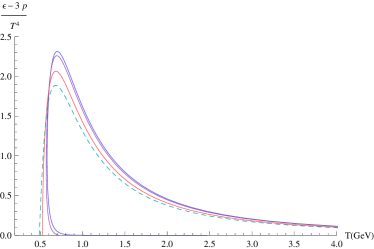
( c)                                                         ( d )

Figure 9: (a) The entropy $s$ v.s. temperature. (b) The pressure $p$ v.s. temperature. (c)The energy $\epsilon$ v.s. temperature. (d) The trace anomaly $\epsilon-3p$ v.s. temperature.

The pressure $p$ and the energy $\epsilon$ can be calculated from the free energy as

$$p=-F\text{, \ \ }\epsilon=F+sT.$$ (3.19)

(b) and (c) of FIG. 9 plot the pressure $p$ and the energy $\epsilon$ v.s. temperature $T$. For some particular $\mu$ and $T$, the pressure becomes negative which seems not make sense for a real physical system. However, we see that the pressures for all the thermodynamically favorite backgrounds are always positive. Both the pressure and the energy increase with the chemical potential, that pushes the phase transition temperature $T_{BB}$ to the smaller values for growing $\mu$. Our results are consistent to the recent lattice results with finite chemical potential 1204.6710 .

We finally plot the trace anomaly $\epsilon-3p$ v.s $T$ in (d) of FIG. 9. At $\mu=0$, the sharp peak with a infinite slope edge indicates a phase transition. With the growing chemical potential $\mu$, the peak becomes wider with decreasing height. The phase transition turns to be weaker and weaker for increasing $\mu$ and eventually becomes a crossover.

IV Conclusion

In this paper, we studied the Einstein-Maxwell-dilaton system. We obtained a family of analytic black hole solutions by the potential reconstruction method. We then studied the thermodynamic properties of the black hole backgrounds. We computed the free energy to get the phase diagram of the black hole backgrounds. In its dual holographic QCD theory, we are able to realized the Regge trajectory of the vector mass spectrum by fixing the gauge kinetic function. We then discussed the possible interpretations of the phase structure that we obtained from the gravitational background by comparing the lattice QCD simulations. We argued that the heavy quarks interpretation is more favored in our system. We calculated the equations of state in our holographic QCD model. We found that our dynamical model captures many properties in the realistic QCD. The most remarkable feature of our model is that, by changing the chemical potential, we are able to see the conversion from the phase transition to a crossover dynamically. We identified the critical point in our holographic QCD model and calculated its value. As the authors knowledge, our model is the first holographic QCD model which could both dynamically describe the transformation from the phase transition to the crossover by changing the chemical potential and realize the linear Regge trajectory for the meson spectrum.

Since we interpret our holographic QCD model as a heavy quarks system, it would be interesting to perform a lattice simulation on the equations of state of a heavy quarks system and compare with our results. On the other hamd, there are many future directions one can study. For example, the most interesting issue is to find an appropriate warped factor such that one can obtain a phase diagram similar to the common QCD phase diagram. Another interesting issue is to incorporate the chiral symmetry breaking by introducing a scalar coupled to the flavor fields and take the backreactions of flavor fields into account. It is also interesting to compute the linear quark-antiquark potential and expectation value of Polykov loop. One can compute the meson spectrum and determine the quarkonium dissociation temperature in our background. One can also compute the various transport coefficients like shear visocisty, bulk viscosity and so on. It is also interesting to compute the critical exponents of various physical quantities near the critical point. Some of these issues are in progress.

- (1) O. Philipsen, “Lattice QCD at non-zero temperature and baryon density,” arXiv:1009.4089 [hep-lat].
- (2) J. Babington, J. Erdmenger, N. J. Evans, Z. Guralnik and I. Kirsch, “Chiral symmetry breaking and pions in nonsupersymmetric gauge / gravity duals,” Phys. Rev. D 69, 066007 (2004) [hep-th/0306018].
- (3) M. Kruczenski, D. Mateos, R. C. Myers and D. J. Winters, “Towards a holographic dual of large N(c) QCD,” JHEP 0405, 041 (2004) [hep-th/0311270].
- (4) M. Kruczenski, D. Mateos, R. C. Myers and D. J. Winters, “Meson spectroscopy in AdS / CFT with flavor,” JHEP 0307, 049 (2003) [hep-th/0304032].
- (5) S. Kobayashi, D. Mateos, S. Matsuura, R. C. Myers and R. M. Thomson, “Holographic phase transitions at finite baryon density,” JHEP 0702, 016 (2007) [hep-th/0611099].
- (6) T. Sakai and S. Sugimoto, “Low energy hadron physics in holographic QCD,” Prog. Theor. Phys. 113, 843 (2005) [hep-th/0412141].
- (7) T. Sakai and S. Sugimoto, “More on a holographic dual of QCD,” Prog. Theor. Phys. 114, 1083 (2005) [hep-th/0507073].
- (8) J. Erlich, E. Katz, D. T. Son and M. A. Stephanov, “QCD and a holographic model of hadrons,” Phys. Rev. Lett. 95, 261602 (2005) [hep-ph/0501128].
- (9) A. Karch, E. Katz, D. T. Son and M. A. Stephanov, “Linear confinement and AdS/QCD,” Phys. Rev. D 74, 015005 (2006) [hep-ph/0602229].
- (10) B. Batell and T. Gherghetta, “Dynamical Soft-Wall AdS/QCD,” Phys. Rev. D 78, 026002 (2008) [arXiv:0801.4383 [hep-ph]].
- (11) W. de Paula, T. Frederico, H. Forkel and M. Beyer, “Dynamical AdS/QCD with area-law confinement and linear Regge trajectories,” Phys. Rev. D 79, 075019 (2009) [arXiv:0806.3830 [hep-ph]].
- (12) S. S. Gubser and A. Nellore, “Mimicking the QCD equation of state with a dual black hole,” Phys. Rev. D 78, 086007 (2008) [arXiv:0804.0434 [hep-th]].
- (13) U. Gursoy, E. Kiritsis, L. Mazzanti, G. Michalogiorgakis and F. Nitti, “Improved Holographic QCD,” Lect. Notes Phys. 828, 79 (2011) [arXiv:1006.5461 [hep-th]].
- (14) O. DeWolfe, S. S. Gubser and C. Rosen, “A holographic critical point,” Phys. Rev. D 83, 086005 (2011) [arXiv:1012.1864 [hep-th]].
- (15) O. DeWolfe, S. S. Gubser and C. Rosen, “Dynamic critical phenomena at a holographic critical point,” Phys. Rev. D 84, 126014 (2011) [arXiv:1108.2029 [hep-th]].
- (16) R. -G. Cai, S. He and D. Li, “A hQCD model and its phase diagram in Einstein-Maxwell-Dilaton system,” JHEP 1203, 033 (2012) [arXiv:1201.0820 [hep-th]].
- (17) D. Li, S. He, M. Huang and Q. -S. Yan, “Thermodynamics of deformed AdS5 model with a positive/negative quadratic correction in graviton-dilaton system,” JHEP 1109, 041 (2011) [arXiv:1103.5389 [hep-th]].
- (18) R. -G. Cai, S. Chakrabortty, S. He and L. Li, “Some aspects of QGP phase in a hQCD model,” arXiv:1209.4512 [hep-th].
- (19) M. Shifman, “Highly excited hadrons in QCD and beyond,” hep-ph/0507246.
- (20) C. Park, D. -Y. Gwak, B. -H. Lee, Y. Ko and S. Shin, “The Soft Wall Model in the Hadronic Medium,” Phys. Rev. D 84, 046007 (2011) [arXiv:1104.4182 [hep-th]].
- (21) Y. Kim, J. -P. Lee and S. H. Lee, “Heavy quarkonium in a holographic QCD model,” Phys. Rev. D 75, 114008 (2007) [hep-ph/0703172 [HEP-PH]].
- (22) M. Fujita, K. Fukushima, T. Misumi and M. Murata, “Finite-temperature spectral function of the vector mesons in an AdS/QCD model,” Phys. Rev. D 80, 035001 (2009) [arXiv:0903.2316 [hep-ph]].
- (23) M. Fujita, T. Kikuchi, K. Fukushima, T. Misumi and M. Murata, “Melting Spectral Functions of the Scalar and Vector Mesons in a Holographic QCD Model,” Phys. Rev. D 81, 065024 (2010) [arXiv:0911.2298 [hep-ph]].
- (24) L. -X. Cui, S. Takeuchi and Y. -L. Wu, “Quark Number Susceptibility and QCD Phase Transition in the Predictive Soft-wall AdS/QCD Model with Finite Temperature,” Phys. Rev. D 84, 076004 (2011) [arXiv:1107.2738 [hep-ph]].
- (25) L. -X. Cui, S. Takeuchi and Y. -L. Wu, “Thermal Mass Spectra of Vector and Axial-Vector Mesons in Predictive Soft-Wall AdS/QCD Model,” JHEP 1204, 144 (2012) [arXiv:1112.5923 [hep-ph]].
- (26) F. Giannuzzi, “Holographic vector mesons in a hot and dense medium,” arXiv:1209.4198 [hep-ph].
- (27) U. Gursoy, E. Kiritsis, L. Mazzanti and F. Nitti, “Holography and Thermodynamics of 5D Dilaton-gravity,” JHEP 0905, 033 (2009) [arXiv:0812.0792 [hep-th]].
- (28) M. Fromm, J. Langelage, S. Lottini and O. Philipsen, “The QCD deconfinement transition for heavy quarks and all baryon chemical potentials,” JHEP 1201, 042 (2012) [arXiv:1111.4953 [hep-lat]].
- (29) P. de Forcrand and O. Philipsen, “The Chiral critical line of N(f) = 2+1 QCD at zero and non-zero baryon density,” JHEP 0701, 077 (2007) [hep-lat/0607017].
- (30) H. Saito et al. [WHOT-QCD Collaboration], “The order of the deconfinement phase transition in a heavy quark mass region,” PoS LATTICE 2010, 212 (2010) [arXiv:1011.4747 [hep-lat]].
- (31) H. Saito et al. [WHOT-QCD Collaboration], “Phase structure of finite temperature QCD in the heavy quark region,” Phys. Rev. D 84, 054502 (2011) [Erratum-ibid. D 85, 079902 (2012)] [arXiv:1106.0974 [hep-lat]].
- (32) H. Saito et al. [WHOT-QCD Collaboration], “Finite density QCD phase transition in the heavy quark region,” PoS LATTICE 2011, 214 (2011) [arXiv:1202.6113 [hep-lat]].
- (33) M. Fromm, J. Langelage, S. Lottini, M. Neuman and O. Philipsen, “The silver blaze property for QCD with heavy quarks from the lattice,” arXiv:1207.3005 [hep-lat].
- (34) M. Fromm, J. Langelage, S. Lottini, M. Neuman and O. Philipsen, “Phase transitions in heavy-quark QCD from an effective theory,” arXiv:1210.7994 [hep-lat].
- (35) R. Gregory and R. Laflamme, “Black strings and p-branes are unstable,” Phys. Rev. Lett. 70, 2837 (1993) [hep-th/9301052].
- (36) R. Gregory and R. Laflamme, “The Instability of charged black strings and p-branes,” Nucl. Phys. B 428, 399 (1994) [hep-th/9404071].
- (37) S. S. Gubser and I. Mitra, “Instability of charged black holes in Anti-de Sitter space,” hep-th/0009126.
- (38) S. S. Gubser and I. Mitra, “The Evolution of unstable black holes in anti-de Sitter space,” JHEP 0108, 018 (2001) [hep-th/0011127].
- (39) H. S. Reall, “Classical and thermodynamic stability of black branes,” Phys. Rev. D 64, 044005 (2001) [hep-th/0104071].
- (40) S. .Borsanyi, G. Endrodi, Z. Fodor, S. D. Katz, S. Krieg, C. Ratti and K. K. Szabo, “QCD equation of state at nonzero chemical potential: continuum results with physical quark masses at order ,” JHEP 1208, 053 (2012) [arXiv:1204.6710 [hep-lat]].