Photo-mechanical energy conversion using polymer brush dissociation

Abstract

A device is investigated that continuously and directly converts light into mechanical energy, using polymers and photodissociation. A polymer brush tethered to a surface, is brought into contact with a parallel plate a small distance above it that contains reaction sites where photodissociation of bound polymer and light can occur. Under the appropriate conditions, the collective effect of these polymers is to apply a force parallel to the plates, converting incoming light into mechanical work. Numerical work is carried out to understand this effect, a three dimensional Langevin simulation, solution to the Fokker Planck equation, and a one dimensional Monte Carlo simulation. Theoretical analysis of the Fokker Planck equation is used to study a model where equilibration of the unbound state occurs and equilibration to a metastable equilibrium is achieved in the bound state. It is shown that the work per cycle can be made much larger than the thermal energy but at the expense of requiring a greatly diminished photodissociation rate. Parameters are discussed in order optimize mechanical energy conversion.

I Introduction

There are many proposals to convert light into mechanical energy using smart polymeric photo-responsive materials IrieKunwatchakun ; Irie ; SuzukiHirasa ; BehlLendlein ; RoyGupta or the synthesis of individual molecules that lead to rotary or linear motion credi2006 .

Photoresponsive materials use a conformational change of a macroscopic collection of polymers in response to light or an external change in temperature and pH. This will cause a change in volume. If this process is reversible, which it is in many instances, this device can be cycled to derive mechanical energy IrieKunwatchakun ; Irie ; SuzukiHirasa .

In general, there are many scenarios leading to a change in configuration of a molecule in response to light Irie : cis-trans isomerization, zwitter ion formation, radical formation, ionic dissociation, and ring formation/cleavage. If such light-sensitive elements are incorporated into a macromolecular system, this can in principle, through thermodynamic cycles, to conversion of light to mechanical power.

Remarkable advances in the design of molecules have led to prototypes for light-driven synthetic molecular motors credi2006 . Many of these are based on photoisomerization reactions that enable rotary motion of molecules when combined with thermal rotation steps terWiel2005 ; Ruangsupapichat ; Vicario ; credi2006 . It has also been possible to make threading-dethreading systems Ashton1998 ; credi2006 , and shuttle molecular rings Ashton2000 ; credi2006 . There has even been progress on a macroscopic level, such as creating droplet motion by modifying surface properties Berna or inducing mechanical deformation Liu similar to what is achieved with photo-responsive materials IrieKunwatchakun ; Irie ; SuzukiHirasa ; BehlLendlein ; RoyGupta .

Much of the research in this area is inspired by biological machines such as myosin II that work by quite a different principle than man-made macroscopic motors BustamanteKellerOster . Biological motors use chemical energy rather than photons to produce mechanical power however this difference does not affect the basic mechanism of operation. A myosin head can be thought of as being in two states, bound or unbound. Thermal noise in the unbound state can cause the head to bind to actin, producing a force. The hydrolysis of ATP releases energy causing the head to return to the unbound state. The biochemistry of a real motor protein is considerably more complicated, but by simplifying this description to one involving only these two states, the motion can be analyzed, and it is easily seen that electromagnetic energy can be used instead of chemical energy ProstPRL .

In this paper, I investigate the use of photons in powering a two state motor system similar to biological motors. I consider creating motion between two surfaces that are very close together by placing an asymmetric polymer brush between them. This could potentially have advantages. A continuous source of light would create a motion that is constant on a macroscopic scale, that could for example, rotate the surfaces relative to each other. It would not require any additional mechanisms to keep it moving, other than the microscopic motion of molecules between the plates.

The device proposed here falls into a distinct category different than the experimental approaches above. It is not a macroscopic smart material that changes properties in response to external stimuli. The device described in the next section works on the scale of an individual polymers, and the force generated on the surfaces is the sum of these molecules acting independently of each other. However it is unlike the chemical synthesis approach that requires different states of isomerization. The principles that it relies on are robust and just require photodissociation of polymer to a binding site, and, as in the case of biological motors, some degree of asymmetry. This asymmetry, plus a disruption of thermal equilibrium due to energy input are the two factors needed to convert energy from chemical or electromagnetic energy, to mechanical ProstPRL .

The paper is organized as follows. In Sec. II the photo-mechanical system is described and rough estimates of its operation are given in Sec. III including a discussion of its potential efficiency. In order to illustrate the characteristics that need to be understood, a three dimensional simulation of this device is carried out In Sec. IV. At this point the physics of this system is investigated in more detail, starting with general considerations, in Sec. V of its steady state behavior using Fokker Planck equations. The results will be used in subsequent sections. An exact description of this system is possible in steady state and the resulting differential equation is solved numerically in one dimension in Sec. VI. This allows to understand better how effective the asymmetry in the force produces power, and influences the direction that is taken in the rest of this work. Sec. VII studies a useful limit that is hard to probe numerically, but allows to understand how the efficiency of this system is related to spring stiffness, metastability, relaxation times, and the photo-dissociation rate. We then use this model to understand the efficiency, Sec. VII.1 using a one dimensional Monte Carlo model that is in this regime. Finally in Sec. VIII we conclude on how the physics that has been learned might be useful in optimizing experimental parameters for such a system.

II The System

The components needed to do constant photomechanical energy conversion are are illustrated in Fig. 1.

• A flat plate of semi-flexible polymer brushes. Polymer brushes are polymers, each with one end tethered to a wall in a suitable solvent.

• A parallel plate right above the brush. These polymers are put in contact with a parallel plate close to the surface so that their ends are able to interact with it.

• The parallel plate contains an array of photoreactive binding sites. It is crucial that these polymers bind with the surface in an asymmetric way, so that the average binding orientation of each is the same, and not perpendicular to the plate.

• At least one of the plates is transparent. Light causes the unbinding of polymer ends from the photoreactive binding sites.

• Binding catalyst. To control the rate at which binding occurs, the binding of the end of the polymer to a binding site can be facilitated by the use of a catalyst. The concentration of the catalyst can be used to control the rate of binding.

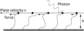
(a) (b)

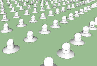
Figure 1: (a) A schematic of the light energy to mechanical converter. A polymer brush of semiflexible chains is put in contact with a plate a height $h$ above the base, containing an array of anisotropic binding sites. Polymer ends are trapped by unlikely thermal fluctuations, applying a non-zero average force parallel to the plate. Photodissociation of the polymer ends with the binding sites releases the chain end that will move until it finds another site. The upper plate moves at a velocity $\rm v$, thereby generating power. A single track is shown, and the separation between binding sites is $L$. (b) A three dimensional sketch of the binding sites. The binding of the polymer ends (not shown) takes place on the oval surfaces protruding from the plate, and do so in an asymmetric manner. The sites are organized into one dimensional tracks, where the distance between tracks need not be the same as $L$ in (a).

In most of the discussion below, the polymers can be considered to be separated from each other by a sufficient distance so that we can ignore inter-chain interactions. The absorption of light causing unbinding will happen asynchronously. The ends tethered to the lower plates are at positions that are either random or incommensurate with the binding sites of the upper plate. Altogether this means that the motion of each polymer is uncorrelated with the others in the system.

The total effect of the forces acting on the plates can be used to perform work against a force acting on the upper plate. Because we assume that the number of polymers contributing is very large and are asynchronous, the net velocity of the upper plate $v$ will be constant, as will be the net force acting on the plate.

In the following we will analyze the system and model it in different ways to better understand the power generation.

III Estimate of system parameters

We will now make a crude estimate with realistic parameters, how well this device should work. We envisage separate one dimensional tracks of the kind shown in Fig. 1(b). The spacing between the tracks could be greater than the distances between polymers on a single track. In reality, it might prove more efficacious to manufacture a square array of polymers and binding sites but we will allow two separate length scales in our analysis below.

We will assume a solar intensity of $I=600W/m^{2}$, and an average photon energy of $e=2eV$. We will take the relaxation time of a polymer to be $\tau=10^{-7}s$, which corresponds roughly to a polymer size of $3nm$. The number of unbinding events, if every photon was absorbed at a binding site, is $I/e\approx 2\times 10^{21}/(m^{2}s)$. If the density of polymers is $\sigma$, then for all of these events to be utilized requires $I/e=\sigma/\tau$, or $\sigma=2\times 10^{14}/m^{2}$, which is a separation of $1/\sqrt{\sigma}\approx 70nm$. The amount of energy per step that is gained by a photo-dissociation event is of order $k_{B}T$. With such parameters, this is expected to yield an efficiency of order $1\%$. However, as we will show below, longer relaxation times allow for more energy per step, and this requires a higher polymer density. However the two dimensional density is limited by inter-chain interactions. In the case considered here, this density could be increased roughly by three orders of magnitude. However the relaxation time for this system depends exponentially on the force generated, so a three order of magnitude increase in relaxation time would only increase the efficiency by a factor of about $7$ furthermore, the detailed analysis presented below suggests that with optimal conditions, the efficiency of conversion is about $7\%$. To increase the efficiency of solar conversion further might require stacking devices.

There are other means of increasing the solar conversion efficiency by first converting solar radiation to lower energy photons. For example, two methods for doing this are fluorescent down-conversion of solar photons Klampfatis , or thermophotovoltaic down-conversion Harder .

Further speculation on device efficiency is premature as there will undoubtedly be many unforeseen technical problems that will likely provide other obstacles to increasing device efficiency. However an efficiency for direct photo-mechanical conversion of about $7\%$ is still a useful amount of power comparable to photovoltaic conversion with amorphous solar cells, and also because power is lost in electro-mechanical conversion, which is not a problem with direct mechanical energy conversion.

IV Three dimensional model

We start by simulating a three dimensional model of this system. There are two components to the system, the polymer and the binding sites. The polymer chain is modeled as having $N$ links of fixed length, and is semiflexible with chain stiffness $K$. Denote the coordinates of the $ith$ bead as ${\bf r}_{i}$. The elastic potential for the middle of the chain for the $ith$ bead is

$$U_{E}(i)\equiv-\frac{C}{2}(|{\bf r}_{i+2}-{\bf r}_{i}|^{2}+|{\bf r}_{i-2}-{\bf r}_{i}|^{2})$$ (1)

where $C$ is the elastic constant.

The binding potential of the polymer has two components, an isotropic component $U_{i}$ and directional component $U_{d}$. $U_{i}(r)$ is short range with a length scale $r_{s}$ and scale $V_{a}$

$$U_{i}(r)\equiv-\frac{V_{a}}{8}(r_{s}^{2}-r^{2})^{4}$$ (2)

and $U_{d}$ uses a direction ${\bf\hat{n}}_{a}$ so that the difference between the last two end beads ${\Delta{\bf r}}={\bf r}_{1}-{\bf r}_{0}$ will give a minimum in $U_{d}$ along that direction

$$U_{d}({\bf r}_{0},{\bf r}_{1})\equiv(\bigl{|}\frac{{\Delta{\bf r}}-{\bf\hat{n}}_{a}}{|{\Delta{\bf r}}-{\bf\hat{n}}_{a}|}\bigr{|}^{2}+1)U_{i}(r).$$ (3)

The end attached to the lower surface is always bound. The other end can bind to a periodic linear array of binding sites equally spaced at a distance $L$.

There are two states that the system can be in, unbound, $0$, and bound $1$. There are two parameters that control binding, the rate at which dissociation occurs $c_{0}$, and the rate that dissociated ends can be rebound $c_{1}$.

The distance between the lower and upper surface is $h$ and their relative velocity is $\rm v$.

The model was simulated with a Langevin equation, at finite temperature $T$. Although inertial effects are typically small at these microscopic scales, it was included for completeness. An algorithm was used that efficiently updates this system with fixed link lengths DeutschCerfFriction .

The simulation was run to determine how the force and power generated are influenced by the plate velocity. Fig. 2 shows the results of four simulations with different values of $c_{0}$ and $c_{1}$. The parameters used were: $4$ links, $h=1$, spacing between binding sites $L=2$, the direction of ${\bf\hat{n}}_{a}$, is $\pi/4$, $V_{a}=30$, link length of $1$, particle mass of $1$, $C=1.5$, $r_{s}=2.0$, and a coefficient of damping of $10$.

The force generated is highest approaching zero velocity and decreases until it becomes negative, at which point it is taking mechanical energy to move it at such high speeds. Qualitatively, this is the point where frictional drag dominates over photo-energy conversion.

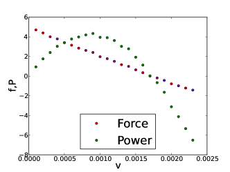
(a) (b)

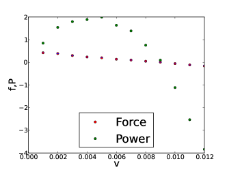
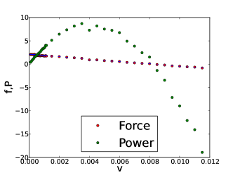
(c) (d)

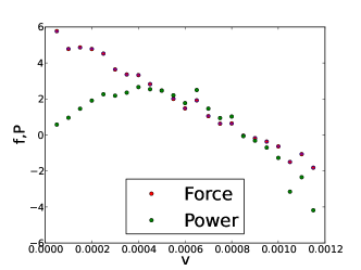
Figure 2: The average force $f$ and the power $P=f{\rm v}$ measured as a function of the relative velocity between the plates $\rm v$. For clarity, the power is multiplied by $2000$. There were $4$ links, with a plate separation of $h=1$, spacing between binding sites $L=2$, the direction of ${\bf\hat{n}}_{a}$, that is, the binding angle is $\pi/4$, $V_{a}=30$, link length of $1$, and elastic constant $C=1.5$, potential range $r_{s}=2.0$, and a coefficient of damping of $10$. (a) the rate of dissociation $c_{0}=0.01$, rate of rebinding $c_{1}=0.05$. (b) $c_{0}=0.05$, $c_{1}=0.01$ (c) $c_{0}=0.05$, $c_{1}=0.05$ (d) $c_{0}=0.005$, $c_{1}=0.05$

Note that the highest power $P=f{\rm v}$ is seen for $c_{0}=c_{1}=0.05$. The force extrapolated to ${\rm v}=0$ is $f=2.07$ and is about three times less than the force seen in Fig. 2(b) where $c_{0}=0.05$ and $c_{0}=0.01$.

Higher maxima in the power are generally seen with increasing $c_{0}$ and $c_{1}$. As an example, the simulation was run for small elastic constant $C=0.5$, at different values of $c_{0}$ and $c_{1}$, but with all other parameters the same as above. This higher power is still at the expense of efficiency, as higher dissociation rates imply a higher photon flux.

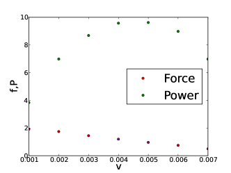
(a) (b)

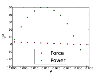
Figure 3: The average force $f$ and the power $P=f{\rm v}$ measured as a function of the relative velocity between the plates $\rm v$. The same parameters and scaling are used as in Fig. 2 except $C=0.5$ and (a) $c_{0}=c_{1}=0.05$, and (b) $c_{0}=c_{1}=0.4$. Higher maximum power is seen for larger unbinding rates.

V Steady State Probability Distribution

To understand the above simulation in more detail, requires a better understanding of the mechanisms involved. There have been a very large number of works on the theory of motor proteins ReimannRev ; BustamanteKellerOster , and we will follow the two state approach mentioned above of Prost et. al. ProstPRL ; JulicherRevModPhys . The major difference is that they considered the two states to be periodic potentials, whereas here we model the system to more closely mimic the particular device we are investigating allowing the exploration of force versus velocity. Hence instead of considering the position of a particle moving between two periodic potentials, we consider the unbound state to have a free end described as moving in a bound potential around the tether point. Likewise, because of this tethering, the bound state potential is not periodic but has a periodic component as we will describe in detail below. Here we consider the probability distribution for this system in steady state, which is described by a Fokker Planck equation.

Initially to calculate the power that is produced, we will concentrate on the low velocity limit, with the two plates moving so slowly that this motion does not affect chain conformations appreciably. In this way, we can consider the average force exerted between the plates by a polymer in steady state in the limit ${\rm v}=0$ so that the tether point is not moving. It is most convenient to let the point at which the polymer is tethered to the bottom plate be a variable parameter ${\bf r}^{\prime}=x^{\prime}{{\bf\hat{x}}}$. With this point fixed, we consider the distribution of the other end of the polymer ${\bf r}$. We will assume that the internal dynamics of the chain chain are much faster than the binding and unbinding rates, so that the only degrees of freedom are ${\bf r}$, and if the polymer is bound, $i=0$ is unbound and $i=1$ is bound. Therefore the probability distribution of the system can be described by a function $P_{s}({\bf r};{\bf r}^{\prime})$. The equations describing this are ProstPRL

$$\partial_{t}P_{0}({\bf r})=\nabla\cdot(\nabla-{\bf f}_{0})P_{0}({\bf r})-c_{0}P_{0}({\bf r})+c_{1}P_{1}({\bf r})$$ (4a)

$$\partial_{t}P_{1}({\bf r})=\nabla\cdot(\nabla-{\bf f}_{1})P_{1}({\bf r})+c_{0}P_{0}({\bf r})-c_{1}P_{1}({\bf r})$$ (4b)

where the last ${\bf r}^{\prime}$ argument of $P$ has been left out for notational simplicity. The units here absorb the diffusion coefficient $D$ together with the time, that is $t$ as used here and below is really $D$ times the time. The force terms have absorbed a temperature factor $T$, that is ${\bf f}_{i}$, is really the force times $1/k_{B}T$. Those forces, ${\bf f}_{0}$ and ${\bf f}_{1}$ are the total forces acting on the upper end of the chain. When the system it is unbound is the force of a (possibly) nonlinear spring

$${\bf f}_{0}={\bf f}_{s}({\bf r}-{\bf r}^{\prime}).$$ (5)

When the system is bound we have total force is the sum of the spring force and a periodic force representing the binding potential

$${\bf f}_{1}={\bf f}_{s}({\bf r}-{\bf r}^{\prime})+{\bf f}_{p}({\bf r}).$$ (6)

These forces are assumed to be conservative, ${\bf f}_{s}$ and ${\bf f}_{p}$ are derived from potentials that respectively are $V_{s}$ and $V_{p}$.

In steady state the left hand sides of these equations are zero. We can eliminate the last two terms on the right hand side to obtain.

$$\hat{O}_{0}P_{0}+\hat{O}_{1}P_{1}=0$$ (7)

where

$$\hat{O}_{i}=\nabla\cdot(\nabla-{\bf f}_{i}),~{}~{}~{}i=0,1.$$ (8)

We can now calculate the average force exerted by the two potentials, is zero. In steady state, we multiply Eq. 7 by $x$ and integrate with respect to $x$, $y$ and $z$. Then using integration by parts, we have boundary terms at infinity. Because we are assuming that the spring potential grows without bounds, this confines $P_{0}$, and $P_{1}$, to a neighborhood around ${\bf r}^{\prime}$, so that the boundary terms vanish. We are then left with

$$\langle{\bf f}\rangle=\int({\bf f}_{0}P_{0}+{\bf f}_{1}P_{1})d^{d}{\bf r}=0$$ (9)

as is expected because $r$ is confined to a region of space so that the average velocity, and hence average force, will be zero.

We can also determine the total fraction of time spent in the bound or unbound states in steady state. First, because the probability of being in any state is unity,

$$\int(P_{0}({\bf r})+P_{1}({\bf r}))d^{d}{\bf r}=1.$$ (10)

Then by integrating Eq. 4a over all space, the derivative term integrates to 0, giving

$$\int(-c_{0}P_{0}({\bf r})+c_{1}P_{1}({\bf r}))d^{d}{\bf r}=0$$ (11)

hence

$$\int P_{0}({\bf r})d^{d}{\bf r}=\frac{c_{1}}{c_{0}+c_{1}},~{}~{}~{}\int P_{1}({\bf r})d^{d}{\bf r}=\frac{c_{0}}{c_{0}+c_{1}}.$$ (12)

To obtain the power produced by this device, we are not interested in the total force acting on the upper chain end because this includes the binding potential, but the average force due to the spring acting on the lower plate $\langle f_{s}\rangle$. We would like to calculate the work done in moving the lower point ${\bf r}^{\prime}$ by one period of ${\bf f}_{p}$. After moving one period the system is statistically identical to its starting point, and this method can therefore give the work done in moving $n$ such periods. Denoting the period of ${\bf f}_{p}$ by $L$, we would like to calculate

$$W_{l} =\int_{0}^{L}{\bf\hat{x}}\cdot\langle{\bf f}_{s}\rangle dx^{\prime}$$

$$=\int_{0}^{L}\int{\bf\hat{x}}\cdot{\bf f}_{s}({\bf r},x^{\prime}{\bf\hat{x}})(P_{0}({\bf r},x^{\prime}{\bf\hat{x}})+P_{1}({\bf r},x^{\prime}{\bf\hat{x}}))d^{3}{\bf r}dx^{\prime}$$ (13)

and using Eq. 9

$$W_{l}=-\int_{0}^{L}\int{\bf\hat{x}}\cdot{\bf f}_{p}({\bf r})P_{1}({\bf r},x^{\prime}{\bf\hat{x}})d^{3}{\bf r}dx^{\prime}.$$ (14)

In thermal equilibrium, where the transition rates $c_{0}$ and $c_{1}$ are both zero, we recover the Gibbs distribution. Let us assume, that the system starts, and therefore remains in state $i=1$. Then

$$P_{0}({\bf r},{\bf r}^{\prime})d^{3}{\bf r}=\frac{e^{-V_{1}}}{Z}d^{3}{\bf r}$$ (15)

where the partition function

$$Z({\bf r}^{\prime})=\int e^{-V_{1}}d^{3}{\bf r}$$ (16)

which will also have periodicity of $L$. In this case $W_{L}$ can be easily calculated because $P_{0}=0$ and $f_{s}=-\nabla V_{s}({\bf r}-{\bf r}^{\prime})=\nabla^{\prime}V_{s}({\bf r}-{\bf r}^{\prime})$. So

$$W_{L} = \int_{0}^{L}\int(\partial_{x^{\prime}}V_{s}({\bf r},x^{\prime}{\bf\hat{x}}))\frac{e^{-(V_{s}({\bf r}-{\bf\hat{x}}x^{\prime})+V_{p}({\bf r}))}}{Z(x^{\prime})}d^{3}{\bf r}dx^{\prime}$$ (17)

$$= -T(\log Z(L)-\log Z(0))=0$$

as it must be by the second law of thermodynamics.

VI One dimensional solution

In order to investigate how the power conversion depends on the forces acting on this system, it is important to simplify the three dimensional model to obtain a minimal model that depends on far fewer parameters. Therefore we investigate this model in one dimension.

A key point to understand is how asymmetry in the form of the force produces power. With symmetric spring and binding potentials, it is easily seem by symmetry, that no net power can be produced from this system. We now ask how asymmetry affects the results. We will see that even with a large asymmetry in the spring potential, the work defined by Eq. V is very small. Simulations using Monte Carlo or Langevin equations are too noisy to provide good estimates. We therefore instead use a more analytical approach.

The coupled Focker Planck Eqs. 4 (a) and (b) can be solved to produce an equation only involving one distribution function, $P_{0}$ in steady state. Using the definitions in Eq. 8, we can eliminate $P_{1}$.

$$(\hat{O}_{1}\hat{O}_{0}-c_{1}\hat{O}_{0}-c_{0}\hat{O}_{1})P_{0}=0$$ (18)

which is a fourth order equation in spatial variables.

Now we restrict the analysis to one dimension. In this case, $\hat{O}_{i}=\partial_{x}(\partial_{x}-f_{i})$ so we can integrate with respect to $x$. We note that because the spring confines $P_{0}$ to a localized region, it will go to zero as $x\rightarrow\pm\infty$. Therefore the integration constant must also be zero

$$((\partial_{x}-f_{1})\partial_{x}(\partial_{x}-f_{0})-c_{1}(\partial_{x}-f_{0})-c_{0}(\partial_{x}-f_{1}))P_{0}=0$$ (19)

which is a third order linear differential equation.

Eq. 19 was solved by the shooting method ShootingMethod . The boundary conditions were obtained by considering the system far from $x^{\prime}$ where $P_{0}$ is very small. In that domain, $f_{p}$ was artificially cutoff so that $f_{0}=f_{1}=f_{s}$. Because the potential there is no longer changing between the two states, the solution is that of a system in thermal equilibrium. The solutions were required to match to these thermal solutions in this regime, far from $x^{\prime}$. The equation was solved with three different initial conditions. An appropriate linear combination of these were constructed to match the boundary conditions as just described.

The periodic binding potential that was used is

$$V_{p}=A_{1}\cos(x)-A_{2}\sin(2x)~{}~{}.$$ (20)

We first consider asymmetry in $V_{s}$ but with symmetric functions $V_{p}$, that is, $A_{2}=0$ in Eq. 20.

$$V_{s}(x)\equiv\frac{1}{2}kx^{2}-\frac{a}{1+(b(x-d))^{2}}.$$ (21)

The first term describes a linear spring with spring constant $k$, the second adds an asymmetric dip. The parameters are chosen so that this dip is close in potential to the one created predominantly by the linear term, $k=4$, $a=8$, $b=2$, and $d=2$. The function is plotted in Fig. 4.

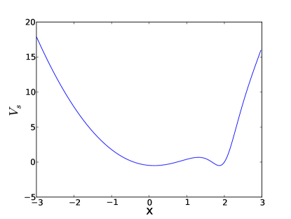
Figure 4: An asymmetric spring potential used to tether the chain. It has a second dip at approximately $x=2$

Plots are shown in Fig. 5 of $P_{1}(x)$ for four values of $x^{\prime}$ within a period.

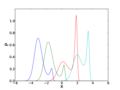
Figure 5: Plots of the probability distribution of $P_{1}$ as a function of position $x$ for different values of $x^{\prime}$ for the asymmetric spring model Eq. 21.

By integrating using these distributions, Eq. 14, the work can be obtained. With $c_{0}=0.025$ and $c_{1}=0.05$ the work $W_{L}=0.00080954$. With the $c_{i}$’s $10$ times those values, $c_{0}=0.25$, and $c_{1}=0.5$, $W_{L}=0.0025$.

Now we consider the case of a linear spring so that the nonlinear parameter $a=0$ in Eq. 21. Instead we make the periodic potential asymmetric by setting $A_{1}=A_{2}=2$ in Eq. 20, still with $c_{0}=0.25$, and $c_{1}=0.5$. Fig. 6 plots $P_{1}(x)$ for four values of $x^{\prime}$ within a period.

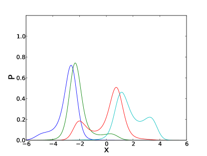
Figure 6: Plots of the probability distribution of $P_{1}$ as a function of position $x$ for different values of $x^{\prime}$ for an asymmetric periodic potential, but a linear spring.

In this case, the work $W_{L}=-0.1596$.

What the numerical results have shown is that asymmetry in the spring potential is quite ineffective at producing work, whereas asymmetry in the periodic binding potential is much more effective. We shall use this result below and concentrate on systems with symmetric spring potentials, but asymmetric potentials.

VII Unbound Equilibration Model

It is worthwhile to understand in more detail, what constrains the maximum force of photo-mechanical conversion by tuning the potentials employed and the binding rate. And to ask how the design will depend on the flux of photons. We are limited in our choice of the potentials $V_{0}$ and $V_{1}$ that both must be bounded. In this system, the unbound potential is not periodic which limits the amount of power that can be generated. In cases considered earlier ProstPRL , where both potentials are periodic, it is possible to get much more efficient motion by alternating between states with different potential maxima. However this is not relevant to our system.

To understand this better, it is useful to examine a limit where we can treat the system analytically. We therefore examining the case where the binding rate of unbound chain is sufficiently that we can regard it in thermal equilibrium.

The model is illustrated in Fig. 7. We take the unbound potential to be that of a linear spring below a cutoff

$$V_{s}=V_{0}=\begin{cases}kx^{2}/2,&\text{if $-l_{c}<x<l_{c}$}.\\ \infty,&\text{otherwise}.\end{cases}$$ (22)

we choose the spring coefficient $k$ and the cutoff length $l_{x}$ such that $l_{c}\exp(-kl_{c}^{2}/2)\ll 1$. Below, we will take $l_{c}=L/2$ or $\infty$.

The periodic potential $V_{p}$ is taken to be localized at periodic points (with a separation of $L$) that rapidly vary from a large maximum $V_{max}$ to a minimum $V_{min}$, as shown. We take the region over which this happens to be negligibly small compared to other length scales in the problem.

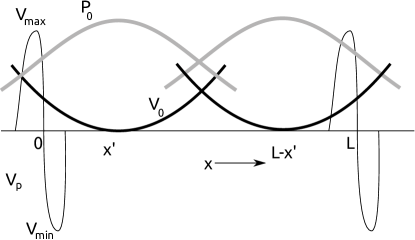
Figure 7: Illustration of the kind of potentials employed in the Unbound Equilibration Model. The periodic potential $V_{p}$ is nonzero only on small regions on the x-axis. It shows a large peak of height $V_{max}$ and large negative dip $V_{min}$. There spring potential $V_{0}$ is parabolic, except that it has a cutoff where it becomes infinite when stretched by more than $l_{c}$. The corresponding probability distribution $P_{0}$ (grey curve) is assumed to have relaxed to equilibrium. The spring potential is shown at two different position, when it is centered at $x^{\prime}$ and $L-x^{\prime}$.

To understand how equilibration can occur in this model, we can rewrite Eqs. 4 in the steady state limit

$$\nabla\cdot(\nabla-{\bf f}_{0})P_{0}({\bf r})-c_{0}P_{0}({\bf r})=-c_{1}P_{1}({\bf r})$$ (23a)

$$\nabla\cdot(\nabla-{\bf f}_{1})P_{1}({\bf r})-c_{1}P_{1}({\bf r})=-c_{0}P_{0}({\bf r})$$ (23b)

Although this is time independent, we consider the related time dependent equations for variables $\tilde{P}_{i}({\bf r},t)$

$$\partial_{t}\tilde{P}_{0}({\bf r})-\nabla\cdot(\nabla-{\bf f}_{0})\tilde{P}_{0}({\bf r})=0$$ (24a)

$$\partial_{t}\tilde{P}_{1}({\bf r})-\nabla\cdot(\nabla-{\bf f}_{1})\tilde{P}_{1}({\bf r})=0$$ (24b)

where $P_{i}$, $i=0,1$, is the Laplace transform of $\tilde{P}_{i}$, $P_{i}(s)={\cal L}\{\tilde{P}_{i}\}$, where the conjugate variable for equations (a) and (b) are $s=c_{0}$ and $s=c_{1}$, respectively. The initial conditions on each equation are

$$\tilde{P}_{0}({\bf r},t=0)=c_{1}P_{1}({\bf r},s=c_{1})$$ (25a)

$$\tilde{P}_{1}({\bf r},t=0)=c_{0}P_{0}({\bf r},s=c_{0})$$ (25b)

These equation have a direct physical interpretation. The left hand sides in Eqs. 24 are those of particles in diffusing in potentials but with conservation of particles. For long enough times, independent of initial conditions, the solution to these equations will go to thermal equilibrium given by the Gibbs distribution. Eq. 24a describes diffusion in a quadratic potential. We require that we are probing this at long enough times $t$, so that it will have nearly reached this equilibrium state. Call this longest relaxation time $\tau_{0}$. The solution to the diffusion equation $\tilde{P}({\bf r},t)$ for either of Eqs. 24, can be written as a sum over spatial eigenfunctions, $\phi_{n}({\bf r})$ that decay at different rates $\lambda_{n}$, (arranged to be monotonically increasing):

$$\tilde{P}({\bf r},t)=\sum_{n=0}^{\infty}\phi_{n}({\bf r})\exp(-\lambda_{n}t),$$ (26)

of which the smallest $\lambda$, $\lambda_{0}=0$, corresponds to the equilibrium state. The relaxation time is $\tau_{0}=1/\lambda_{1}$, Thus the Laplace transformed variable $P$ can be written

$$P({\bf r},s)=\sum_{n=0}^{\infty}\phi_{n}({\bf r})\frac{1}{s+\lambda_{n}}.$$ (27)

If the $n=0$ term is to dominate, we therefore require $s=c_{0}\ll 1/\tau_{0}$. The physical interpretation of this condition is that binding typically occurs only after many relaxation times of the unbound end.

$P_{0}({\bf r},s=c_{0})$ will be dominated by the first term in Eq. 27 and therefore proportional to the eigenfunction $\phi_{0}({\bf r})$ which is the equilibrium distribution and is $\propto\exp(-V_{0})$. An important simplifying point in the above approach is that the precise form of the initial condition Eq. 25a is not not important, but because of particle conservation, only the total area under $P_{1}$ affects the result.

Now we consider the solution for $P_{1}$. If we consider unbinding times much longer than the relaxation time in the bound state, we also arrive a thermal equilibrium, which as was shown by Eq. 17 to lead to no work being performed. Instead we will consider situations where there are very long lived metastable states. In Fig. 7, the potential seen by a particle in Eq. 24b is $V_{1}=V_{0}+V_{p}$. If a particle starts between $0$ and $L$, it will remain trapped in that region for a Kramer’s time which (ignoring algebraic pre-factors) depends on $x^{\prime}$, but has a minimum value of $\tau_{m}\propto\exp(V_{max})$. By choosing large enough $V_{max}$ this can be made arbitrarily long.

A particle in such a metastable state will relax to a metastable equilibrium, obeying Eq. 26 that will eventually fail for times $t>\tau_{m}$. In this expansion, the longest relaxation time to this metastable state $\tau_{1}=1/\lambda_{1}$, will be taken to be much smaller than $\tau_{m}$. Thus the above argument on the range of $c_{0}$ can be used mutatis mutandis to restrict the unbinding rate to $1/\tau_{m}\ll c_{1}\ll 1/\tau_{1}.$

In this regime we can understand the solution to Eqs. 24b and 25b by considering the corresponding Greens function $\tilde{G}({\bf r},t;{\bf r}_{0})$. We replace the initial condition Eq. 25b by

$$\tilde{G}_{1}({\bf r},t=0;{\bf r}_{0})=\delta({\bf r}-{\bf r}_{0}).$$ (28)

We can then obtain $\tilde{P}_{1}$ from the Greens function from

$$\tilde{P}_{1}({\bf r},t)=\int\tilde{G}_{1}({\bf r},t;{\bf r}_{0})c_{0}P_{0}({\bf r}_{0},s=c_{0})d^{d}{\bf r}_{0}.$$ (29)

For a wide range of times, and regions of ${\bf r}^{\prime}$, the $\tilde{G}_{1}$ will approach the same metastable state. A particle starting at any point within a certain region will end up stuck in the same state and hence approach the same metastable equilibrium. Confining our attention to the one dimension model of Fig. 7, for $0<x_{0}<L/2$ the solution will be strongly localized at the minimum $x=0$. For $L/2<x_{0}<L$ the effects of $V_{p}$ are negligible and $\tilde{P}_{1}(x)\propto\exp(-V_{0})$. This is because the potential $V_{0}$ in Eq. 22 is cutoff which does not allow the particle to visit the $x=0$ region. Hence the effect of $V_{p}$ is only seen close to $x=L$ where it provides a strong repulsion, but over a negligibly small region of $x$. For $-L/2<x_{0}<0$, $V_{p}$ also does not contribute. For $L<x_{0}<3L/2$ the solution will be strongly localized at the minimum at $x=L$. Because of particle conservation, the area under $\tilde{G}_{1}$ is always unity.

A physical interpretation of the above equations in terms of a one dimensional one particle system can now be made using the Laplace transformed variables and the metastable limit considered above is now apparent. In the unbound state, the particle reaches thermal equilibrium relaxing to the Gibbs distribution, $P_{0}\propto\exp(-V_{0})$. Then the periodic potential $V_{p}$ is suddenly added in. The position at the time of switching is labeled $x_{0}$. Depending on which interval $x_{0}$ is in, $x$ will equilibrate to the corresponding metastable equilibrium with $P_{1}\propto\exp(-V_{1})$ and is completely confined to that interval. The relative probabilities being in one of the three above regions is obtained by the area under $P_{0}$ for that interval.

Now we know how to determine $P_{0}$ and $P_{1}$, we would like to calculate the work $W_{L}$ given by Eq. V. Because of the symmetric form assumed for $f_{s}$, the $f_{0}P_{0}$ term in the integrand gives zero contribution and we are left with

$$W_{l}=\int_{0}^{L}\int_{-\infty}^{\infty}f_{0}(x-x^{\prime})P_{1}(x,x^{\prime})dxdx^{\prime}$$ (30)

and consider first how to calculate the inner integral

$$f_{l}(x^{\prime})\equiv\int_{-\infty}^{\infty}f_{0}(x-x^{\prime})P_{1}(x,x^{\prime})dx$$ (31)

where $x^{\prime}$ is the position of the tethered end. Eq. 22 gives $f_{0}(x)=-kx$ for $|x|<L/2$.

Using the prescription we have found for $P_{1}(x,x^{\prime})$, which is simplified by the above physical interpretation, we can partition this integral into the different $x$-intervals of metastability: $I_{-}\equiv[-L/2,0]$, $I_{0}\equiv[0,L]$, and $I_{+}\equiv[L,3L/2]$. The value of $P_{1}(x,x^{\prime})$ depends on the probability of initially being trapped in one of those three intervals. Because of the cutoff we have imposed on $V_{0}$, only two intervals need be considered for a given value of $x^{\prime}$. For $0<x^{\prime}<L/2$, only intervals $I_{-}$ and $I_{0}$ occur. The probability that $x\in I_{-}$ given $x^{\prime}$ is

$$E(x^{\prime})\equiv Prob(x\in I_{-}|x^{\prime})=\int_{-\infty}^{0}p_{0}(x-x^{\prime})dx=\int_{x^{\prime}}^{\infty}p_{0}(x)dx$$ (32)

and the probability that $x\in I_{0}$ that is, $P(x\in I_{0}|x^{\prime})=1-E(x^{\prime})$. Here $p_{0}(x)$ is proportional to $P_{0}(x)$ but normalized to unity, to simplify the presentation. We can obtain the values for $L/2<x^{\prime}<L$ by symmetry, so that $P(x\in I_{+}|x^{\prime})=E(L-x^{\prime})$ and $P(x\in I_{0}|x^{\prime})=1-E(L-x^{\prime})$. $E(x)$ is simply related to the complementary error function in the limit considered here, where the effects of the cutoff in the potential will have negligible effect, $E(x)=\frac{1}{2}erfc(\sqrt{k}x)$.

There is a symmetry in many of the quantities considered, as shown in Fig. 7 where the potential $V_{0}$ and corresponding probability distribution $p_{0}$ is for the tethering point at $x^{\prime}$ and at $L-x^{\prime}$. Therefore it is convenient to consider $f_{l}(x^{\prime})+f_{l}(L-x^{\prime})$. This can be written as

$$-\frac{kc_{0}}{c_{0}+c_{1}}(- E (x^{\prime})\langle x\rangle^{\prime}+E(x^{\prime})x^{\prime}$$

$$-( 1 -E(x^{\prime}))x^{\prime}+(1-E(x^{\prime}))\langle x\rangle^{\prime\prime})$$ (33)

where

$$\langle x\rangle^{\prime}\equiv-\frac{\int_{-\infty}^{0}(x-x^{\prime})p_{0}(x-x^{\prime})dx}{\int_{-\infty}^{0}p_{0}(x-x^{\prime})dx}=\frac{\int_{x^{\prime}}^{\infty}xp_{0}(x)dx}{E(x^{\prime})}$$ (34)

and

$$\langle x\rangle^{\prime\prime}\equiv-\frac{\int_{-\infty}^{0}(x+x^{\prime})p_{0}(x+x^{\prime})dx}{\int_{-\infty}^{0}p_{0}(x+x^{\prime})dx}=\frac{-E(x^{\prime})}{1-E(x^{\prime})}\langle x\rangle^{\prime}.$$ (35)

The four terms in Eq. VII correspond to contributions from respectively regions $I_{-}$, $I_{+}$ , $I_{0}$, and $I_{0}$. The first and third term are contributions from $f_{l}(x^{\prime})$ and the others are from $f_{l}(L-x^{\prime})$. The factors involving $c$ give the correct normalization according to Eq. 12. Combining the above equations,

$$W_{L}=\frac{2kc_{0}}{c_{0}+c_{1}}\int_{0}^{L/2}2E(x^{\prime})(\langle x\rangle^{\prime}-x^{\prime})+x^{\prime}dx^{\prime}.$$ (36)

In the limit of large $L$, which we are considering by virtue of the condition on the cutoff in $V_{0}$ imposed by Eq. 22, the integrand simplifies because $\langle x\rangle^{\prime}$ becomes exponentially close to $x^{\prime}$, and the only term remaining is $x^{\prime}$. Thus for large $L$, $W_{L}=(c_{0}/(c_{0}+c_{1}))kL^{2}/4$ The factors involving the $c$’s represent the fraction of time spent in the bound configuration. The last term increases quadratically with $L$. This result is misleading if not taken with the appropriate limits that have been assumed in its derivation. The factor $(c_{0}/(c_{0}+c_{1}))$ is very close to unity as we are assuming that the relaxation time in the unbound state is much faster than in the bound state, hence $c_{0}\gg c_{1}$. However the work $W_{L}$ to move a distance $L$ was assumed to be in the adiabatic limit, and here the time scales associated with bound state relaxation are exponentially long. This is because to reach this metastable equilibrium the particle has to hop over barriers of size $V_{0}(x^{\prime})$, see Fig. 7. Hence the longest relaxation time for this is at $x^{\prime}=L/2$ and is of order $\exp(kL^{2}/4)$. Note that this does not contradict our assumption that we are still in a region of metastability, which requires times much less than $\exp(V_{max})$. But for this to work, we require that $V_{max}\gg V_{0}(L/2)$

Now we consider the case where the spring length cutoff $l_{c}\rightarrow\infty$. The disadvantage of this is that the chain end can, in principle, hop over many barriers ending up arbitrarily far from the tether point, and that these hopping times should be included in the above analysis. However, the probability of such a hop becomes negligible when the probability of finding the chain end there is small. Hence we still have a clear separation of time scales between metastable states as discussed above, and fully equilibrated system, which requires surmounting the energy barrier $V_{max}$. In this case, we can therefore assume that when the chain end $x^{\prime}$ is between $nL$ and $(n+1)L$, it will strongly localized at $x^{\prime}=nL$. Therefore

$$f_{l}(x^{\prime})=-k\sum_{n=-\infty}^{\infty}\Delta_{n}(x^{\prime})(nL-x^{\prime})$$ (37)

where $\Delta_{n}(x^{\prime})$ is the probability of initially finding the chain end between $nL$ and $(n+1)L$,

$$\Delta_{n}(x)=E(nL-x)-E((n+1)L-x).$$ (38)

It is easily seen that $\Delta_{-n}(L-x)=\Delta_{n}(x)$. Using this and Eq. 37

$$f_{l}(L-x)=-k(-f_{l}(x)-L\sum_{n=-\infty}^{\infty}\Delta_{n}(x^{\prime}))=-f_{l}(x)+kL.$$ (39)

To obtain the work, we follow the same procedure as above and consider $f_{l}(x^{\prime})+f_{l}(L-x^{\prime})$, which here is just $kL$. Therefore in this case,

$$W_{L}=\frac{c_{0}}{c_{0}+c_{1}}\frac{kL^{2}}{2}$$ (40)

which in this model exactly, for all $k$ and $L$, given that we are in a region of strong metastability.

VII.1 Efficiency in large power stroke limit

We now are in a position to answer a central question about the performance of this kind of device: is the efficiency limited by the small value of $k_{B}T$ compared to photon energies? We have seen from the above analysis that it is possible to get arbitrarily large forces developing at the expense of exponentially slow operation. However this is in the limit of infinitesimal plate velocity $\rm v$. In contrast, the power obtained is instead average force times this, $\langle f\rangle{\rm v}$ and we would like to operate the device at the velocity of maximum power, which necessitates the operation of it far from equilibrium, because compensating the increase in $\rm v$ is a decrease in $\langle f\rangle$ due to dissipation. It could be that the optimum velocity of operation decreases very quickly with $kL^{2}/2$ meaning that the device becomes increasingly inefficient as the spring constant $k$ is increased. This would make it impossible to harvest more than of order $k_{B}T$ energy per cycle.

The efficiency is defined as the ratio of the amount of power produced to the amount of power put in. The amount of energy needed to dissociate a polymer end from a binding site is $V_{min}$. Binding to $V_{min}$ must produce an energy less than that of an unbound polymer. The power put in is $V_{min}c$ where $1/c=1/c_{0}+1/c_{1}$. Therefore the efficiency is

$$\eta=\frac{\langle f\rangle{\rm v}}{cV_{min}}.$$ (41)

To investigate this problem further, the one dimensional model of the last section with $l_{c}\rightarrow\infty$ was implemented using Metropolis Monte Carlo. We chose the periodic potential $V_{p}$ to vary as

$$V_{p}(x)=\begin{cases}-4V_{min}\frac{x}{\delta}(1-\frac{x}{\delta}),&\text{if $0<x<\delta$}.\\ -4V_{max}\frac{x}{\delta}(1+\frac{x}{\delta}),&\text{if $0>x>-\delta$}.\\ 0,&\text{otherwise}.\end{cases}$$ (42)

Here we set $\delta=0.1$, $V_{max}=V_{min}=100$, and $L=1$. In order to preserve diffusional dynamics, steps in x were attempted uniformly in the range $[-0.025,0.025]$ ensuring that the periodic potential cannot be jumped across in one move. One move increased the time by $.05$, though this number was arbitrary and aside from an obvious rescaling, does not affect the results obtained.

To observe behavior in the limit of metastability as discussed in the previous section, the rate of unbinding must be set to be small compared to the inverse metastable equilibration time in the bound state. Hence we chose the unbinding rate $c_{0}=10^{-5}$ and $c_{1}=5\times 10^{-4}$.

As the simulation was running, the tether point was moved at velocity $\rm v$ which was typically small, The average spring force $\langle f\rangle$ was measured as a function of $\rm v$ for a given spring constant $k$. The results of a run of $3\times 10^{10}$ steps are shown in Fig. 8(a).

(a)

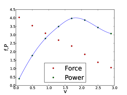
(b)

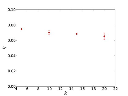
Figure 8: (a) The force and power versus velocity for the one dimensional model described in the text. Here the spring coefficient $k=15$. The line going through the power is a cubic spline fit used to more accurately determine the maximum value of the power. The velocity and power are both in units of $10^{-6}$. (b) A plot of the efficiency of the motor as a function of the spring constant $k$. Three separate runs, each of $3\times 10^{10}$ steps were used to determine the error bars, for each data point shown.

We are interested in the limit of large $k$ although this is hard to achieve numerically owing to exponentially long relaxation times. The parameters used allow us to probe up to $k=20$. In the large $k$ limit, the minimum value of $V_{min}$ needed to bind, is $kl^{2}/2$, where $l$ is the maximum amount the spring will need to stretch from the tether to the binding site. Because $\delta=0.1$ and $L=1$, this implies $l=0.9$. Therefore our formula for the efficiency, given this input energy is $\eta=P_{max}/(ckl^{2}/2)$, where $P_{max}$ is the maximum of the power versus velocity, as shown in Fig. 8(a). Plotting the efficiency for different values of $k$ ranging from $5$ to $20$ yields the points in Fig. 8(b). Despite the fact that the relaxation time for metastable relaxation of the system varies over more than two orders of magnitude, the overall efficiency is almost constant. We expect at higher value of $k$, the efficiency will eventually drop owing to the fact that the average unbinding time becoming smaller than the metastable relaxation time.

What the above analysis shows is that in the limit where the photon cross section can be made arbitrarily low, the efficiency can be adjusted to be constant, independent of the photon energy. This is accomplished by choosing a large spring coefficient. In reality with photon energy of $2eV$ and $k_{B}T\approx 1/40eV$, photon flux would have to be far too low for this optimal regime to be realizable. However the above analysis also shows that the efficiency can be substantially increased by choosing larger $k$ at the expense of lowering the cross section. The energy delivered in one cycle should scale as $E_{c}=kL^{2}$. This can be increased to be substantially larger than thermal energies but at the expense of a long relaxation time proportional to $\exp(E_{c}/k_{B}T)$. As noted earlier, it should be possible to make $E_{c}$ about $7k_{B}T$, with reasonable parameter estimates.

VIII Conclusions

Here we have analyzed the viability of converting photons to mechanical energy using a device composed of an canted polymer brush tethered to a lower plate but able to bind its other ends to sites on an upper plate. Photons can dissociate these ends from binding sites. By a combination of analytical and numerical arguments we showed that in steady state, this produces net mechanical power.

The system is inspired by biological motors such as myosin II that bind to actin and is dissociated by the binding of ATP. The analysis used here could also be applied to such systems, however in reality they contain many more stages. In general, these kind of systems are classified as “thermal ratchets" ReimannRev , where the system can be thought of as moving in a washboard potential in the presence of thermal noise. Though that description can be very useful in understanding the general principles behind the operation of such motors, in the present case, we are trying to model the system in more detail than such models can afford. Instead we have described the system using Langevin dynamics and also two coupled Fokker-Planck equations similar in spirit but not identical to previous approaches ProstPRL ; BustamanteKellerOster . The difference here is that for potentials to be a sensible model for a polymer tethered to a single point, they cannot be periodic. Such modelling allows us to see how varying microscopic parameters affect the power and force characteristics.

The analytical results on the Unbound Equilibration Model and extensive one dimensional simulations, show that the force applied by the device can be made arbitrarily large at the expense of having exponentially long relaxation times. At a given photon flux, the production of large forces from single polymers imply the need for a very low cross section of interaction between the photon and the bound end plus binding site, as long relaxation times are required. Therefore there is a trade off between this force and the speed the device can move. This may be circumvented to some extent by stacking transparent devices of this kind, so that even though the cross-section of interaction of an individual photon with a given layer is low, it will eventually be captured by one layer.

Therefore it appears that there is no theoretical obstacle to prevent the photo-mechanical conversion of energy in this manner, however it represents a significant experimental challenge.

It has been pointed out GrzybowskiReview that there is an important distinction between artificial molecular switches and artificial molecular machines, the former being a fraction of a penny, and the latter being extremely challenging to create. The approach investigated here is closer to biological motors than other proposals, and should be more forgiving about randomness, either during fabrication, or due to thermal motion, than approaches that require precise chemical synthesis of molecules capable of sophisticated conformational changes credi2006 . However its experimental realization is still quite clearly a formidable task.

IX Acknowledgments

The author would like to thank Professor Monica Olvera de la Cruz and Edward Santos for useful discussions. Support from National Science Foundation CCLI Grant DUE-0942207 is gratefully acknowledged.

References

- (1) M. Irie and D. Kunwatchakun, Macromolecules, 19 (10), pp 2476-2480 (1986).
- (2) M. Irie, Advances in Polymer Science, , 94, 27-67 (1990).
- (3) M. Suzuki and O. Hirasa, Adv Poly Sci 110 241 (1993).
- (4) M. Behl and A. Lendlein, Soft Matter, 3, 58-67 (2007)
- (5) I. Roy and M. N. Gupta, 10 1161–1171 (2003).
- (6) A. Credi, Aust. J. Chem. 59, 157 (2006).
- (7) M. K. J. ter Wiel, R. A. van Delden, A. Meetsma, B. L. Feringa, J. Am. Chem. Soc. 127, 14208 (2005).
- (8) N. Ruangsupapichat, M. M. Pollard, S. R. Harutyunyan and B. L. Feringa, Nature Chem. 3 53 (2011).
- (9) J. Vicario, M. Walko, A. Meetsma, and B. L. Feringa, J. Am. Chem. Soc. 128, 5127 (2006).
- (10) P. R. Ashton, R. Ballardini, V. Balzani, E. C. Constable, A. Credi, O. Kocian, S. J. Langford, J. A. Preece, L. Prodi, E. R. Schofield, N. Spencer, J. F. Stoddart and S. Wenger, Chem. Eur. J. 4, 2413 (1998).
- (11) P. R. Ashton, R. Ballardini, V. Balzani, A. Credi, R. Dress, E. Ishow, C. J. Kleverlaan, O. Kocian, J. A. Preece, N. Spencer and J. F. Stoddart, M. Venturi, S. Wenger, Chem. Eur. J. 6, 3558 (2000).
- (12) J. Berná, D. A. Leigh, M. Lubomska, S. M. Mendoza, E. M. Pérez, P. Rudolf, G. Teobaldi, and F. Zerbetto, Nature Mat. 4, 704 (2005).
- (13) Y. Liu, A. H. Flood, P. A. Bonvallett, S. A. Vignon, B. H. Northrop, H.-R. Tseng, J. O. Jeppesen, T. J. Huang, B. Brough, M. Baller, S. Magonov, S. D. Solares, W. A. Goddard, C. M. Ho and J. F. Stoddart, J. Am. Chem. Soc. 127, 9745 (2005).
- (14) C. Bustamante, D. Keller, and G. Oster, Acc. Chem. Res. 34 412 (2001).
- (15) J. Prost, J.-F. Chauwin, L. Peliti, and A. Ajdari, Phys. Rev. Lett. 72 2652 (1994).
- (16) E. Klampaftis, D. Ross, K. R. McIntosh, and B. S. Richards, Solar Energy Materials and Solar Cells, 93, 1182−1194. (2009).
- (17) N.-P. Harder and P. Würfel, Semiconductor Science and Technology, 18 S151 (2003).
- (18) J.M. Deutsch Phys. Rev. E 81, 061804 (2010).
- (19) P. Reimann and P. Hänggi, Appl. Phys. A 75 169 (2002).
- (20) F. Jülicher, A. Ajdari, and J. Prost, Rev. Mod. Phys., 69, (1997).
- (21) W.H. Press, S.A. Teukolsky, W.T. Vetterling and B.P. Flannery "Section 18.1. The Shooting Method". Numerical Recipes: The Art of Scientific Computing (3rd ed.). New York: Cambridge University Press (2007).
- (22) A. Coskun, M. Banaszak, R. D. Astumian, J. F. Stoddart and B. A. Grzybowski, Chem. Soc. Rev., 41, 19 (2012).